High-Order, Finite-Volume Methods in Mapped Coordinates

More documents

Recommendations

Info

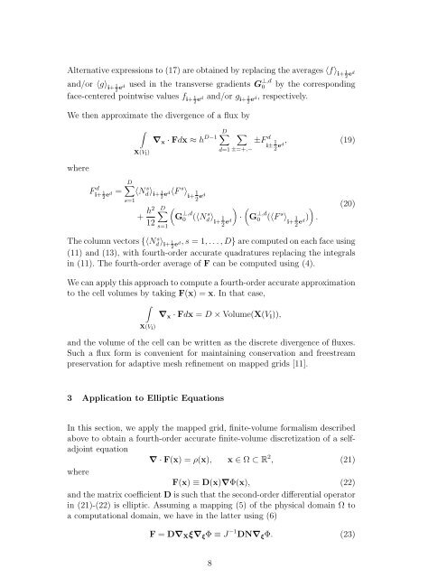
Alternative expressions to (17) are obtained by replacing the averages 〈f〉 i+12 edand/or 〈g〉 i+1 used in the transverse gradients G ⊥,d2 ed 0 by the correspondingface-centered pointwise values f i+1 and/or g 2 ed i+ 1 ed, respectively.2We then approximate the divergence of a flux bywhere∫X(V i )∇ x · Fdx ≈ h D−1D ∑∑d=1 ±=+,−±F di± 1 (19)ed,2F di+ 1 2 ed =D∑〈Nd〉 s i+1ed〈F s 〉 12 i+s=1+ h2 D∑12s=12 ed()G ⊥,d0 (〈Nd〉 s 1 i+·2 ed()G ⊥,d0 (〈F s 〉 1 i+ ed) .2(20)The column vectors {〈Nd〉 s i+1ed, s = 1, . . . , D} are computed on each face using2(11) and (13), with fourth-order accurate quadratures replacing the integralsin (11). The fourth-order average of F can be computed using (4).We can apply this approach to compute a fourth-order accurate approximationto the cell volumes by taking F(x) = x. In that case,∫∇ x · Fdx = D × Volume(X(V i )),X(V i )and the volume of the cell can be written as the discrete divergence of fluxes.Such a flux form is convenient for maintaining conservation and freestreampreservation for adaptive mesh refinement on mapped grids [11].3 Application to Elliptic EquationsIn this section, we apply the mapped grid, finite-volume formalism describedabove to obtain a fourth-order accurate finite-volume discretization of a selfadjointequation∇ · F(x) = ρ(x), x ∈ Ω ⊂ R 2 , (21)whereF(x) ≡ D(x)∇Φ(x), (22)and the matrix coefficient D is such that the second-order differential operatorin (21)-(22) is elliptic. Assuming a mapping (5) of the physical domain Ω toa computational domain, we have in the latter using (6)F = D∇ X ξ∇ ξ Φ ≡ J −1 DN∇ ξ Φ. (23)8
Following (19) and (20), we therefore obtain∫X(V i )∇ x · Fdx = h 23∑∑d=1 ±=+,−±F di± 1 2 ed + O ( h 4) , (24)where, using face-centered pointwise values of F in the transverse gradients,〈〉3∑F di+ 1 ≡ 〈F d〉 1 = ∂Φ2 ed i+˜D dd ′2 ed ∂ξd ′ =1d ′i+ 1 ⎡2 ed3∑=〈˜D 〈〉⎣ ∂Φdd ′〉i+ 1 d ′ =12 ed ∂ξ d ′i+ 1 2 ed+ h212 G⊥,d 0(〈˜D dd ′〉)i+ 1 · G⊥,d 0ed2( ∂Φ∂ξ d ′)i+ 1 2 ed ⎤⎦(25)where˜D ≡ (˜D dd ′)≡ J −1 N T DN. (26)Face averages 〈˜D dd ′〉can be computed to fourth order in terms of face averagesof the entries of the factor matrices N T , D and J −1 N using the productformula (17). Computing the second-order accurate transverse gradientsG ⊥,d0(〈˜D dd ′〉)i+ 1 ≡ 1 (〉〈˜D dd ′2 ed hi+ 1 − 〈˜D )〉dd2 ed +e d′ ′i+ 1 , (27)2 ed −e d′it then remains to specify the discretization of the averages 〈∂Φ/∂ξ d ′〉 1 i+2 edand transverse gradient G ⊥,d0 (∂Φ/∂ξ d ′) 1 i+ ed. 23.1 Discretization of 〈∂Φ/∂ξ d ′〉 1 i+and G⊥,d 0 (∂Φ/∂ξed d ′) 1 i+2 2 edFirst consider the case where d ′ = d. We have〈 ∂Φ∂ξ d〉i+ 1 2 ed =( )∂Φ+ h2 ∂Φ∆⊥,d + O ( h 4) , (28)∂ξ d 24 ∂ξ d i+ 1 2 edwhere ∆ ⊥,d is the Laplacian in the directions transverse to the d-th direction.Definingβ i+12 ed ≡ 1 24 [27 (Φ i+e d − Φ i) − (Φ i+2e d − Φ i−e d)] , (29)9
Page 1 and 2: High-Order, Finite-Volume Methods i
Page 3 and 4: the exact enforcement of the metric
Page 5: If we define control volumes in phy
Page 10: β 1 i+2 ed +e❞ ❞ ❞ d′❞β
Page 13 and 14: ✠Dirichlet boundaryDCBAFig. 3. Lo
Page 15 and 16: 10.80.60.40.20−0.2−0.4−0.6−
Page 17: 10 −2 N10 −310 −410 −510
Page 21 and 22: 3Runge Kutta Stability Domain21Im z
Page 23 and 24: Magnitude of Amplification FactorRe
Page 26 and 27: L ∞ Error Norm for Base SchemeN c
Page 28 and 29: 10 0 Uniform Advection of Sinusoida
Page 30 and 31: Note that, in computational space,
Page 32 and 33: 10 0 Uniform Advection of Compact D
Page 34 and 35: and/or face-centered values. Among

High-Order, Finite-Volume Methods in Mapped Coordinates

You also want an ePaper? Increase the reach of your titles

Delete template?

Save as template?