Chapter 5 Geodynamics - MIT

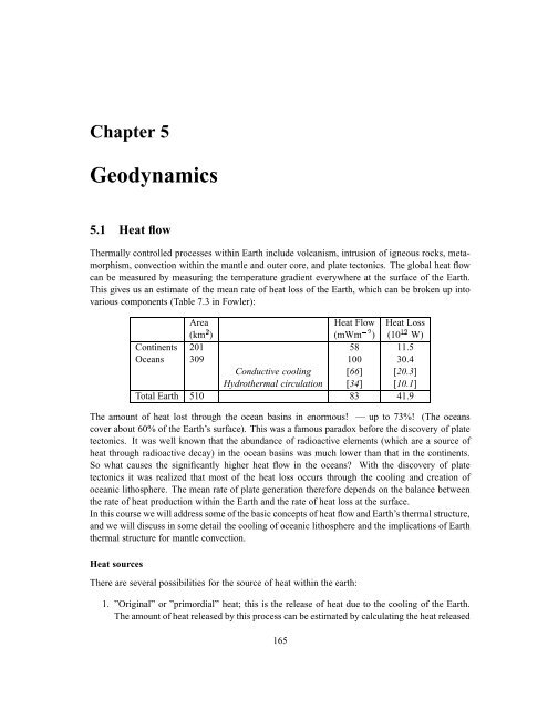
¦©¦©¨:172 CHAPTER 5. GEODYNAMICSFigure 5.5: Bathymetry changes with depth.convection; can the cooling oceanic lithosphere be considered as the Thermal Boundary Layer(across which heat transfer occurs primarily by conduction) of a large scale convection cell or issmall scale convection required to explain some of the observations discussed below? See therecent Nature paper by Stein and Stein, Nature 359, 123–129, 1992.Cooling of oceanic lithosphere: the half-space modelThe variation of temperature with time and depth can be obtained from solving the instant coolingproblem: material at a certain ¤temperature (or in Turcotte and Schubert) is instantly broughtto the surface temperature where it is exposed to surface temperature (see cartoons below; fora full derivation, see Turcotte and Schubert).Figure 5.6: The heating of a halfspaceDiffusion, or relaxation to some reference state, is described by error functions 2 , and the solutionto the 1D diffusion equation (that satisfies the appropriate boundary conditions) is given by ¤ 9 £¥¤§¦(5.11)© .£ ¢¡£ or §© ¦£©2 So called because they are integrations of the standard normal distribution.

¦£¥¤ ¦©¤£¦¨:¦:4¡5.3. THERMAL STRUCTURE OF THE OCEANIC LITHOSPHERE 173 ¤%9 £¥¤§¦(5.12)© .£ 9

:174 CHAPTER 5. GEODYNAMICSFigure 5.8: Cratonic and oceanic geotherms.Figure 5.9: Oceanic geotherms.as defined by (2) are hyperbola. From this, one can readily see that if the thermal lithosphere isbounded by isotherms, the £ thickness of the lithosphere increases as . For back-of-the-envelope© ¦¦ ¦¥©calculations you can use for lithospheric thickness. (For mm £ and : £Ma, which is the average age of all ocean oceanic lithosphere currently at ¢¡ ¦ ¦P ¤£ ¢¡ /the Earth’s surface,km). This thickening occurs because the cool lithosphere reduces the temperature of theunderlying material which can then become part of the plate. On the diagram the open circles depictestimates of lithospheric thickness from surface wave dispersion data. Note that even thoughthe plate is moving and the resultant geometry is two dimensional the half space cooling modelworks for an observer that is moving along with the plate. Beneath this moving reference pointthe plate is getting thicker and thicker.

¦99:¡£¦¡¡ ¡9©¡ ¡¡ ¡¡ ¡¡¦9:£¡¡ ¡£¥¤§¦©5.3. THERMAL STRUCTURE OF THE OCEANIC LITHOSPHERE 175Intermezzo 5.1 LITHOSPHERIC THICKNESS FROM SURFACE WAVE DISPERSIONIn the seismology classes we have discussed how dispersion curves can be used to extract informationabout lithospheric structure from the seismic data. The thickness of the high wave speed ’lid’, the structureabove the mantle low velocity zone, as determined from surface wave dispersion across parts of oceaniclithosphere of different age appears to plot roughly between the 900 and 1100 C isotherms,¡£¢£¤¦¥ §©¨¤¦¥ ¡or at about(see Figure 5.10). So the seismic ”lithosphere” seems to correspond to thermal lithosphere.In other words; in short time scales — i.e. the time scale appropriate for seismic wave transmission(sec - min) — most of the thermal lithosphere may act as an elastic medium, whereas on the longer timescale the stress can be relaxed by steady state creep, in particular in the bottom half of the plate. However,a word of caution is in order since this interpretation of the dispersion data has been disputed. Andersonand co-workers argue (see, for instance, Anderson & Regan, GRL, vol. 10, pp. 183-186, 1983) that interpretationof surface wave dispersion assuming isotropic media results in a significant overestimation of thelid thickness. They have investigated the effects of seismic anisotropy and claim that the fast¤isotropic¨¤¤LIDextends to a much cooler isotherm, at C, than the base of the thermal lithosphere.¡Figure 5.10: Elastic thickness.Heat flowIf we know the temperature at the surface we can deduce the heat flow by calculating the temperaturegradient:¡ ¡¡ ¦¡ (5.14)¡©© ¦© ¦ ¤ 9 £¥¤§¦©¡ ¤9 with

¡¡ ¡£¥¤§¦©For the heat flow proper we take¦O¢¢¡ ¦¡ ¡(99¡©¡¡ ¡¤¤£££¥¡( is measured at the surface!) so that ¡¡©£££©£¥¢¡£¢¢176 CHAPTER 5. GEODYNAMICS¡¨§© §¡:¢ ©¦¥© (5.15): ¦¢ ©: ¦¢ ©¡¨§© § ¥so that© (5.16)9 ¦ ¤© ¢ ¦and¦;(5.17) ¦ ¤9 ¡© ¢ ¦with the conductivity (do not confuse with , the diffusivity!). The important result is thataccording to the half-space cooling model the heat flow drops of as 1 over the square root of the¦age of the lithosphere. The heat flow can be measured, the lithospheric ¡age determined from, £ forinstance, magnetic anomalies, and if we assume values for the conductivity and diffusivity, Eq.(5.17) can be used to determine the temperature difference between the top and the bottom of theplate ¤ 9

5.4. THERMAL STRUCTURE OF THE OCEANIC LITHOSPHERE 177Figure 5.11: .Intermezzo 5.2 PLATE-COOLING MODELSThere are two basic models for the description of the cooling oceanic lithosphere, a cooling of a uniformhalf space and the cooling of a layer with some finite thickness. The former is referred to as the half-spacemodel (first described in this context by Turcotte and Oxburgh, 1967); The latter is also known as the platemodel (first described by McKenzie, 1967).Both models assume that the plate moves as a unit, that the surface of the lithosphere is at an isothermalcondition of 0 C, and that the main method of heat transfer is conduction (a good assumption, except at theridge crest). The major difference (apart from the mathematical description) is that in the half-space modelthe base of the lithosphere is defined by an isotherm (for instance 1300 C) so that plate thickness can growindefinitely whereas in the plate model the plate thickness is limited by some thickness .The two models give the same results for young plates near the ridge crest, i.e. the thickness is such that the”bottom” of the lithosphere is not yet ”sensed”. However, they differ significantly after 50 Myr for heat flowpredictions and 70 Myr for topography predictions. It was realized early on that at large distances from theridge (i.e., large ages of the lithosphere) the oceans were not as deep and heat flow not as low as expectedfrom the half-space cooling model (there does not seem to be much thermal difference between lithosphereof 80 and 160 Myr of age). The plate model was proposed to get a better fit to the data, but its conceptualdisadvantage is that it does not explain why the lithosphere has a maximum thickness of . The half spacemodel makes more sense physically and its mathematical description is more straightforward. Therefore,we will discuss only the half space cooling model, but we will also give some relevant comparisons withthe plate model.5.4 Thermal structure of the oceanic lithosphereBathymetryThe second thermal effect on the evolution of the cooling lithosphere is its subsidence or theincrease in ocean depth with increasing age. This happens because when the mantle materialcools and solidifies after melting at the MOR it is heavier than the density of the underlyingmantle. Since we have seen that the plate thickens with increasing distance from the MOR and ifthe plate is not allowed to subside this would result in the increase in hydrostatic pressure at somereference depth. In other words the plate would not be in hydrostatic equilibrium. But when the

¦© ¡§¤¢¦¦ ¡4 §¤¡¢4¤©©©¤¡¢¦4©178 CHAPTER 5. GEODYNAMICSlithosphere subsides, denser material will be replaced by lighter water so that the total weight of acertain column remains the same. The requirement of hydrostatic equilibrium gives us the lateralvariation in depth to the ocean floor. Application of the isostatic principle gives us the correctocean floor topography.Figure 5.12: Oceanic isostasy.¡ 224 4 ¤ (4¡ 2 . © /2(4 £ ¤ 4Let and represent the density of water kg/m ) and the mantle/asthenospherekg/m ), respectively, and the density as a function of time and depth withinthe cooling plate. The system is in hydrostatic equilibrium when the total hydrostatic pressure ofa column under the ridge crest at depth §£¢is the same as the pressure of a column of the samewidth at any distance from the MOR:¡£ (5.19)© .or4 ¤(5.20)¡ ©4 9

now use ¦¨with ¡ ©¦¦¦¦¦::¦¦©©©©©©¤¤¢©©¡¢¡¢9 §¦¤©¨©¤ 9 £¥¤§¦:¨£ ¦¤¦:¨¦:¨::5.4. THERMAL STRUCTURE OF THE OCEANIC LITHOSPHERE 179© .With £ , this gives (verify!!)¢¤¡¡ ©4 ¤ ¥4 9 4 ¤ ¤ 9 9© ¦£©¢¡ ¤9 © ¦4 ¤ ¥9£¥¤§¦£ ©¢¡£¥¤§¦£ ©(5.24)4 ¤ ¥ ¤9 © ¦£¢ ¤£ ¤ 4¥£©4 ¤we can change the integration boundary from to because at the base of the lithosphereand so that we can take the compensation a t any depth beneath the base of thecooling lithosphere (and erfc integrated from to is very small). If we also use ¡(see above) than we can write ¢¦ ©© ¦ ¢)£¥¤ ¦ ¡ ©4 ¤ ¥4 9

180 CHAPTER 5. GEODYNAMICScould cause anomalous topography (”thermal topography”) whereas the effect of deep dynamicprocesses in the Earth’s mantle can cause ”dynamic topography”. Removing the effects of conductionalone thus helps to isolate the structural signal due to other processes. This is likely tocontinue, perhaps with the new model (GHD1) by Stein & Stein (1992) instead of that by earlierworkers; since regional differences are often larger than the residual between observed and predictedheat flow and depth curves one could question how useful a (set of) simple model(s) is (are).For instance, if one allows the thermal expansion coefficient as a free parameters in the inversions,one might also look into allowing lateral variation of this coefficient. Davies and Richards arguethat the success of the cooling models in predicting the topography and heat flow over almost theentire age range of oceanic lithosphere (they attribute the deviations to the choice of the wrongsites for data — which is rather questionable) indicates that conductive cooling is the predominantmode of heat loss of most of the lithosphere (about 85% of the heat lost from the mantle flowsthrough oceanic lithosphere), which suggests that the lithosphere is the boundary layer of a convectivesystem with a typical scale length defined by the plates (plate-scale flow). They followup on a concept tossed up by Brad Hager that the oceanic lithosphere organizes the flow in thedeeper mantle. It is for arguments such as these that question as to whether or not the topographylevels off after, say, 80Ma, in not merely of interest to statisticians. It is quite clear that the detailsof the bathymetry of the oceans still contain significant keys to the understanding of dynamicprocesses in the deep interior of the Earth. One of the remarkable aspects of the square root oftime variation of ocean depth is that it does a very good job in describing the true bathymetry,even at distances pretty close to the MORs. This indicates that conduction alone is likely to bethe predominant mode of heat loss, even close to the MOR. The absence of any substantial dynamictopography near the ridge crest suggests that the active, convection related upwellings arenot significant. The upwelling is ”passive”: the plates are pulled apart (mainly as the result of thegravitational force, the slab pull, acting on the subducting slabs) and the asthenospheric mantlebeneath the ridges flows to shallower depth to fill the vacancy. In doing so the material will crossthe solidus, the temperature at which rock melts (which decreases with decreasing depth) so thatthe material melts. This process is known as decompression melting (see Turcotte & Schubert,Chapter 1), which results in a shallow magma chamber beneath the MOR instead of a very deepplume-like conduit.5.5 Bending, or flexure, of thin elastic plateIntroductionWe have seen that upon rifting away from the MOR the lithosphere thickens (the base ofthe/2thermallithosphere is defined by ¤ ,an isotherm, usually C) and subsides, and that the cooledlithosphere is more dense than the underlying mantle. In other words, it forms a gravitationallyunstable layer. Why does it stay atop the asthenosphere instead of sinking down to produce a morestable density stratification? That is because upon cooling the lithosphere also acquires strength.Its weight is supported by its strength; the lithosphere can sustain large stresses before it breaks.The initiation of subduction is therefore less trivial than one might think and our understanding ofthis process is still far from complete.The strength of the lithosphere has important implications:1. it means that the lithosphere can support loads, for instance by seamounts

2. define the constitutive relations between applied stress ¥ and resultant strain ¦5.5. BENDING, OR FLEXURE, OF THIN ELASTIC PLATE 181Figure 5.13: Pressure-release melting.2. the lithosphere, at least the top half of it, is seismogenic3. lithosphere does not simply sink into the mantle at trenches, but it bends or flexes, so that itinfluences the style of deformation along convergent plate boundaries.Investigation of the bending or flexure of the plate provides important information about the mechanicalproperties of the lithospheric plate. We will see that the nature of the bending is largelydependent on the flexural rigidity, which in turn depends on the elastic parameters of the lithosphereand on the elastic thickness of the plate.An important aspect of the derivations given below is that the thickness of the elastic lithospherecan often be determined from surprisingly simple observations and without knowledge of theactual load. In addition, we will see that if the bending of the lithosphere is relatively smallthe entire mechanical lithosphere behaves as an elastic plate; if the bending is large some of thedeformation takes place by means of ductile creep and the part of the lithosphere that behaveselastically is thinner than the mechanical lithosphere proper.5.5.1 Basic theoryTo derive the equations for the bending of a thin elastic plate we need to1. apply laws for equilibrium: sum of the forces is zero and the sum of all moments is zero:and ¤£¢¡P¦O¦;3. assume that the deflection ¨ , the typical length scale of the system, and 8 , the thicknessof the elastic plate ¡¨§ ¨ . The latter criterion (© 3) is to justify the use of linear elasticity.§

©¡£ ¦¦9¤ ¡©:©((¡©182 CHAPTER 5. GEODYNAMICSFigure 5.14: Deflection of a plate under a load.In a 2D situation, i.e., there is no change in the direction of , the bending of a homogeneous,elastic plate due to a ¢ load can be described by the fourth-order differential equation that iswell known in elastic beam theory in engineering:¡ ¢ ¢ (5.28) §¢¡ ¢¦ ¡ ©¢ with ¡ ¡the deflection, i.e., the vertical displacement of the plate, which is, in fact, theocean depth(!), the flexural rigidity, and a horizontal force.The flexural rigidity depends on elastic parameters of the plate as well as on the thickness of theplate:¦ ©¦ 8(5.29)with the Young’s modulus and the Poisson’s ratio, which depend on the elastic moduli and(See Fowler, Appendix 2).The bending of the plate results in bending (or fiber) stresses within the plate, ; dependingon how the plate is bent, one half of the plate will be in compression while the other half is inextension. In the center of the plate the stress goes to zero; this defines the neutral line or plane. Ifthe bending is not too large, the stress will increase linearly with increasing distance away fromthe neutral line and reaches a maximum at . The bending stress is also dependent on© £ 8the elastic properties of the plate and on how much the plate is ¥¥§¥ bent;curvature, with the curvature defined as the (negative of the) change in the slopeelastic moduli ¨ ¢ : ¡ ¢ ¡¨¢ (5.30)¥¥§¥ 8This stress is important to understand where the plate may break (seismicity!) with normal faultingabove and reverse faulting beneath the neutral line.The integrated effect of the bending stress is the bending moment , which results in the rotationof the plate, or a plate segment, in the £9 plane. ¢9£(5.31)¨¥¥§¥¨

¦¦¡¦5.5. BENDING, OR FLEXURE, OF THIN ELASTIC PLATE 183Figure 5.15: Curvature of an elastic plate.Equation (5.28) is generally applicable to problems involving the bending of a thin elastic plate.It plays a fundamental role in the study of such problems as the folding of geologic strata, thedevelopment of sedimentary basins, the post-glacial rebound, the proper modeling of isostasy, andin the understanding of seismicity. In class we will look at two important cases: (1) loading by seamounts, and (2) bending at the trench.Before we can do this we have to look a bit more carefully at the dynamics of the system. Ifwe apply bending theory to study lithospheric flexure we have to realize that if some loador moment causes a deflection of the plate there will be a hydrostatic restoring force owingto the replacement of heavy mantle material by lighter water or crustal rock. The magnitudeof the restoring force can easily be found by applying the isostasy principle and the effective£load is thus the applied load minus the restoring force (all per unit length in the direction):also makes clear that lithospheric flexure is in fact a compensation mechanism for isostasy! Foroceanic 544 ¤ 9 4¥¤ lithosphere . The bendingequation that we will consider is thus:E ¡ BC@CH£¢ 9$54¡6 with ¡ the deflection and 6 the gravitational acceleration. This formulation4 ¤ 9 4 and for continental flexure 54¡ ¢ ¢ (5.32) ¢ § ¡§ 54¡6¦ ©Loading by sea mountsLet’s assume a line load in the form of a chain of sea mounts, for example Hawaii.Figure 5.16: Deflection of an elastic plate under a line load.

¦¥ ¢ ¡¥§©¤£ ¢ ¢¡ ¥¥¥¦¨¡ ¢¡¥§¥¡ ¡ ¢¡¥¤£ ¢§¡ ¥¤£ ¢§¡ ¥184 CHAPTER 5. GEODYNAMICS¦ ¦ ¦ Let ¢ be ¢the load applied at and for . With this approximation we can¢¡ solve the homogeneous form of (5.32) for and take the©mirror image to get the deflection¢for . If we also ignore the ¡ horizontal applied force we have to ¢ solve ¢ ¡¡¦O(5.33)The general solution of (5.33) is ¢ § 54¡6©¢ ¡(5.34)¥ with the flexural parameter, which plays a central role in the extraction of structural informationfrom the observed data:¥¦(5.35)54?6 ©Figure 5.17: .The constants can be determined from the boundary conditions. In this case©9¦we can apply¦§ ¢¢ £the ¢ £general requirement that for so that, and we also require thatthe plate ¡ ¦Obe ¡ ¦; ¦O ¢horizontal ¢directly beneath : for so that : ¢the solution¦ ¡becomes¡ ©¦ ¡(5.36) ¢From this we can now begin to see the power of this method. The deflection as a function ofdistance is an oscillation with ¡¥ period and with an exponentially decaying amplitude. ¢©Thisindicates that we ¥ can determine directly from observed bathymetry ¢ profiles , and fromequations (5.36) and (5.29) we can determine the elastic ¡ thickness under the assumption of8

:¥¦(:¥(¥¡ ¢¡¥¥¡¢¥¤£ ¢§¡ ¥9¡9¢¦¢¢¦¥¢¦5.5. BENDING, OR FLEXURE, OF THIN ELASTIC PLATE 185values for the elastic parameters (Young’s modulus and Poisson’s ratio). The flexural parameter¥ has a dimension of distance, and defines, in fact, a typical length scale of the deflection (as afunction of the “strength” of the plate).Figure 5.18: A deflection profile.¦PThe constant can be determined from the deflection ¢ at and it can be shown (Turcotte © ¥&¡, the deflection beneath the center of the load. The final¡ Schubert) that ¡ ¦ © ¥expression for the deflection due to a line load is then¡ ©¦ ¥ ¡(5.37)Let’s now look at a few properties of the solution:¤The half-width of the depression can be found by solving for ¡ ¦;. From (5.37) it follows¢ ©¢ that . /..1 ¥¢ For¤£ ©¦;9¦¥ or ¢ ¢ ¢ the half-width of the depression is found ¥ to be ¢ ¢ ¡¥¤ ¤ ¤¦ ¡ ©¥ must be zero ¢ ¥ ¢¦¢¢¡,¡ ¢ ¤ ¦ ¢¥The height, , and location, , of forebulge find the optima of the solution (5.37). Bysolving we find that , and for those optima, For the location of the forebulge: and the¦§ . /..1 ¢ ©¦ .§£¢ , ¢© ¢ ¡§¦height of the forebulge ¡¨¤ ¦or ¡¥¤ ¦ / ¡ (very small!).Important implications: The flexural parameter can be determined from the location of either thezero crossing or the location of the forebulge. No need to know the magnitude of the load! Thedepression is narrow ¥ for small , which means either a weak plate or a small elastic thickness (orboth); for a plate with large elastic thickness, or with a large rigidity the depression is very wide.In the limit of very large the depression is infinitely wide but the amplitude , is zero nodepression at all! Once ¡ is known, information about the central load can be obtained from Eq. ¥(5.37)Note: the actual situation can be complicated by lateral variations 8 in thickness , fracturing of thelithosphere (which influences ), compositional layering within the elastic lithosphere, and by thefact that loads have a finite dimensions.9¡ Flexure at deep sea trenchWith increasing distance from the MOR, or with increasing time since formation at the MOR, theoceanic lithosphere becomes increasingly more dense and if the conditions are right 5 this gravi-5 Even for old oceanic lithosphere the stresses caused by the increasing negative buoyancy of the plate are not largeenough to break the plate and initiate subduction. The actual cause of subduction initiation is still not well understood,

£:¥¡¦¥£¡ ¡ ¢¡¥©¥: ¥ §£ £ ¢§¡ ¥ ¢¥¦99££:¤£ ¢¡ ¥186 CHAPTER 5. GEODYNAMICStational instability results in the subduction of the old oceanic plate. The gravitational instabilityis significant for lithospheric ages of about 70 Ma and more. We will consider here the situationafter subduction itself has been established; in general the plate will not just sink vertically intothe mantlebut it will bend into the trench region.Figure 5.19:£ £ ¡ ¦ ¦ ¢ ¢8 ©¢ £ ¦ ¦P ¢This bending is largely due to the gravitational force due to the negative buoyancy of the part ofthe slab that is already subducted . For our modeling we assume that the bending is due to anend load and a bending moment applied at the tip of the plate. As a result of the bendingmoment the slope at (note the difference with the seamount example wherethis slope was set to zero!). The important outcome is, again, that the parameter of our interest,the elastic thickness , can be determined from the shape of the plate, in vertical cross section,i.e. from the bathymetry profile !, in the subduction zone region, without having to know themagnitudes of and .We can use the same basic equation (5.33) and the general solution (5.34) (withforthe reason given above)©¢ ¡(5.38)¡ ¦ ¢9 9 but the boundary conditions are different and so are the constants and . At the bendingmoment 6 is and the end load . It can be shown (Turcotte & Schubert) that theexpressions for and are given byand ¥(5.39)¥ § so that the solution for bending due to an end load and an applied bending moment can be writtenas¡ ¦ ©¥ ¢¡(5.40)¡ ©¦ ¥¢ We proceed as above to find the locations of the first zero crossing and the fore bulge, or outerrise.but the presence of pre-existing zones of weakness (e.g. a fracture zone, thinned lithosphere due to magmatic activity —e.g. an island arc) or the initiation of bending by means of sediment loading have all been proposed (and investigated)as explanation for the triggering of subduction.6 At this moment, it is important that you go back to the original derivation of the plate equation in Turcotte &Schubert and realize they obtained their results with definite choices as to the signs of applied loads and moments —hence the negative signs.

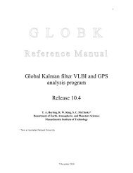
¥©¢¨¤9 ¢ ¢© ¥After a bit of algebra one can also eliminate ¥ to find the deflection ¡ ©:¥¦ £¢¡¤£9:¨9 ¢ ¢¤9 ¢ ©¢¡ ¢¦9¤£ 9£¨9 ¢ ¢¤9 ¢ © ¡ ¢¦5.5. BENDING, OR FLEXURE, OF THIN ELASTIC PLATE 187 £¡ ©¦O ©¦-¢ (5.41)¢ ¥ § ¥ ¡ ¢ © ¦O ¤ ¢In contrast to similar solutions for the sea mount loading case, these expressions ¢ for ¢ ¤andstill depend on and . In general and £ are unknown. They can, however, be eliminated,and we can show the dependence of £ ©¢ on ¢ and ¢ ¤, which can both be estimatedfrom the nathymetry profile. A perhaps less obvious but elegant way of doing this is to work out¡ © ¢ 9 ¢ ¤ . Using sine and cosine rules (see Turcotte & Schubert, 3.17) one finds that¥ 9 :¥ (5.42)(5.43)¦§so ¢¦ ¢ . .1". ¦O¦O ¦O /.©©¢that ¢, For one ¥ ¢ 9 ¢ ¤ ¢finds that , ¢ 9¤ § ¢ ¥ sothat the elastic thickness can be determined if one can measure 8 the horizontal distance betweenand¤ ¢ . ¢Figure 5.20: ©¢and . The normalized deflection¡¨¤as a function of normalized distance © ¢¤is known as the Universal Flexure Profile.¡9 ¢ ¢ ¤9 ¢ ¢ as a function of ¡ ¤ , ¢ ,¡ ©¦ ©¢¢(5.44)¢ ¡¥¤In other words, there is a unique way to bend a laterally homogeneous elastic plate so that it.'goesthrough the two ¢ points and ¢ ¤ . ¡¥¤ with the condition that the slope is zero at ¢ ¢ ¤.The example of the Mariana trench shown in Figure 5.20 demonstrates the excellent fit betweenthe observed bathymetry and the prediction after Eq. (5.44) (for a best fitting elastic thickness © © 8as determined from the flexural parameter calculated from equation (5.43).Bending stress and seismicityMany shallow earthquakes occur in near the convergent margin. Both in the overriding plates aswell as in the subducting plate. The latter can be attributed to the bending stresses in the plate. Thebending stress is given by Eq. (5.30). Earthquakes are most likely to occur in the region where the

4 © . Rewrite for ¤¤¡ 4 ¦©49¦¦¨¨¨4 ¡¡ © ¡4 ,¨©.4¢¨¡ §4 ¡¡ © ¡¤© ¦¨4 ¡ © ¡¦994¢¦¤¦44¡ 4 ¨¨5.6. THE UPPER MANTLE TRANSITION ZONE 189For a homogeneous medium (same composition and phase throughout) this equation simplifies to; (5.50)For the sake of the argument I will concentrate on the effect of adiabatic compression, i.e., thereis no variation of density with temperature.¡ (5.51)This assumption seems reasonable for most of the convecting mantle, and leads to the originalAdams-Williamson equation. For thermal boundary layers such as the lithosphere and the lowermostmantle (D”), and —- in case of layered convection — a TBL between the upper and thelower mantle, an additional gradient term has to be taken into account, and this modification hasbeen applied by Birch in his famous 1952 paper (see Fowler 4.3, and Stacey 5.3.1).For adiabatic self-compression the increase in pressure that results from the descent from radius§ to radius is due to the weight of the overlying shell with thickness ¡ , so that the pressuregradient can be written as:9*6?4with 6¦£¢¥¤©(5.52)The other term in Eq. (5.51), the pressure derivative of the density, can be evaluated in terms ofthe adiabatic bulk modulus ¦ £ :£¦ increase in pressure¦fractional change in volume ¡(5.53)Substitution of (5.52) and (5.53) in (5.51) and using (5.48) gives the Adams-Williamson equation:©¢ (5.54)4£ ¦which relates the density gradient to the known seismic parameter and the gravitational attractionof the ¤ mass©¤§¦©©¨¦¨£¤©©¨(5.55)the radius of EK F the Earth . The mass of the Earth is assumed to be know from astronomicaldata and is an important constraint on the density gradient. So the only unknown in (5.55) is the©©¨ density between EK F and . We can find a solution of (5.54) by working from the Earth’s4surface to larger depths: at the surface, the density of crustal rock is fairly well known so that thedensity gradient can be determined for the crust. This gradient is then used to estimate the densityat the base of the crust, which is then used to calculate the mass of the crustal shell. In this waywe can carry on the differentiation and integration to larger depths. As already mentioned, andexplicit in (5.55), any solution of (5.54) must agree with the total mass of the Earth, as well aswith the moment of inertia, which forms the second independent constraint on the solution. Thisprocess can only be applied in ¥regions where , and in this form one must also¨§EK F9¦ ¢ ¢shows that ¤© is, in fact, the mass of the Earth less the mass of the shell between point and¦¦O

¡¨¨¨¨192 CHAPTER 5. GEODYNAMICStransformation from £ Ol Sp will occur at a shallower depth than in the ambient mantle. Thismeans that for depths just less than 410 km the density within the slab is locally higher than inthe ambient mantle, and this, in fact, gives rise to an extra negative buoyancy force that helps theslab to subduct (it is an important plate driving force). At 660 km the dynamical effect of thephase change is the opposite. Inside and in the direct vicinity of the slab the phase boundary willbe depressed; consequently, the density in the slab is less than the density of the ambient mantlewhich creates a buoyancy force that will resist the further penetration of the slab.Figure 5.23: Effects of phase transformations on downgoingslabs.From the diagram it is clear that the steeper the Clapeyron slope, the stronger the dynamic effects.On the one hand, a lot of laboratory research is focused on estimating the slopes of these phaseboundaries in experimental conditions. On the other hand, and that brings us back to seismology,seismologists attempt to estimate the topography of the seismic discontinuity and thus constrainthe clapeyron slope and asses the dynamical implications. Important classes of seismological datathat have the potential to constrain both the sharpness of and the depth to the discontinuities arereflections and phase (mode) transformations. An example of a useful reflection is the underside¢¡¤¢¡£¡ ¡ ¡ ¡ reflection of ¡ ¡¦¥¨§ ¡ ¡¨¥¨§ the , or ¡ ¡ , or just ’, at the 660 km discontinuity.Since the ¡ paths of the ¡¨ =N= ¡phase and the are almost similar except for near the reflectionpoint, the difference in travel time gives direct information about the depth to the interface. Anotherexample is ©© the use © =N= © of underside reflections . Apart from proper phase identification(usually one applies stacking techniques to suppress signal to noise) the major problem with suchtechniques is that one has to make assumptions about upper mantle structure between the Earth’ssurface and the discontinuity, and these corrections are not always reliable. The time differencebetween the reflections at the surface and the discontinuity contains information about the depthto the interface, whereas the frequency content of both the direct and the reflected phase givesinformation about the sharpness of the interface. Also phase conversions can be used! This lineof research is still very active, and there is some consensus only about the very long wave lengthvariations in depth to the seismic discontinuities.

5.6. THE UPPER MANTLE TRANSITION ZONE 193Figure 5.24: The underside reflection off the 660 discontinuity.