A Turbomachinery Design Tool for Teaching Design Concepts for ...

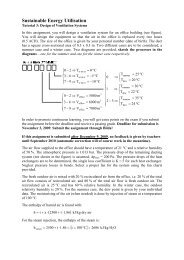
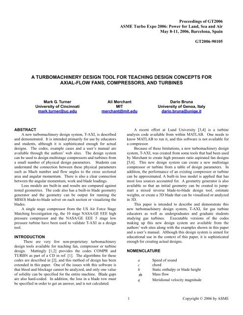
sACGreekαpRadiusEntropyAreaSpecific heat at constant pressureDR Diffusion ratioH Total enthalpyM Mach numberP PressureR Gas constantgasS Blade spacing, S = 2πr/ NbladesT TemperatureU Rotor wheel speedV Absolute velocityW Rotor relative velocityY Turbine loss coefficientZ Zweifel oefficientβδ*δγλθρσωωAbsolute flow angleRelative flow angleBlockage sourceBoundary layer displacement thicknessRatio of specific heatsBlockage coefficientTangential directionDensitySolidityRotor angular velocityCompressor loss coefficientSubscriptsh hubt tipx axialQ Heat TransferS Secondary flowT TotalW Workθ Tangential direction1 Leading edge2 Trailing edgeANALYSISFigure 1 is a schematic of the T-AXI TurbomachineryDesign System. It is made up of the T-AXI solver described indetail later in this section, as well as the compressor and turbinedesign modules and the turbine set-up module. The T-AXIsolver works with non-dimensional input. The “walls” filedefines the hub and casing geometry, and the “stack” fileincludes the details needed for each blade row including theleading and trailing edge geometry, the angular momentum atthe blade row trailing edge, the rotation speed, blockage, andnumber of airfoils.T-AXI is an axisymmetric solver. Most axisymmetricsolvers use a streamline curvature method as described bySmith [7] and Novak [8]. The method employed in the T-AXIsolver is more like the MISES algorithm [9,10]. Loss modelsare applied at each spanwise section depending on whether it isa compressor or turbine. To increase the robustness of thecalculation, the loss is smeared out just downstream of thetrailing edge. This has the effect of spanwise mixing describedby Adkins and Smith [11] with an extremely simple approach.The input “walls” and “stack” files can be created by handfor a general calculation. Detailed knowledge of the code nondimensionalizationand formatting are needed to do this.Alternatively, the compressor design code T-C_DES, theturbine design code T-T_DES, or the turbine set-up code T-2-T-AXI, can be used to automate the calculations based on designparameters. Straight leading and trailing edges are usedwithout contouring as well as a free-vortex assumption. Afourth approach to creating the input files for T-AXI is toextract the axisymmetric geometry, trailing edge angularmomentum and rotation rates from a 3D simulation. Thisapproach has been used for the SMI example case, but is toospecific to make available for general use.The input to T-C_DES is an “init” file, a “stage” file, andan optional “igv” file. If the “igv” file does not exist, it isassumed that there is no igv in the design. These files providetabular input to the code that is similar to COMPR developedby Mattingly [1]. The clearance ratio is the clearance dividedby radius. This is the tip radius for a rotor and hub radius for astator. For a preliminary compressor layout, this one clearanceto radius number was felt to be more “constant” than aclearance to height or clearance to chord ratio. The input to T-T_DES is an “init,” “stage,” and an optional “ogv” file that aresimilar to the T-C_DES input, but tailored for a turbine. Theinput to the turbine set up code is an “init” file, a geometry file(“cgeo”) with leading edge and trailing edge coordinates at thehub and casing, and a file that describes the number of bladesand angular momentum for each blade row (“cvth”). Files thatcan be edited have been used as code input. These could alsobe accessed by an optimizer so that the T-AXI system could bepart of an overall compressor or turbine optimization system.The output of the T-AXI solver is a tabular listing of theprofiles of aerodynamic quantities at each leading and trailingedge. Profiles of loss, loading, and geometry are tabulated foreach blade row. Average loss, total pressure and temperatureratio, and efficiency are calculated for each blade row as wellas the entire component. Given a maximum thickness to chordratio at the hub and casing, a blade shape is created for 5spanwise sections. This can be viewed as a 3D solid with aBlade Viewer, or the volume and mass of a blade can becalculated. The 5 sections are also output as files consistentwith a MISES calculation [9,10]. A blade-to-blade solution cantherefore be obtained for this geometry including a coupledboundary layer solution. MISES has been used by industry to2 Copyright © 2006 by ASME

igv.xxxcvth.xxxogv.xxxinit.xxxstage.xxxinit.xxxcgeo.xxxinit.xxxstage.xxxCompressordesign codeT-C_DEST-2-T-AXITurbineSet-up codeT-T_DESTurbinedesign codetcdes-results.xxxttdes-results.xxxwalls.xxxstack.xxxbladedata-xxx.dat3D mesh+SolutionT-AXIMises filesMisesBlade DesignCompressoror Turbine3D RANSBlade Viewerblade3d.brxBlade VolumeFigure 1. Schematic for T-AXI Turbomachinery Design System.FeedbackTo T-AXIoptimize airfoils as shown in references [12,13]. A mixedinverseoption is also available so that an improved pressuredistribution can be specified, and a new blade shapedetermined. The ability of the design system to create astarting geometry can then be used to generate more optimumblade sections. The output of MISES can also be used toupdate the loss and turning in the “stack” file to be fed backinto T-AXI. MISES is currently freely available foreducational use, and can be obtained from Mark Drela throughthe ACDL website at http://raphael.mit.edu. For commercialuse it must be obtained through the MIT Technology LicensingOffice.T-C_DES Compressor Flow Path CreatorThe compressor design code T-C_DES is similar toCOMPR described by Mattingly [1,2]. The analysis presentedin reference [2] is similar except that a blockage term has beenadded that is often used by compressor designers to define thebuild up of wakes and endwall boundary layers as well as othernon-uniform flow circumferentially. In addition, the inputallows for bleed, a unique solidity for each blade row, and theflowpath for each stage is smoothed at the end of the design.The following equations can be applied from the given input.T tT =1+ [(γ −1) /2]M 2 (1)P tP ={ 1+ [(γ −1) /2]M 2}ρ =PR gasTγ /(γ −1)(2)(3)a = γR gasT (4)V = Ma(5)V x= V cosα(6)Vθ= V sinα(7)Am&ρVxλ= (8)3 Copyright © 2006 by ASME

where λ is the blockage. In reality this blockage is a term thatrepresents the area reduction due to endwall boundary layers,wakes, and other circumferential non-uniformities. For the T-AXI solver with the coupled boundary layer turned on, some ofthis blockage affect will be calculated.The cross sectional area is then:A = π r t 2 − r h2( ) (9)A hub, tip or midspan radius is given. From this and the area,the flowpath radii can be defined. It should be realized that thedesign aspect of turbomachinery is to determine how theflowpath area varies. This is the real output of this designcode, and is the critical quantity in an optimum compressordesign.The loss coefficient is specified as an input. The totalpressures in the following equation are relative total pressure ifapplied for a rotor.Pt2− Pt1ω =(10)Pt1− P1The average loss coefficient is also calculated in the T-AXIsolver. The input loss coefficient can be updated, or viewed asa parameter that is used along with the other parameters tocreate the flowpath area of the compressor. If the loss is notupdated, the other specified parameters such as the Machnumber and angles will not be set precisely, but will varydepending on the actual loss calculated.Euler’s Turbomachinery equation is used to define the totalenthalpy rise due to stage work asΔ H = d rV )W(11)∫ Ω( θEquation (11) can be applied across the rotorH − H = C T − T = Ω r V − rV(12)( )2 1 p(T 2 T1)2 θ 2 1 θ1The free vortex assumption is applied whererVθ= const(13)across the span of the blade row. The velocity triangle relationsare:−⎛V ⎞α1=⎜ θVtan ⎟ ;xr r rV = ; V = W + U⎝V x ⎠ cosα−⎛W ⎞W θ= V θ−U; Wx= Vx; β1= tan⎜ θ⎟⎝W x ⎠WW = x(14)cos βT-T_DES Turbine Flow Path CreatorThe turbine design code T-T_DES is similar to T-C_DESdescribed above and TURBN described by Mattingly [1,2].There are several advantages over the TURBN code: anaverage meanline radius can be specified for each blade row;and the blade row gap parameters can be specified after eachnozzle and rotor. These additional input parameters allow for avery general turbine design capability.Euler’s Turbomachinery equation is used for the turbine todefine the change in tangential velocity across the rotor just asit was for the compressor. The equations used are similar,except that the turbine loss coefficients are normalized by thetrailing edge dynamic pressure.Pt2− Pt1Y = (15)Pt2− P2In addition, the Zweifel coefficient [14] is used to set thenumber of blades in a blade row.⎛ S ⎞2Z = 2 ⎜⎟ tanα1 − tanα2cos α2(16)⎝ c x ⎠for a nozzle, and relative flow angles are used in Equation (16)for a rotor. The blade spacing S = 2πr/ N .bladesT-AXI SolverThe T-AXI inviscid solver is based on the multipleinteracting streamtube Euler equation formulation that is thefoundation of several design codes developed by Drela andGiles [9] and Youngren and Drela [10]. In T-AXI, theaxisymmetric equations are discretized in a strong conservativeform on a meridional streamline grid. In contrast to typicalstreamline curvature codes, T-AXI has no inherent limitation athigh subsonic Mach numbers, and can be used in subsonic aswell as supersonic flow regimes.The streamwise momentum equation has the form:ρVθdp + ρqdq+ [ d(rVθ) −Vθdr]+r(17)pd(Δs)− ρd(Δ ) = 0H WHere, p is the pressure, ρ is the density, and q is themeridional velocity given byV + . The differentials d()2 2xV rare applied at each grid point along each streamtube, includingthe blade rows. Δ s is the prescribed entropy change in thestreamtube that is a result of losses from various sources. Theentropy s is defined as⎡⎢⎛p≡ ln ⎜⎢⎝⎣γsinletγ −1(18)inlet⎞⎛⎟⎜hp ⎠⎝hHere, h is the static enthalpy and p is static pressure. The totalenthalpy rise due to stage work is defined using Equation (11),the Euler’s Turbomachinery Equation. The angularmomentum, rVθ, is prescribed as an input along with therotational speed, Ω , of the blade row. Therefore, the enthalpychange due to a compressor or turbine rotor is explicitlyavailable. The energy equation is also not explicitly solved, but⎞⎟⎠⎤⎥⎥⎦4 Copyright © 2006 by ASME

the enthalpy at every point along a streamtube is calculatedusing1H = h + q22+ ΔH W+ ΔH Q(19)The last term in the above equation accounts for any totalenthalpy change due to heat addition or removal to thestreamtube, and is also explicitly specified. The definition ofthe enthalpy can be combined with the streamwise momentumequation to produce the entropy-advection equation withimposed source terms due to heat addition and adiabatic loss− pds + pd( Δs)+ ρ d(ΔH) = 0 (20)This equation can be used in all or parts of the flow field toreplace the momentum conservation equation with the benefitof reducing spurious entropy generation due to numericalerrors.Finally, conservation of mass is imposed internally due tothe streamline grid, and in addition mass can be discretelyadded or removed from each cell of a streamtube& ( Δ & ) = 0(21)m&d mdm+fwhere Δfis the prescribed bleed or injection flow.Conservation of mass also takes into account circumferentialarea change referred to as blockage in the context of this paper.The meridional speed is calculated from the definition of massflow at a point in the streamtubem&= (22)qρAλA is the flow area of the streamtube and λ is the blockagedefined as a reduction in flow areaλδ1−2πrQ= (23)Here, δ could be a result of metal blockage due to the blades,boundary layers, or tip clearance flows, and other sourcesarising from non-uniformities in the flow.The discrete equations described above are arranged in aform where the unknowns are the change in density andstreamline positions, and the non-linear system is solved usinga global Newton method [9]. A particular advantage of thisapproach is that the streamline positions are simultaneouslycalculated as part of the solution and no explicit iteration isrequired to update the streamline positions as in traditionalstreamline curvature codes making T-AXI computationallyinexpensive and extremely robust.Endwall boundary layer development is calculated usingthe two-equation integral boundary formulation [9]. Theseequations are coupled with the inviscid equations describedabove and solved simultaneously. The endwall boundary layercaptures the effect of meridional velocity changes across ablade row and due to variations in the flowpath. While thisformulation does not model many of the effects seen inturbomachines [15], it was found to add an adequate amount ofblockage and loss to the endwalls to capture most of theendwall effects. In particular, it was found that for a multistagecompressor, the endwall boundary layer evolution captures thetrend seen on repeating blade row machines.Loss ModelsLoss is introduced into the streamtubes using the entropysource term described above. Different loss models are used forcompressors and turbines determined by the operating mode.The T-AXI code is modular enough to support implementationof custom loss models or databases, and not restricted to themodels described below. An important distinction on usingthese models in T-AXI when compared to a meanline code isthat relatively accurate flow information in terms of Machnumbers, velocities, angles, etc. are available to use as inputs tothe loss models.Compressora) Diffusion Loss: The loss due to boundary layers on theblade is estimated using a correlation for momentum thicknessusing the blade diffusion ratio as the driving parameter. Theblade diffusion ratio defined as the ratio of the peak velocity tothe trailing edge velocity is estimated using an assumption of aroof-top profile with the roof-top extending to 40% of bladechord.DR = f ( r1 , r2, β1,β2, W1, W2, σ , t / c)(24)The inputs are the radii, relative flow angles, and relativevelocities at the inlet and exit, and the solidity and thickness tochord ratio. The momentum thickness is estimated using thecorrelation by Fottner [15] modified to account for lowReynolds numbers effects.b) Shock Loss: The shock loss is estimated by assumingthat the loss is entirely generated by a normal shock at the inletrelative Mach number. While this is a simple assumption, it isshown to be adequate for many compressors [16]. The relativeMach number input to the loss model is limited to 1.5, with theassumption that appropriate blade design will limit the Machnumber to values that do not cause excessive flow separation.c) Clearance Loss: Hub and tip clearance losses areestimated based on the model described by Denton [17]. Themodel calculates the mass flow through the clearance gapdriven by the pressure difference across the blade. This isestimated from the velocity components available in theaxisymmetric calculation. A discharge coefficient value of 0.8is used. This same model is also used for shrouded statorseven though the physics are different.d) Endwall Loss: The end wall loss is directly estimatedfrom the integral boundary layer calculation on the hub andcasing walls. The displacement and momentum thickness arereadily available and used to calculate the entropy rise that isadded to the overall loss.5 Copyright © 2006 by ASME

Turbinea) Profile Loss: Most profile loss calculation methods forturbines are based on fitting experimental data and involve alook-up table approach. This was found to be much toocomplex an approach for T-AXI with little sound physicalbasis. The approach that has worked well for compressors lossin T-AXI is to assume a pressure distribution from which toestimate the profile loss. For sake of simplicity, the profile lossis estimated based on the idealized surface velocity distributiondescribed by Denton [17]. The loss coefficient is given by⎛ W ΔW⎞Y = CD ⎜2 + 6 ⎟(tanβ2 − tan β1)(25)⎝ ΔWW ⎠Absolute velocities and angles are used for stationary bladerows. The flow angles and velocity are available locally, andΔWis estimated from the local angular momentum change.The dissipation coefficient C Dis assumed to be 0.002 for6turbulent flow and 0.0056Re1/θfor laminar flow. In additionto the base profile loss, a small additional loss is added basedon the diffusion that occurs near the trailing edge on highlyloaded turbines. The diffusion factor defined by Lieblein [18] isused to estimate this additional loss, and it is only applied whenthe diffusion factor is positive.b) Trailing Edge Loss: Mixing loss due to thick trailingedges commonly found on turbines is estimated using a streamthrust calculation using the flow conditions at the trailing edgeof a blade row. A fixed value of base pressure drag coefficientCPb= −0.15 is used in the momentum balance.c) Trailing Edge Shock Loss: A small amount of shockloss is added when the relative flow exiting the turbine issupersonic. This accounts for weak shocks that may occur nearthe turbine trailing edge. The compressor shock loss model isused, but the Mach number in the loss model is limited to 1.2.d) Clearance Loss: The clearance model described abovefor compressors is also used for turbines.e) Endwall Loss: The endwall loss is calculated from theendwall boundary layer parameters as described above forcompressors.f) Secondary Flow Loss: The secondary flow loss isestimated using the equation given by Dunham:*⎛ c ⎞ cos( βexit) ⎛ δ ⎞YS= ⎜ ⎟ f ( CL) g⎜⎟ (26)⎝ h ⎠ cos( βinlet) ⎝ c ⎠YSis the total pressure loss normalized by the downstreamdynamic head, c / h is the chord to span ratio, f ( CL) isAinley’s parameter that depends on the lift or circulation of theblade row, and g( δ * / c)is a function that depends on theincoming boundary layer thickness. A fixed value of g=0.034 iscurrently used in T-AXI. The relative flow angles are used forrotating blade rows and absolute for stationary blade rows. Adetailed description of this model can be found in [19].Spanwise Mixing or AveragingThe T-AXI code also includes a simple spanwise mixingmodel to capture the mixing of losses that occurs in multistagecompressors. The physical mechanisms of the mixing processare described by Adkins and Smith [11]. This is also requiredfor numerical reasons to prevent accumulation of loss in thestreamtubes nearest to endwalls. The option used in T-AXIS isspanwise averaging of the losses, where entropy is massaveraged over all the streamtubes. This makes T-AXI a quasimeanlinecode, but the distinction is that the loss is calculatedbased on the local spanwise conditions in a blade row.Modes of operationT-AXI is essentially a design code with “rubber” bladegeometry. The design angular momentum downstream, rVθ,of a blade row is prescribed and held fixed. With the T-C_DESor T-T_DES code, a free vortex assumption is used and aconstant value of rVθis calculated behind each blade row. Inother design scenarios, the angular momentum can be obtainedas a spanwise profile from a 3D CFD calculation or a quasi-3Dblade-to-blade calculation, where the objective is to design ablade shape to meet the required conditions in T-AXI.A constant spanwise angular momentum, rVθ, in T-AXI isa free vortex design. Other variations of angular momentumcan also be imposed creating a forced vortex design. At aminimum, the hub and tip angular momentum values must beprescribed.Blade DesignThe axisymmetric design solution provided by T-AXI isrich enough to begin and rapidly explore blade designs that canproduce the desired performance. T-AXI is therefore equippedwith a blade generator that uses the flow solution as input togenerate blade sections as well as a complete 3D stacking ofthe blade. Blade sections and flow conditions on streamtubescan be exported with blade shapes in the MISES [9,10] designcode format. The initial blade shapes provided by T-AXI canthen be used to perform redesign in MISES.RESULTSIn order to demonstrate the capability of the T-AXI designsystem, the approach has been applied on a single stagecompressor, a ten stage high pressure compressor (HPC), and a5 stage low pressure turbine (LPT). The single stagecompressor was designed for the Stage Matching Investigation(SMI) rig for the US Air Force [20-22]. The 10 stage HPC andthe five stage LPT were developed by GE Aircraft Engines aspart of the NASA Energy Efficient Engine (EEE) Program.Many of the design and test reports can be downloaded fromthe web as pdf files. The web site is http://ntrs.nasa.gov. Inthe search dialogue box, just put the Contract Report numberand one can access the pdf files for references [23-26].6 Copyright © 2006 by ASME

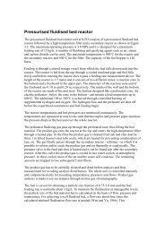
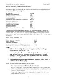
Single Stage CompressorThe SMI rig as described by Chriss [20] has been analyzedwith T-AXI and designed with T-C_DES. Figures 2 and 3show the rig cross section and the measured stage characteristicrespectfully. Table 1 lists the parameters that define this stagedesign. The 3D solution for the close wake generatorconfiguration was used to create the walls and stack file for theT-AXI calculation. The inputs for the one stage design in T-C_DES are in Tables 2 and 3. These design parameters wereset based on the measured flow rate and wheel speed as well ascomparing to the geometry of the actual hardware. The overallresults are in Table 4. The T-AXI results assume a good designexecution. The comparison between the two T-AXI runs isvery similar. It is not known why the measured efficiency wasso much lower than the T-AXI calculation.Figure 4 shows the initial T-AXI grid for the one stagedesign as well as the T-AXI screens during the different runs.The initial screen shows the input angular momentum. WithEuler’s Turbomachinery equation, the enthalpy rise iscalculated.The boundary layers are turned on once the solution isconverged with the loss model.Figure 2. Stage Matching Investigation rig crosssection(from Chriss [20].Figure 3. SMI measured overall stage characteristicfor the “clean” inlet and 40 wake generatorconfigurations (from Chriss [20]).Table 1. SMI Aerodynamic Design Parameters (fromChriss [20]).Parameter Rotor StatorNumber of airfoils 33 49Aspect Ratio - average 0.961 0.892Inlet Hub/Tip Ratio 0.75 0.816Flow/Annulus Area, lbm/sec/ft^2 40Flow/Frontal Area, lbm/sec/ft^2 17.502Flow Rate, lbm/sec 34.46Tip Speed, Correcte (ft/sec) 1120Mrel, LE Hub 0.963 0.82Mrel, LE Tip 1.191 0.69PR, Rotor 1.88PR, Stage 1.84D factor, Hub 0.545 0.502D factor, Tip 0.53 0.491LE Tip Diameter, in. 19 19LE Hub Diameter, in. 14.25 15.502Table 2. Stage data for one stage design (stage.smides).Parameter Stage 1Stage rotor inlet angle [deg] 0Stage rotor inlet Mach no. 0.5635Total Temperature Rise [K] 61.38Rotor loss coef. 0.076Stator loss coef. 0.04Rotor Solidity 1.892Stator Solidity 1.838Stage Exit Blockage 1Stage bleed [%] 0Rotor Aspect Ratio 0.69Stator Aspect Ratio 0.84Rotor Axial Velocity Ratio 0.863Rotor Row Space Coef. 0.07Stator Row Space Coef. 0.05Table 3, Initial data for one stage design (init.smides).Number of Stages 1Mass Flow Rate [kg/s] 15.631Rotor Angular Velocity [rpm] 13,508.92Inlet Total Pressure [Pa] 101,353Inlet Total Temperature [K] 288.167Alpha 3 - Last Stage [deg] -2.5Mach 3 - Last Stage 0.458Ratio of Specific Heats 1.4Gas Constant [kJ/kg*K] 0.28704Clearance Ratio 0.00158Tip Radius [m] 0.24137 Copyright © 2006 by ASME

Table 4. Performance Data for SMI example.SMIOverallGoalSMI "clean"measurementT-AXIcalculationwith SMIflowpathT-AXIcalculation forfree-vortexdesignTemperatureRatio 1.213 1.213PressureRatio 1.84 1.8 1.865 1.863Efficiency 87 91.53 91.37momentum and the real leading and trailing edge shapes areapplied from the 3D solution.Figure 7 shows how the T-C_DES design compares to theactual flowpath of the SMI stage.a.) Initial T-AXI grid showing bladeedge stations.b.) Initial screenTotal enthalpyc.) Screen after convergencewithout boundary layersAngularmomentumd.) Screen after convergencewith boundary layersentropyFigure 5. 3D representation of the one stage design.The Blade Viewer program can output all the bladesof a design.Boundary layer parametersFigure 4. T-AXI screens during the solution of theone stage design. Graphics are used to check inputand some guidance on solution convergence.Angular momentum is the primary input downstreamof each blade row. It is uniform for this free-vortexdesign.Figure 5 is a 3D representation of the stage design usingthe blade viewer. The max thickness to chord used is the sameas for rotor 1 and stator 1 of the EEE described in the nextsubsection. Figure 6 shows the T-AXI screen after the loss isconverged and the initial grid for the true SMI flowpath. Fromthese plots, it can be seen that the profiles of angularNASA/GE EEE 10 Stage CompressorThe NASA/GE EEE high pressure compressor wasdesigned during the late 1970’s using the best methodsavailable to industry at the time. A six stage build and two tenstage builds were used to refine the design [23,24]. Figure 8 isa cross section of the EEE HPC. This 10 stage design wasscaled up in size to become the high pressure compressor forthe GE90.T-C_DES was used to create geometry similar to the actualEEE flowpath. Reference [23] contains output from the GEaxisymmetric code, CAFD, which was used to construct theactual EEE flowpath and blade row angular momentumdistributions. Table 5 was initially constructed from themeanline data shown in Figures 10-14, and 17 in ref [23]. Thethroughflow information was used to get the axial velocityratios. The individual stage total temperature rise values wereadjusted to match the overall temperature ratio from the actualEEE T-AXI calculation. The losses were modified to get anoverall pressure ratio from T-C_DES of 25. The rotor inletMach number values were tweaked to get the stage rotorleading edge hub locations to match up with the actual design.The blockage was set based on the report that stated an inlet8 Copyright © 2006 by ASME

value of 0.97 and an exit value of 0.90 with an approximatelylinear distribution. This blockage is a very important parameterfor compressor design. It is used for sizing the area through thecompressor, and the coupled boundary layer in T-AXI is usedto approximate it. The aspect ratios and blade row gaps wereset to get approximately the right axial extent of each blade rowand stage. The stage tip radii are the values from the rotorleading edge of the actual flowpath. The bleed values werethose specified in the report, and applied as a negative blockagein T-AXI. Finally the solidity values were set to get the sameairfoil count as the actual EEE design.Angular momentuma.) T-AXI screen after loss is converged,but without boundary layers.b.) Initial T-AXI grid showingblade edge stations.Figure 6. T-AXI screens during the solution of theSMI case derived from the 3D simulation. Thissolution had contoured leading and trailing edges aswell as profiles of angular momentum.Actual 3D geometryFrom T-C_DESFigure 7. Comparison of the one stage flowpathgenerated with T-C_DES and the SMI geometry.Also shown are the leading edge and trailing edgestations.Figure 8. GE EEE High Pressure Compressor.The initial data and IGV data are in Tables 6 and 7respectively and come from the design intent. The clearancecomes from the clearance goals for the front rotors. The ratioof specific heat is treated as a constant in T-AXI. The valueused is the average of the value from the inlet TT and theexpected exit TT.Figure 9 shows the T-AXI screens for the 10 stage design.The distribution of angular momentum, total enthalpy, blockageand entropy are shown. The angular momentum plots give aquick picture to the user that the work and stator exit angleshave been input correctly. For the EEE, as mentioned in thedesign report, the large reduction in temperature drop in stage 6shown in Table 6 is to reduce the loading of that stage since thestator upstream is the last variable stator row. Although T-AXIcannot be used for off-design calculations, these designfeatures can be built into the parameters to address stall marginat part power. The distribution of rotor inlet angle (the same asthe upstream stator exit angle), also in Table 5, allows for agradual build-up of inlet rotor swirl for improved efficiencyand making sure the last stage stator or OGV is not too loaded.Figure 10 shows the T-AXI screens for the actual EEEHPC geometry. The edge stations for stage 10 demonstrate thenonlinear edge stations for the actual design. Figure 11compares the 10 stage design flowpath with the actual EEEflowpath demonstrating that the parameters available within T-C_DES are flexible enough to create a realistic flowpath.The thickness distributions in Table 8 have been applied tothe 10 stage design. They came from the actual EEE report[23]. Figure 12 demonstrates how the blade geometrycapability within T-AXI can be used. Fig. 12 a) shows a 3Dsolid of the airfoil, b) shows the converged MISES grid for themid-span section, c) shows the Mach number distribution, alsofor the mid-span section. Fig. 12 d) is a contour plot of theMISES Mach numbers and e) demonstrates how the “PressureEditor” capability in MISES, EDP, was used to smooth out thesuction side leading edge spike. A 3D representation of the 10stage design as output by the Blade Viewer is shown in Figure13.The overall performance calculations are shown in Tables9 and 10. The efficiency goal of the EEE was 85.7%. The two10 stage builds did not reach 100% speed, or that efficiencygoal. The T-AXI solution of the actual EEE flowpath withprofiles of angular momentum calculates an efficiency of9 Copyright © 2006 by ASME

Table 5. Stage data for 10 stage design (stage.e3c-des).StageParameter 1 2 3 4 5 6 7 8 9 10Stage rotor inlet angle [deg] 10.3 13.5 15.8 18 19.2 19.3 16.3 15 13.6 13.4Stage rotor inlet Mach no. 0.59 0.51 0.475 0.46 0.443 0.418 0.402 0.383 0.35 0.313Total Temperature Rise [K] 52.70 52.30 51.12 49.74 49.14 43.62 45.69 47.27 48.26 47.57Rotor loss coef. 0.053 0.0684 0.0684 0.0689 0.069 0.069 0.069 0.069 0.069 0.07Stator loss coef. 0.07 0.065 0.065 0.06 0.06 0.065 0.065 0.065 0.065 0.1Rotor Solidity 1.666 1.486 1.447 1.38 1.274 1.257 1.31 1.317 1.326 1.391Stator Solidity 1.353 1.277 1.308 1.281 1.374 1.474 1.379 1.276 1.346 1.453Stage Exit Blockage 0.963 0.956 0.949 0.942 0.935 0.928 0.921 0.914 0.907 0.9Stage bleed [%] 0 0 0 0 1.3 0 2.3 0 0 0Rotor Aspect Ratio 2.354 2.517 2.33 2.145 2.061 2.028 1.62 1.417 1.338 1.361Stator Aspect Ratio 3.024 2.98 2.53 2.21 2.005 1.638 1.355 1.16 1.142 1.106Rotor Axial Velocity Ratio 0.863 0.876 0.909 0.917 0.932 0.947 0.971 0.967 0.98 0.99Rotor Row Space Coef. 0.296 0.4 0.41 0.476 0.39 0.482 0.515 0.58 0.64 0.72Stator Row Space Coef. 0.32 0.35 0.45 0.45 0.9 0.46 0.89 0.52 0.58 0.55Stage Tip radius [m] 0.351 0.336 0.328 0.321 0.315 0.308 0.304 0.300 0.297 0.29584.6% whereas the Build 2 adjusted peak efficiency was84.8%. The 10 stage free vortex design solution has acalculated value of efficiency of 85.6%. These comparisonsare excellent for these calculations.a.) Initial T-AXI grid showing blade edgestations.Table 6. Initial data for 10 stage design (init.e3c-des).Number of Stages 10Mass Flow Rate [kg/s] 54.4Rotor Angular Velocity [rpm] 12,299.49Inlet Total Pressure [Pa] 101,325Inlet Total Temperature [K] 288.15Alpha 3 - Last Stage [deg] 0Mach 3 - Last Stage 0.272Ratio of Specific Heats 1.37836Gas Constant [kJ/kg*K] 0.287Clearance Ratio 0.0015b.)screenInitialTotal enthalpyAngularmomentumc.) Screen afterconvergencewithoutboundaryBlockageTable 7. IGV data for 10 stage design (igv.e3c-des).Soldity 0.6776Aspect ratio 5.133Phi Loss Coef. 0.039Inlet Angle 0Inlet Mach 0.47Lambda 0.97IGV Row Space Coef. 0.4IGV Tip Radius [m] 0.36211Boundary layerparametersd.) Screen afterconvergence withboundary layersEntropyFigure 9. T-AXI screens during the solution of the 10stage design. Graphics are used to check input andhelp guide solution convergence. Angularmomentum is the primary input downstream of eachblade row. It is uniform for this free-vortex design.10 Copyright © 2006 by ASME

Table 8. Maximum Thickness to chord data at huband casing for the GE EEE HPC applied to the 10stage design.Rotor 10a.) Initial T-AXI grid showing blade edge stations.Stator 10b.) Blow up of the Stage 10 grid showing details of the axisymmetricshape of the leading and trailing edge stations.Angular momentumc.) T-AXI screen after loss is converged, but without boundary layers.Figure 10. T-AXI screens during the solution of theEEE full geometry. This solution had contouredleading and trailing edges as well as profiles ofangular momentum as defined by the axisymmetricoutput in the EEE report.From T-C_DESActual 3D geometryFigure 11. Comparison of the 10 stage flowpathgenerated with T-C_DES and the EEE design. Alsoshown are the rotor 1 leading edge and stator 10trailing edge.Blade Row TM/C hub TM/C tipIGV 0.0850 0.0850R1 0.0961 0.0250S1 0.0599 0.1128R2 0.0849 0.0260S2 0.0462 0.0958R3 0.1085 0.0261S3 0.0626 0.0898R4 0.0813 0.0335S4 0.0666 0.0998R5 0.0799 0.0340S5 0.0703 0.0999R6 0.0797 0.0359S6 0.0730 0.1090R7 0.0960 0.0390S7 0.0671 0.0949R8 0.0786 0.0380S8 0.0799 0.1000R9 0.0741 0.0390S9 0.0799 0.1000R10 0.0850 0.0435S10 0.0601 0.0750Table 9. Comparison of the EEE efficiency goals andmeasurements with the T-AXI calculation results.EEE goalEEE Build 1Peak AdjustedEfficiency at97.5% speedEEE Build 2Peak AdjustedEfficiency at99% speedT-AXIcalculationfor EEEflowpathT-AXIcalculationfor 10 stageDesign withfree-vortex85.7 83.9 84.8 84.6 85.6NASA/GE EEE 5 Stage Low Pressure TurbineThe NASA/GE EEE 5 stage low pressure turbine is used todemonstrate the turbine capability in T-AXI and the turbinedesign capability of T-T_DES. In the first case, the Turbine setup code T-2-T-AXI was used to create a “walls” and “stack”file from the flowpath geometry, the initial data in Table 11,and the blade row data in Table 12. The work split waspresented in the NASA report [26], and adjusted to get theoverall temperature rise of 133.33 K as indicated by the designpoint test reading 503. This work split and the nozzle exitangles were used to get the angular momentum for each bladerow. This LPT case was also used by Reed and Turner [27] inthe validation of an entropy-based meanline code. Figure 14 isa cross section of the 5 stage EEE LPT.Figure 15 shows the initial grid, and Figure 16 shows theT-AXI screen after the loss is converged. The boundary layersare not applied for this turbine since the favorable pressuregradient makes its impact minimal.11 Copyright © 2006 by ASME

.) MISES grid of the Stator 7 midspansection,a.) Stator 7 geometry generated with T-AXI.c.) Stator 7 mid-span sectionanalyzed with MISES.d.) Stator 7 mid-span sectionMach number contours fromMISES solution.Figure 13. 3D representation of the 10 stage design. TheBlade Viewer program can output all the blades of a design.Figure 17 is a 3D representation of the LPT analyzed. Therequired input of max thickness to chord ratio was set to 5%.The turbine design code, T-T_DES used the initial data inTable 11 and the Stage data in Table 13 to create a 5 stagedesign that matched the flowpath of the EEE as shown inFigure 18 which is compared to the actual EEE flowpath.Notice how the flexibility of these parameters can be used tocome very close to an existing design. Table 14 shows theoverall result of the two T-AXI runs compared to the test data.e.) Stator 7 mid-span section modified with “PressureEditor” capability in MISES.Figure 12. Blade design features. The output ofgeometry and MISES files allows MISES to be runwithout changing files. With a small modification ofthe files, a coupled boundary layer can be run or amixed-inverse can allow a blade row section to beredesigned.Table 10. Comparison of the EEE goals with the T-AXI calculation results.EEE GoalT-AXIcalculation forEEE flowpathT-AXI calculation forDesign with freevortexTemperature Ratio 2.686 2.686Pressure Ratio 25 25.26 25.93Table 11. Initial Data for 5 stage EEE LPT matchingReading 503 from Block II Configuration 5 (fromBridgeman [26]) (init.lpt-des).Number of Stages 5Mass Flow Rate [kg/s] 28.321Rotor Angular Velocity [rpm] 3214.57Inlet Total Pressure [Pa] 310,801.3Inlet Total Temperature [K] 417.94Nozzle 1 Leading Edge Mach Number 0.335Inlet Duct Length/N1 Axial Width Ratio 1.441Ratio of Specific Heats 1.39689Gas Constant [KJ/(kg-K)] 0.287Clearance Ratio 0.000912 Copyright © 2006 by ASME

Table 12. Number of blades and hub tangentialvelocity (specifies angular momentum) for each bladerow.BladerowNumberof bladeshub Vtheta(ft/sec)N1 72 800R1 120 -388.214N2 102 820R2 122 -404.072N3 96 820R3 122 -391.928N4 114 780R4 156 -247.716N5 120 640R5 110 -103.938Figure 15. Initial grid for the 5 stage EEE LPT alsoshowing the leading and trailing edge stations.Figure 14. GE EEE LP Turbine Flowpath (fromBridgemann [26]) .Figure 16. T-AXI screen during the solution of the 5 stageEEE LPT.13 Copyright © 2006 by ASME

generate a 3D model allows blade weights to be calculated, andit is very rewarding to visualize the design in 3D.From the design system that has been described, a studentcan make the connection of key physical input parameters suchas Mach number and angle with the cross sectional area andangular momentum. Because angular momentum is a primaryquantity, its connection to the work is made obvious, and theability of a blade-to-blade solver to be connected directly canpresent the connection of loading with a change in angularmomentum. These concepts become second nature to thoseexperienced in turbomachinery, but it is useful when explainingto students to have a design tool that makes these connectionsmore obvious.Figure 17. 3D representation of the 5 stage LPTanalyzed. Blades were generated with 5% maxthickness to chord ratio.USE AS A TEACHING TOOLThe T-AXI suite of codes is meant to be used as part of asenior undergraduate or graduate level class, or as part of aresearch project. This paper has presented the overall theory ofthe codes and the validation using a single stage transoniccompressor, a 10 stage high pressure compressor and a 5 stagelow pressure turbine. Although not extensive, this validationprovides a level of trust that the design system results can beused in a design process. The input files can be easily modifiedto quickly change a design. The tables can be read into aspreadsheet program such as Excel, modified and output. Itbecomes a very easy process to add stages to create a 14 stageHPC design, for example. The files output by Excel can thenbe read by the design codes T-C_DES or T-T_DES. Asdemonstrated, the input parameters are flexible enough togenerate the flowpath for existing designs and therefore allowfor an almost unrestricted design space.The stage work input is easily specified through thetemperature rise or drop. Using many of the parameters for theEEE cases for loss, aspect ratio, or blade row spacing builds ona successful design. A new design can be configured to meet adesign condition, or an existing design can be reverseengineeredand validated to add to the database of cases. It isrelatively easy to create a good design, and the codes could betied to an optimizer to create an optimum design.The ability to easily couple with a blade-to-blade solversuch as MISES can be used for more advanced classes oradvanced projects. This allows for a complete demonstrationof the process so that calculated blade pressure profiles can beconnected to the blade loading parameters. The ability toCONCLUSIONS AND CODE ACCESSThe turbomachinery design system, T-AXI, has beenpresented and described with real multistage compressor andturbine examples. Three test cases have been used to validatethe method and loss models with good results. With a smallamount of input, a design can be created that is similar to a realdesign. The design is then defined by a small number ofparameters which can be used to explore the design space.This system is intended for use by educators and students toexplain turbomachinery concepts and for use in a design class.The system is also sophisticated enough for actual design use.Executable versions of the codes are available from theauthors’ web sites in addition to the input from the examplespresented and a user’s manual. The T-AXI web site URL’s are:http://gtsl.ase.uc.edu/T-AXI,http://web.mit.edu/merchant/www/taxi.html,andhttp://www.cfdg.unige.it/software.htm.Table 13. Stage Parameters for 5 stage design usingT-T_DES (stage.lpt-des); the temperature drop perstage came using work splits from Table IV ofBridgeman [26], and matching the overalltemperature rise of Reading 503.StageParameter 1 2 3 4 5Nozzle Exit Ang. [deg] 61 64.1 64.8 62.3 55.3Nozzle Exit Mach No. 0.5806 0.588 0.58 0.544 0.5Stage TT Drop [K] 27.53 29.797 30.944 26.474 18.583Nozzle Zweifel Number 0.639 0.956 0.978 1.058 1.075Rotor Zweifel Number 0.891 0.878 0.83 0.812 0.793Nozzle Loss Coef. 0.08 0.05 0.05 0.05 0.05Rotor Loss Coef. 0.12 0.1 0.1 0.1 0.05Nozzle Aspect Ratio 1.8106 3.5 3.77 4.94 5.47Rotor Aspect Ratio 4.088 4.57 5.38 7.76 6.05Rotor Axial Vel. Ratio 0.85 0.989 1.029 1.051 1Noz. Row Space Coef. 0.231 0.38 0.3 0.51 0.34Rotor Row Space Coef. 0.575 0.47 0.472 0.63 0.567Noz. Mean Radius [m] 0.2466 0.2729 0.2939 0.3141 0.3223Rotor Mean Radius [m] 0.2631 0.2845 0.3071 0.3203 0.319914 Copyright © 2006 by ASME

Radius (cm)4540353025201510-5 0 5 10 15 20 25 30 35 40 45Axial distance (cm)Table 14. Performance comparison between reading503 and the T-AXI calculations.T-AXIcalculationEEEflowpathHub EEETip EEEHub T-T_DESTip T-T_DESFigure 18. Comparison of the flowpath generatedwith T-T_DES using the stage input parameterscompared with the actual EEE 5 stage flowpath.MeasurementReading 503Pressure Ratio 4.409 4.351 4.326Temperature Ratio 1.468 1.464 1.463Efficiency 92.05 92.85 92.91T-AXI calculation(T-T_DES design)REFERENCES[1] Mattingly, Jack D., William H. Heiser, and David T. Pratt, AircraftEngine Design Second Edition, AIAA Education Series, Reston, VA,2002. Older versions of software in this book are available onthe web at www.aircraftenginedesign.com.[2] Mattingly, Jack D., Elements of Gas Turbine Propulsion, McGraw-Hill, AIAA Education Series, Reston, VA, 2005.[3] Genrup, Magnus, Ivan Carlsson, Ulf Engdar, and Mohsen Assadi,“A Reduced-Order Through-Flow Program for Choked and CooledAxial Turbines,” ASME Paper GT2005-68716.[4] Carlsson, Ivan, “A Reduced-Order Through-Flow Program forChoked and Cooled Axial Turbines,” MS Thesis for the Department ofHeat and Power Engineering Lund University, Lund, Sweden,February, 2005.[5] Merchant, A., Kerrebrock, J. L., Adamczyk, J.J., andBraunscheidel, E., “Experimental Investigation of a High PressureRatio Aspirated Fan Stage,” Journal of Turbomachinery, Vol. 127, No.1, pp. 43-51, January 2005.[6] Merchant, A., Epstein, A. H., and Kerrebrock, J. L., “Compressorswith Aspirated Flow Control and Counter-Rotation,” AIAA-2004-2514, 2nd AIAA Flow Control Conference, Portland, Oregon, June 28-1, 2004.[7] Smith, L. H. Jr., “The Radial-Equilibrium Equation ofTurbomachinery,” J. of Engineering for Power, pp 1-11, Jan. 1966.[8] Novak, R. A., “Streamline Curvature Computing Procedures forFluid-Flow Problems,” J. of Engineering for Power, pp 1-13, Jan.1966.[9] Drela, M. and M.B. Giles, “Viscous-Inviscid Analysis of Transonicand Low Reynolds Number Airfoils,” AIAA Journal, 25(10):1347–1355, Oct 1987.[10] Youngren, H.H. and M. Drela, “Viscous/Inviscid Method forPreliminary Design of Transonic Cascades,” AIAA-91-2364, 1991.[11] Adkins, G. G., Jr., and L.H. Smith, Jr., “Spanwise Mixing inAxial-Flow Turbomachines,” J. of Engineering for Power, Jan. 1982,Vol. 104, pp.97-110, also ASME paper 81-GT-57.[12] Koller, Ulf, Reinhard Monig, Bernhard Kusters, and Heinz-AdolfSchreiber, “Development of Advanced Compressor Airfoils forHeavy-Duty Gas Turbines--- Part I: Design and Optimization,” Journalof Turbomachinery Vol. 122, Issue 3, pp. 397-405, 2000. (Also ASME99-GT-95).[13] Küsters, B., Heinz-Adolf Schreiber, Ulf Köller, and ReinhardMönig, “Development of Advanced Compressor Airfoils for Heavy-Duty Gas Turbines— Part II: Experimental and Theoretical Analysis,”Journal of Turbomachinery -- July 2000 -- Volume 122, Issue 3, pp.406-414. (Also ASME 99-GT-96).[14] Zweifel, O., “The Spacing of Turbomachine Blading, Especiallywith Large Angular Deflection,” Brown Boveri Review 32, 1945.[15] Hirsch, C.H. and J. D. Denton Editors, “Axial CompressorPerformance Predictions,” in “Throughflow Calculations in AxialTurbomachines,” 1981. AGARD-AR-175.[16] Koch, C.C. and L.H. Jr. Smith, “Loss Sources and Magnitudes inAxial Flow Compressors,” Journal of Engineering for Power, pages411–424, July 1976.[17] Denton, J.D., “Loss Mechanisms in Turbomachines,” J. ofTurbomachinery, Vol 115, pg 621-656, October 1993.[18] Leiblein, S., F.C. Schwenk, and F.L. Broderick. “Diffusion Factorfor Estimating Losses and Limiting Blade Loadings in Axial FlowCompressor Blade Elements,” Tech. Report RME53D01, NACA,1953.[19] Ucer, A.S., Stow, P., and Hirsch, Ch., (Editors),“Thermodynamics and Fluid Mechanics of Turbomachinery,” VolumeII, NATO ASI Series, 1985.[20] Chriss, Randall M., William W. Copenhaver and Steven E.Gorrell, “The Effects of Blade-Row Spacing on the Flow Capacity ofa Transonic Rotor,” ASME paper 99-GT-209., June, 1999.[21] Turner, Mark G., Steven E. Gorrell, and David Car, “RadialMigration of Shed Vortices in a Transonic Rotor Following A WakeGenerator: A Comparison Between Time Accurate and AveragePassage Approach,” ASME Paper No. GT2005-68776, Reno, June2005.15 Copyright © 2006 by ASME

[22] Gorrell, S. E., Car, D., Puterbaugh, S. L., Estevadeordal, J., andOkiishi, T. H., “An Investigation of Wake-Shock Interactions in aTransonic Compressor with DPIV and Time-Accurate CFD,” ASMEpaper GT2005-69107, Reno, NV, 2005.[23] Holloway, P.R., G.L. Knight, C.C. Koch, and S.J. Shaffer,“Energy Efficient Engine High Pressure Compressor Detail DesignReport,” NASA CR-165558, 1982.[24] Cline, S.J., W. Fessler, H.S. Liu, R.C. Lovell, and S.J. Shaffer,“High Pressure Compressor Component Performance Report,” NASACR-168245, 1983.[25] Cherry, D.G., C.H. Gay, and D.T. Lenahan, “Low PressureTurbine Test Hardware Detailed Design Report,” NASA CR-167956,1982.[26] Bridgeman, M.J., D.G. Cherry, and J. Pedersen, “NASA/GEEnergy Efficient Engine Low Pressure Turbine Scaled Test VehiclePerformance Report,” NASA CR-168290, 1983.[27] Reed, John A., and Mark G. Turner, “An Entropy Loss ApproachFor A Meanline Bladerow Model With Coupling To Test Data and 3DCFD Results,” ASME Paper No. GT2005-68608, Reno, June 2005.16 Copyright © 2006 by ASME