High-frequency restoration of surface seismic data - Arcis

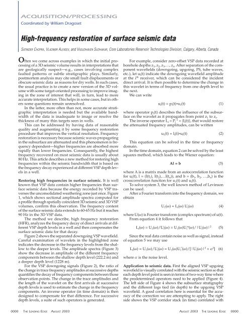
ACQUISITION/PROCESSINGCoordinated by William DragosetHigh-frequency restoration of surface seismic dataSATINDER CHOPRA, VLADIMIR ALEXEEV, and VASUDHAVEN SUDHAKAR, Core Laboratories Reservoir Technologies Division, Calgary, Alberta, CanadaOften we come across examples in which the initial processingof a 3D seismic volume results in interpretations thatare geologically suspect—e.g., cases involving complexfaulted patterns or subtle stratigraphic plays. Similarly,postmortem analysis may cite small fault displacements orobscure seismic data as reasons for dry wells. In such cases,the usual practice is to create a new version of the 3D volumewith some target-oriented processing to improve imagingin the zone of interest that will, in turn, lead to moreaccurate interpretation. This helps in some cases, but in otherssome questions remain unresolved.In the latter, more often than not, more accurate stratigraphicinterpretation is needed but the available bandwidthof the data is inadequate to image or resolve thethickness of many thin targets seen in wells.This can be addressed by having data of reasonablequality and augmenting it by some frequency restorationprocedure that improves the vertical resolution. Frequencyrestoration is necessary because seismic waves propagatingin the subsurface are attenuated and this phenomenon is frequencydependent—higher frequencies are absorbed morerapidly than lower frequencies. Consequently, the highestfrequency recovered on most seismic data is usually about80 Hz. This article describes a new method for restoring highfrequencies within the seismic bandwidth that is based onthe frequency decay experienced at different VSP depth levelsin a well.Restoring high frequencies in surface seismic. It is wellknown that VSP data contain higher frequencies than surfaceseismic data because the energy recorded by VSP traversesthe unconsolidated weathering zone just once. Figure1, which shows sectional amplitude spectra computed fora profile through spatially coincident 3D seismic and 3D VSPvolumes, confirm this observation. The frequency contentof the surface seismic data extends to 60-65 Hz but it reaches90 Hz in the 3D VSP data.The method we describe, high frequency restoration(HFR), analyzes the frequency decay of direct arrivals at differentVSP depth levels in a well and then compensates thesurface seismic data for that decay.Figure 2 shows the separated downgoing VSP wavefield.Careful examination of wavelets in the highlighted zoneindicates the decrease in the frequency levels from the shallowto the deeper levels. The amplitude spectra (Figure 3)show the decrease in amplitude of the different frequencycomponents between the shallow depth level (222.2 m) anda deeper depth level (1228 m).For the VSP downgoing signals (Figure 2), the ratio ofthe change in trace frequency amplitudes at successive depthsquantifies the decay of frequency components between thoseobservation points. The change in the trace amplitudes andthe length of the wavelet on the first arrivals at successivedepth levels is used to estimate the change in the frequencycomponents. An inverse operator (in time domain) is thendesigned to compensate for that difference. For successivedepth levels, a suite of such operators is generated.For example, consider zero-offset VSP data recorded atborehole depths z 1 , z 2 , z 3 ,…, z n . After separation of the componentwavefields (downgoing, upgoing, PS, tube waves,etc.), let u i (t) indicate the downgoing wavefield amplitudeat the i th receiver, which can be considered the incidentdirect arrival. It is then possible to determine the change inthis wavelet in terms of frequency from one depth level tothe next.We can writeu i (t) = p i (t)*u 1 (t) (1)where operator p i (t) describes the influence of the subsurfaceon the wavelet as it propagates from point z 1 to z i .The inverse operator L i = P i-1= {l i (t)}, that would restorethe attenuated frequency amplitudes, can be writtenu 1 (t) = l i (t)*u i (t) (2)This equation can be solved in the time or frequencydomain.In the time domain, equation 2 can be solved by the leastsquares method, which leads to the Wiener equation:Al = b (3)where A is a matrix made from an autocorrelation functionfor u i (t), l = (l(t 1 ), l(t 2 ),…l(t n )), and b = (b 1 , b 2 , …,b n ) is thecrosscorrelation function for u 1 (t) and u i (t).To solve system 3, the well known method of Levinsoncan be used.After a Fourier transform into the frequency domain, weobtainU 1 (ω) = L i (ω) U i (ω) (4)where U(ω) is Fourier transform (complex spectrum) of u(t).From equation 4 it follows thatL i (ω) = U 1 (ω)/U i (ω) = U 1 (ω)U i *(ω)/|U i (ω)| 2 (5)Since the real data contain noise as well as signal, insteadof equation 5 we may useL i (ω) = U 1 (ω)/U i (ω) = U 1 (ω)U i* (ω)/[|U i (ω)| 2 + α 2 ] (6)where α is the noise level.Application to seismic data. First the aligned VSP upgoingwavefield is visually correlated with the seismic section so thateach depth level point is seen in terms of two-way time wherethe predetermined operators need to be applied (Figure 4).The left side of Figure 4 shows the subsurface stratigraphyand the different logs tied (in depth) to the upgoing VSPwavefield. A good correlation here is essential for the accuracyof the correction we are attempting to apply. The rightside shows the VSP corridor stack (in time) correlated with0000 THE LEADING EDGE AUGUST 2003 AUGUST 2003 THE LEADING EDGE 0000

Figure 1.Sectional amplitudespectra of aprofile from surfaceseismic (left),and 3D VSP(right). Verticalaxis is frequency.Figure 2.Downgoingwavefieldobtained afterseparation ofcomponentwavefields fromthe VSP totalwavefield forwell 1.Figure 3.Amplitude spectraat a shallowand a deep depthlevel.0000 THE LEADING EDGE AUGUST 2003 AUGUST 2003 THE LEADING EDGE 0000

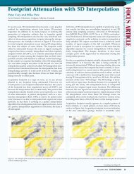
Figure 4. Correlation of stratigraphy, VSP upgoing wavefield, well logs, VSP corridor stack, and surface seismic data.Figure 5. Seismic inline 85 extracted out of a 3D seismic volume before (left) and after (right) HFR.logs, a filtered version of the corridor stack, and the seismicsection. The green lines indicate the depth-to-time matchingof individual formation tops seen on the logs and upgoingwavefield (in depth) with the surface seismic data. This fixesthe VSP upgoing wavefield extent or spread on the seismic.The first operator corresponding to the first depth level is nowassigned a starting time and so, in this way, each determinedoperator has a corresponding time node point application onthe seismic. Thereafter, the filter application is run (as convolutionin time domain) on the seismic data. As operators areapplied continuously to the stacked data, windowing isavoided. Application of these inverse operators on surface seismicdata enhance the frequency bandwidth by restoring theattenuated frequency components.0000 THE LEADING EDGE AUGUST 2003 AUGUST 2003 THE LEADING EDGE 0000

Figure 6. Sectional amplitude spectra for seismic inline 85 indicates the extent of frequency enhancement.Figure 7. Seismic crossline 72 before (left) and after (right) HFR.A3D VSP and a coincident 3D surface seismic surveywere recorded around well 8-20 in the Hanna area of centralAlberta, targeting the Lower Mannville formation (Chopra etal., 2002). The well encountered a gross Lower Mannvilleinterval 20.5 m thick and thicker than in adjacent wells 6-20(11.5 m) and 8-21 (7 m). The 3D seismic programs (surface andVSP) were recorded to assist in defining sand presence andporosity development in the Lower Mannville intervalbetween 1300 and 1350 m. The objectives for the 3D VSPrecording were to (a) tie the seismic reflections to lithologyand stratigraphic boundaries; (b) obtain a high frequencyimage around the borehole (the fixed receiver array and itsproximity to the reservoir are expected to improve imagequality); and (c) obtain an improved subsurface velocity model.HFR was run on the seismic data. Figure 5 shows a segmentof seismic inline 85 with and without HFR. Notice the0000 THE LEADING EDGE AUGUST 2003 AUGUST 2003 THE LEADING EDGE 0000

Figure 8. Sectional amplitude spectra for seismic crossline 72 before (left) and after (right) HFR.Figure 9. Overlay of a 3D VSP vertical plane and seismic (inline 85) after HFR.0000 THE LEADING EDGE AUGUST 2003 AUGUST 2003 THE LEADING EDGE 0000

Figure 11. Timeslices from thecoherence volumesbefore (left) andafter (right) HFR.Figure 12. Timeslices from thecoherence volumesbefore (left) andafter (right) HFR.Figure 13. (a)Segment of impedancesection.Highlighted portionindicateslower impedanceat the level of gassand but does notdistinguish it. (b)Segment of impedancesection.Highlighted portionindicates theextent of the gassand clearly.a)b)0000 THE LEADING EDGE AUGUST 2003 AUGUST 2003 THE LEADING EDGE 0000

a)Figure 14. (a) Operators derived from well 1.(b) Operators derived from well 2. (c)Difference of operators derived from wells 1and 2.b)c)For the same area, if the geology does not change abruptly,the HFR filters from different VSP surveys should be the same,(assuming data quality is good and is acquired using similarequipment). The set of inverse filters were computed fromVSPs in two different wells in the same field. The objectivewas to determine how different these sets of filters were.Figures 14a and 14b show the filters determined from two differentwells. Figure 14c shows their difference. Clearly, the filtersare almost identical. Such tests carried out on differentwells in different areas lead us to conclude that HFR is robust.However, in areas where geology changes fast laterally, a spatialadaptive filter application approach may be necessary.Prestack application of HFR. Application of HFR to poststackdata has been illustrated in the examples above. Applicationto prestack data is also very effective and useful for AVOanalysis. However, since a zero-offset VSP is used to determinethe attenuation in terms of a set of HFR filters, applicationto seismic gathers would mean application of the sameset of filters for all offset traces. Attempts at offset-dependentcorrection to gathers requires several walkaway VSPs fordetermining one set of HFR filters for each offset. This exercisehas been carried out with convincing results for AVOanalysis. This work is currently under way and will be presentedupon its completion.Conclusions. The HFR method described in this article differsfrom conventional industry methods. It consists of determiningthe frequency-dependent decay from downgoing VSPfirst arrivals from successive depth levels, and then applyingthe inverse decay function to surface seismic data. Advantagesof this procedure include:• poor reflection zones, resulting from strong impedancecontrasts above and below a particular zone of interest,show greater reflection detail and continuity and bettermatch corridor stacks or VSP offset sections• impedance inversion on data with HFR application, andhence higher bandwidth, show more detail and lead tomore detailed interpretation of important stratigraphicfeatures,• HFR methodology is robust.HFR helps define trends better and leads to more confidentinterpretations. Such applications could redefineprospects, which in some cases may have been declaredunsuccessful, when the interpretations are based on seismicdata with poor bandwidth.Suggested reading. “Simultaneous acquisition of 3D surfaceseismic and 3D VSP data—processing and integration” byChopra et al. (SEG 2002 Expanded Abstracts). “Fault interpretation—thecoherence cube and beyond” by Chopra and Sudhakar(Oil and Gas Journal, 2000). “Azimuth based coherence for detectingfaults and fractures” by Chopra et al. (World Oil, 2000).“Model-based Q compensation” by Hirsche et al. (SEG 1984Expanded Abstracts). TLEAcknowledgments: Coherence Cube and HFR are trademarks of CoreLaboratories. We are indebted to Bob Hardage and Rob Stewart for editingthe manuscript thoroughly and improving its quality. We thank JoanneLanteigne for formatting some images in this paper and Jan Dewar for hervaluable comments and suggestions. We thank ConocoPhillips Canada forrelease of data and Core Laboratories for permission to publish.Corresponding author: schopra@corelab.ca0000 THE LEADING EDGE AUGUST 2003 AUGUST 2003 THE LEADING EDGE 0000