Estimating the Water Requirements for Plants of Floodplain Wetlands

Estimating the WaterRequirements for Plantsof Floodplain Wetlands:a GuideJane Roberts, Bill Young and Frances Marston

Published by:Land and Water Resources Research and Development CorporationGPO Box 2182Canberra ACT 2601Telephone: (02) 6257 3379Facsimile: (02) 6257 3420Email: public@lwrrdc.gov.auWebSite: www.lwrrdc.gov.au© LWRRDCThis project was funded under the National River Health Program, managed by theLand and Water Resources Research and Development Corporation (LWRRDC) andEnvironment Australia. The program’s mission is to improve the management ofAustralia’s rivers and floodplains for their long-term health and ecologicalsustainability.Disclaimer:Publication data:Authors:The information contained in this publication has been published by LWRRDC toassist public knowledge and discussion and to help improve the sustainablemanagement of land, water and vegetation. Where technical information has beenprepared by or contributed by authors external to the Corporation, readers shouldcontact the author(s), and conduct their own enquiries, before making use of thatinformation.‘Estimating the water requirements for plants of floodplain wetlands: a guide’.Occasional Paper 04/00.Jane Roberts, Bill Young and Frances MarstonCSIRO Land & WaterPO Box 1666Canberra ACT 2601Telephone: (02) 6246 5763Facsimile: (02) 62460 5800E-mail: jane.roberts@cbr.clw.csiro.auISSN 1320-0992ISBN 0 642 76024 1Designed and typeset by Arawang Communication GroupPrinted by Union Offset Co. Pty LtdSeptember 2000

ContentsPreface 7Acknowledgments 8Guide to Contents 9Section 1: Introducing floodplain wetlands 9Section 2: Introducing the vegetation 9Section 3: A stepwise procedure 9Section 4: Old and new data 9Section 5: Obtaining vegetation data 10Section 6: Using water regime data 10Section 7: Predicting vegetation responses 10Section 1: Introducing Floodplain Wetlands 11What are floodplains? 11What are floodplain wetlands? 13Introducing the hydrology 13Water regime 15Section 2: Introducing the Vegetation 18Water as a part of the environment 18Floodplain vegetation 23Ecological groups 25Plant water regime 28Section 3: A Step-wise Procedure 33Outline 33Step 1: Describing the floodplain wetland 34Step 2: Setting management objectives 35Step 3: Vegetation–hydrology relationships 36Step 4: Determining the required water regime 37Step 5: The trade-off process 38Section 4: Old and New Data 40The evaluation process 40Evaluating existing information 40Options for new information 43Applications 48Section 5: Obtaining Vegetation Data 50Field methods and protocols 50What to use? 50Describing the vegetation 55Spatial issues 59Species-based relationships 61Special studies 62Section 6: Using Water Regime Data 65Estimating water depth 65Using storage volume and inundation area 66Estimating inundation areas 69Estimating storage volumes 71Contents 3

Factors affecting interpretation 78Modelling wetland water balance 80Australian examples 81Section 7: Predicting Vegetation Responses 84Simulation modelling 84Category 1: hydrologic/expert opinion 85Category 2: hydrologic/empirical 87Category 3: hydraulic/empirical 88Category 4: hydraulic/process 88Concluding Remarks 91References 92Web Listings 100Appendix 1: Remote Sensing 101Choice of application 101Inundation mapping 101Appendix 2: Evapotranspiration 109Evapotranspiration data 109List of Figures1 Floodplain features 122 Forms of floodplain wetlands 123 A floodplain wetland 134 Wanganella Swamps, southern New South Wales,July 1992 145 Wetland water regimes 156 Storage volume hydrographs 177 Vegetation zonation 198 Structural diversity 269 Aquatic growth-forms 2710 Wetland plant functional types 2811 Flow chart showing five steps for determining thethe water requirements of floodplain wetlands plants 3312 Vegetation–hydrology relationships 4313 Lippia, a floodplain weed 4614 Species versus community responses 5115 Range of tree condition within a species 5416 Spatial–temporal sequence 5617 Vigour in leafless species 5918 Heat pulse sensor 6419 Cracks after winter rains 6720 Crack volume and drying time 6821 The relationship between inundated area and storagevolume 7022 Antecedent conditions 7123 Commence-to-flow and inflow 7224 Degraded channel 80A1–1 Inundation-area curve 104A1–2 A visual expression of the information range andquality obtainable from remote sensing 1054 Estimating the Water Requirements for Plants of Floodplain Wetlands

List of Tables1 Spatial variability in dominant species and understorey 53A1–1 Sensor, cost, and suitability for floodplain wetlandmanagement 102A1–2 Specifications for sensors suitable for floodplain wetlandmanagement 103A1–3 Measured and predicted inundated area 106A1–4 A flooding overlay check 108A1–5 Comparison of two methods 108A2–1 K c and K s for plant communities typical of south-easternAustralia 109A2–2 Range of reference values, relative to well-wateredgrass 110Contents 5

PrefaceThroughout Australia, the future of water resources, water-dependentindustries and aquatic ecosystems is being reviewed. The principal usersof river water, that is industries and ecosystems, are being identified andtheir respective needs are being formally recognised. Although theprocess of making allocations differs between jurisdictions, there is acommon requirement for quantitative estimates of these needs. Atpresent, the allocation process is faced with uneven knowledge, andecosystem needs are inadequately articulated. This guide addresses theneeds of one part of the riverine ecosystem: the plants of floodplainwetlands.In terms of flow management, riverine ecosystems can be divided intoin-channel and over-bank or floodplain. The links between in-channelecology and flow regime are recognised and there has beenconsiderable development in defining and quantifying the in-streamflow needs. The recent publication of wetland books, reviews andmanuals shows a similar advance in understanding for single wetlands(Note A). In contrast, knowledge of the over-bank riverine environment,or whole floodplain complexes, has advanced much more slowly.Floodplain wetlands are large and diverse, but are typically wellvegetated.This vegetation has value as habitat providing, for example,refuge and breeding opportunities; these values are not fixed butchange through time. Because they support large waterbird populationsafter flooding, many floodplain wetlands have been listed as wetlands ofnational and international significance.In this guide we aim first, to advise on how to estimate the waterrequirements of the plants on these floodplain wetlands, and second toinform and thus increase understanding. It is not a prescriptive manual.As a guide, it is directed at persons charged with making decisionsabout water allocations, persons who are not necessarily trained in allrelevant areas.The guide draws on case histories from Australia, but is not a criticalreview. Most of the cases are from inland rivers in eastern Australia,where the pressures of agricultural development have been mostacutely felt.Restoration has been a management goal in wetland managementworldwide, but in Australia there has been a drive to restore a wetlandby restoring its ‘natural’ or pre-European water regime. This is possiblefor smaller, discrete wetlands, often with the aid of structures such asregulators, but is much harder to achieve for floodplain wetlands.Rehabilitation has been the primary management goal for the in-streamenvironment. Rehabilitation is the reality of managing heavily regulatedrivers where the goal is to obtain small improvements while workingwithin operational constraints. Resolution of what is desirable orachievable for floodplain wetlands is within the social and politicalsphere, and outside the frame of this guide, which instead outlinesapproaches suitable for restoration and rehabilitation.NOTE AOn wetland managementFor general reading on wetlandmanagement, see the range ofmanuals recently produced by Stateagencies across Australia. Examplesare:“Wetland management; a manual forwetlands of the River Murray inSouth Australia” (Carter andNicolson 1993)“Manual of wetlands management”(Hull and Beovich 1996).“Wetlands of the Swan Coastal Plain:their nature and management”(Balla 1994).These focus on individual wetlandsor discrete waterbodies, such asbillabongs, rather than on wetlandcomplexes.Some manuals include sections onwater management, and introducebasic hydrological concepts.Methods used for estimating waterrequirements of wetlands arereviewed in “Comparative evaluationof environmental flow assessmenttechniques: review of methods”(Arthington and Zalucki 1998): thisseparates ‘wetlands’ from‘floodplains’, and focuses onwetlands only.Preface 7

Note that the guide is concerned primarily with water quantity. Waterquality and land management, both of which are factors that canadversely affect the condition of plants on floodplain wetlands, are notconsidered.AcknowledgmentsThe development of this Guide was funded by the Land and WaterResources Research and Development Corporation (LWRRDC), underits National River Health Program, and supported by CSIRO Land andWater. The project Steering Committee, comprising Paul Wettin(DLWC), Laurie Olive (ADFA) and Peter Davies (LWRRDC), providedvaluable input and advice throughout the project.The authors would like to thank Peter Fairweather, Deakin University;Rob McCosker, LandMax; John Duggin, University of New England;Anthony Scott, CSIRO Land and Water, Canberra; and Greg Brereton andPaul Keyte, NSW Department of Land and Water Conservation, Dubbofor their assistance and discussions at various times.Specific contributions were made by Mick Fleming (evapotranspirationand infiltration) and Leo Lymburner (remote sensing techniques) ofCSIRO Land and Water, Canberra and their advice is gratefullyacknowledged.Finally, we would like to thank our reviewers for their comments: StuartBlanch (Inland Rivers Network), Max Finlayson (ERISS), Ray Froend(Edith Cowan University), P.M. Fleming (CSIRO Land and Water), ChrisGippel (University of Melbourne), and Paul Wettin and Greg Raisin(DLWC).8 Estimating the Water Requirements for Plants of Floodplain Wetlands

Guide to ContentsThe aim of this guide is to advise readers on how to go aboutestimating the water requirements of plants on floodplainwetlands. This is a multi-disciplinary task, drawing on expertise inhydrology and plant ecology. There is no reference text for this.The task is made more difficult because of the general lack ofinformation on floodplain hydrology, geomorphology andvegetation.Section 1: Introducing floodplain wetlandsUnderstanding floodplain geomorphology and hydrology is the key tounderstanding ecological diversity of floodplain wetlands, and tounderstanding the vegetation. In this section, the key features ofgeomorphology and hydrology are introduced, to show the diversitywithin and between floodplains. Floodplain water balance, which is animportant part of this guide, is also introduced, and its link to waterregime outlined.Section 2: Introducing the vegetationThis section gives an ecological background to floodplain vegetation, bylooking at some of the ways that water, and water regime, affect plants.First, water is considered as part of the plant environment anddescribed as environmental gradients across the floodplain; then it isconsidered as a resource; and finally as a resource and as anenvironment that affects other resources. Vegetation attributes that areroutinely used to describe terrestrial vegetation are presented, in thecontext of Australian floodplains. Descriptive approaches such asgrowth-forms and plant functional types are outlined in relation to thefloodplain environment. Plant water regime and its seven maincomponents are presented, and the value of focusing on depth isemphasised.Section 3: A stepwise procedureThe process for determining the water requirements for plants offloodplain wetlands can appear complicated and even circular to thoseinvolved in the process, but in fact it follows a series of well-definedsteps. These steps are similar regardless of political process or whichfloodplain wetland is being considered. This section describes the fivesteps in this general procedure. Only Step 3 and Step 4, both purelybiophysical, are treated in detail in this guide.Section 4: Old and new dataOne of the first decisions is whether to use existing vegetation–hydrology relationships, or to develop new ones. An assumption of thisguide is that existing hydrological data are likely to be adequate, so itGuide to Contents 9

ecomes a matter of how to use what water regime is available andhow to improve it. Nevertheless, it is likely that there will be few usefulvegetation data, so they will have to be collected. This section discusseshow to evaluate existing knowledge, then outlines options fordeveloping new relationships, based on field studies. There is a definiterole for special studies and experimental research, which tend to beoverlooked.Section 5: Obtaining vegetation dataWhen there is little or no previous information about water regime forrelevant species, then vegetation–hydrology relationships must beestablished from scratch. This section describes what sort of vegetationdata to obtain, and whether to do this at the level of species orcommunity; if at species level, ways of choosing species are outlined.Different measures of vegetation are described — abundance, characterand vigour — and examples given for species, community and differentgrowth-forms. Techniques for measuring abundance, character, andhealth are outlined, rather than given in detail. Examples are given ofAustralian studies and experiments to show how these complement afield-based vegetation–hydrology relationship.Section 6: Using water regime dataThe hydrologic variable of most relevance to plants is water depth, butwater depth data are rarely available for large wetlands. Depth can beobtained directly, or indirectly by water balance calculations fromexisting data. This section focuses on the indirect ways for obtainingdepth, but recognises that water regime can be defined in other ways.Options for estimating the different components of a floodplainwetland water balance are described, with emphasis on spatial andtemporal variations across the floodplain wetland. The application ofwater regime data for hydrological modelling is described, with currentAustralian examples, although these are rarely based on depth.Section 7: Predicting vegetation responsesThe general procedure advocated in this guide is to use vegetation–hydrology relationships to predict the likely future state of floodplainwetland vegetation as a result of proposed changes to water regime.The process of making these predictions is referred to as modelling.While modelling may be as simple as expert predictions based on aconceptual model, in general it involves repetitive calculations todescribe the temporal and or spatial patterns in vegetation response.This section identifies four different categories of modelling, basedloosely on the complexity of the modelling approaches, and describesthem using examples from Australia and North America.10 Estimating the Water Requirements for Plants of Floodplain Wetlands

Section 1:IntroducingFloodplainWetlandsUnderstanding floodplain geomorphology and hydrology is thekey to understanding ecological diversity of floodplain wetlands,and for understanding the vegetation. In this section, the keyfeatures of geomorphology and hydrology are introduced, toshow the diversity within and between floodplains. Floodplainwater balance, which is an important topic of this guide, is alsointroduced, and its link to water regime outlined.What are floodplains?Floodplains are fluvial depositional environments formed over longperiods from sediments transported by rivers in flood. In terms of riverflow velocity, floodplains are low energy environments, a result of theirvery low slopes and low relief (Note 1).The rate of floodplain formation depends on the prevailing flow regimein the river and on the nature of sediment delivery from the uppercatchment. Most floodplains are polyphasic ie. they have been formedunder variable flow, climate and deposition conditions, whereas amonophasic floodplain is one formed under just one set of conditions.Old floodplains are unlikely to be monophasic, but young ones mightbe. The age of floodplains varies. The Willandra Lakes on the LachlanRiver distributary are at least 55,000 years old, whereas coastalfloodplains of the Northern Territory are 3–6,000 years old. Anappreciation of the age of a floodplain and its forms is useful forunderstanding its ecological diversity. Floodplains on large rivers arelarge, covering 100,000–200,000 hectares.Fluvial forms on floodplain wetlands are mainly relict channelfeatures, such as billabongs and anabranches (eg. Figure 1). Billabongs,which include ox-bows, cut-off meanders and small lentic features, canbe numerous and quite diverse. If billabongs originate from a period ofhigher discharge, their dimensions will exceed those of thecontemporary river, and they will have different sedimentcharacteristics. Floodplain age and formation can be a short guide tobillabong diversity. Anabranches are channels that leave then re-join thepresent river. Typically, these flow at times of high discharge. Often, butnot always, an anabranch is a paleochannel and its dimensions aredifferent from the present river. Anabranches are a notable feature of themajor rivers in the Murray–Darling system.Note 1Floodplain classificationLack of scientific and ecologicalstudies of floodplains have hinderedunderstanding of floodplain ecology.An example of this is that as yet thereis no Australia-wide system offloodplain classification.In general, the most effectiveclassification systems are those thatare based on their formativeprocesses, also known as functionalor genetic classifications. Forfloodplains, this means aclassification system based on streampower, discharge and sedimentcharacteristics.A genetic floodplain classificationsystem has been developed byNanson and Croke (1992). TheirClass C, low-energy cohesivefloodplains, covers terminal wetlandsand most of the floodplains in theMurray–Darling Basin.Section 1: Introducing Floodplain Wetlands 11

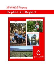
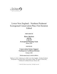
Figure 1. Floodplain featuresThe floodplain of a lowland alluvialriver in the southern Murray–DarlingBasin. Both fluvial and non-fluvialfeatures are evident: see the relictchannels and the dune. Non-fluvialfeatures typically have distinctive soilsor lithology: if elevated, as shownhere, these features serve asecological islands, increasing regionaldiversity and acting as a refuge inmajor floods.Non-fluvial forms on inland floodplains include aeolian features suchas dunes and shallow deflation basins with their distinctive quasicircularshape and accompanying lunette on the downwind side.The width of the floodplain generally increases in the downstreamdirection as the river valley widens. In the middle reaches of mostalluvial rivers, the floodplain is bounded by valley walls that constrainfloods, so most floodwater returns to the main river channel. Thelowest reaches of alluvial rivers are usually beyond the lateralconstraints of valley walls, so floodwaters spread out. Consequently,there is very little return to the main river channel, except in majorfloods. In this very low energy environment, the river virtually ceases.Such floodplains are described in this guide as terminal. These terminalfloodplains may take different forms, such as an alluvial fan or delta,with a slightly concave cross-section and a divergent distributarychannel network, or may be basin-like (Figure 2). (Understandingfloodplain form and whether it is confined or not helps to understandfloodplain hydrology, surface topography and its variability, thedistribution of floodwaters, and ecological complexity.) Confinedfloodplains, then, are where a flood exiting the upper river reachesslows down and spreads out, but is bounded by valley walls; the lowerunconfined floodplain can be considered as where the flood dissipates.On long rivers, confined floodplains are steeper on the upper plainswhere the rivers exit from the uplands; and flatter further downstream.The upper and lower confined floodplains are therefore differentiatedby valley slope.Figure 2. Forms of floodplain wetlandsSchematic diagram showing some types of floodplain wetlands. From left to right, two types of confined floodplains,and three unconfined and terminal floodplains, with little through-flow. Floodplains with braided channels are morefragmented and more complex than basin-like ones. All these are found in the Murray–Darling Basin.ImpededBraidedDelta/FanConfinedBasin12 Estimating the Water Requirements for Plants of Floodplain Wetlands

Understanding floodplain form and whether it is confined or not helpsto understand floodplain hydrology, surface topography and itsvariability, the distribution of floodwaters, and ecological complexity.What are floodplain wetlands?In this guide, a floodplain wetland refers to the whole floodplainsurface, so includes fluvial and non-fluvial features (Figure 1); ‘wetland’(Note 2) refers to those areas that retain water, and ‘floodplain’ refers tothose areas that drain readily (Figure 3). This is an ecologicalperspective: geomorphologists would refer to these areas as afloodplain.Figure 3. A floodplain wetlandA cross-section through one side of a confined floodplain, showing howfloodplain wetland refers to a mosaic of floodplain and wetland habitats.RiverRiverbankFloodplainWetlandWetlandCut-off meandersRiverchannelFloodplainPaleo channelor anabranchThe different-aged fluvial forms described above provide a range ofwater-holding areas on the floodplain, and hence a diversity of wetlands.A floodplain wetland is therefore a complex or a mosaic of wetlands andfloodplains, and of water regimes, and hence habitat types forvegetation.Introducing the hydrologyThe hydrology of a floodplain wetland (large or small) is described by itswater balance. Over any period, the change in water stored in thewetland is equal to the sum of the water inputs, less the water outputs.The water inputs to be considered are surface inflows, direct rainfall,and groundwater inflows. Because floodplain wetlands are mostlyriverine systems, surface inflow is usually dominated by river-sourcedfloodwater. In areas of high intensity and localised rain events, local runofffrom rain falling on the immediate floodplain area and draining into awetland on the floodplain can be significant. For floodplain wetlands farfrom the river channel, and/or poorly connected to the river, local runoffis often the dominant input. The relative importance of riverfloodwater and local run-off will usually vary through time, with smallinputs from local run-off occurring much more frequently than thelarger inputs of river-derived floodwater.The water outputs to be considered are surface outflows,evapotranspiration and groundwater outflows. Surface outflows includethe losses of water through distributary channels away from the river,especially on unconfined floodplains, and the return of flood water tothe main channel as river water levels subside.Note 2Defining wetlandsNumerous definitions of ‘wetland’ canbe found in Australia, as elsewhere.In part this is due to graduallyrejecting, over the last 20–30 years,European and Northern Hemispherecool–temperate views andvocabulary, and replacing these withwords and ideas that suit most ofAustralia’s arid and semi-arid inlandareas.The most comprehensive definition ofwetland is the internationally-usedRamsar definition (see Web ListingSection).Because of its wide acceptanceoverseas and because of Australiantreaty obligations, the Ramsardefinition is used, totally or in part, byFederal and State governments, and isthe basis for much policy andregulations.Although the Ramsar definition doesrecognise types of wetlands, it is not awetland classification system.Section 1: Introducing Floodplain Wetlands 13

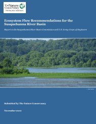
Figure 4.Wanganella Swamps, southern New SouthWales, July 1992Note 3Wetland classificationThe most effective type ofclassification is one that facilitatesthe transfer of scientific knowledgeand management understandingfrom one wetland to another.Aerial photographs, even oblique low-level colour photographs such asthis was originally, are valuable in determining flowpaths during floods,and in revealing impediments. Floodwaters are slightly ponded upstreamof the Cobb Highway. The dominant vegetation is cumbungi, Typhaspp., in the original image looking pink–grey because it is senescent.As with floodplain wetlands (Note 1)this requires a functionalclassification, as done for wetlands inthe Darling system of WesternAustralia (Semeniuk and Semeniuk1995).Most of the wetland classificationscurrently in use in Australia aredescriptive only. Some rely onvegetation presence and abundanceto define wetland types.Unfortunately, this makes it difficultto accommodate change withoutproducing a further classification.Useful discussions of classifications,wetlands and wetland classificationin Australia are given in Pressey andAdam (1995), and in Sainty andJacobs (1994).Evapotranspiration is usually a major component in the water balanceof a floodplain wetland, especially in arid or semi-arid regions.Evapotranspiration depends not only on the local climate — that is, onthe prevailing temperature, humidity and wind speed — but also on thevegetation. Vegetation has a critical role, with species differing intranspiration rates, rooting depth, leaf area, and albedo, a measure ofradiation reflectance. Leaf area also affects direct rainfall interceptionand direct evaporation. The aerodynamic roughness of the vegetationaffects advective interactions with the air above, and this theninfluences transpiration and evaporation. Because of these complexinteracting factors, the accurate determination of evapotranspirationlosses is difficult.On many floodplains, infiltration is directly determined by the durationof flooding, and this determines shallow groundwater recharge. In soilsof low permeability, for example, prolonged flooding is required toachieve significant recharge. Unlike many coastal wetlands or wetlandson sandy soils, groundwater exchange is rarely dominant on floodplainsand it is surface flows, as well as losses via evaporation and plant wateruse, that dominate the water balance.Groundwater losses are difficult to estimate, and although in somecases significant, they are less often a major component of the waterbalance of floodplain wetlands. The importance of groundwaterdepends on the nature of the soils and the underlying aquifers. Coarsealluvial deposits below the contemporary floodplain — that is, thesands and gravels laid down in an earlier phase of floodplaindevelopment — provide aquifers with high water-holding capacity.Such aquifers may be overlaid by fine silts and clays, preventing a directconnection to the surface. These underlying aquifers are an alternativewater source for deep-rooted species such as most floodplain trees andsome shrubs (Section 5, Special studies).When constructing a wetland water balance, a time step must bechosen. The appropriate time step depends on the rate at which14 Estimating the Water Requirements for Plants of Floodplain Wetlands

wetland water levels vary, and the required accuracy of water levelassessment. For small wetlands, or wetlands with frequent or rapidinflows, where fringing vegetation has been identified to be of criticalimportance, levels will vary rapidly and a daily water balance willprobably be required. For larger wetlands, or those with infrequent andslower inflows, a monthly water balance may be sufficient. At each timestep, the water balance calculations will determine the change in waterstorage volume. The time-varying storage volume describes the waterregime of the wetland.Water regimeWater regime is the pattern of water, principally water depth (and thelack of water) through time, so includes duration, seasonality andpredictability. These are considered measures of ‘wetness’ but similarmeasures of ‘dryness’ are equally important for floodplain wetlands indry and hot climates. Dryness can be described, or estimated, bymeasures of soil moisture. The term water regime is used in Australia inpreference to the North American term hydroperiod which is toorestrictive a description with its emphasis on duration and presence ofwater.The water regime of a whole floodplain wetland can be quantitativelydescribed, based on its water balance, as changes in storage volume.Changes in storage can be converted (using a volume-to-arearelationship) to changes in depth. Depth is emphasised here as it is thehydrologic variable of most relevance to most plants. If a wholefloodplain wetland is considered as a single unit, then only an averagedescription of water regime is obtained.Figure 5. Wetland water regimesNote 4Wetland water regimeThis is a list of the preferred wordsand definitions for types of waterregime for Australian wetlands.Williams (1998) recognised threetypes: permanent, intermittent andepisodic, with intermittent andepisodic being separated on thepredictability of flooding. He rejectedtemporary and ephemeral.Paijmans et al. (1985) recognisedfour types: permanent and nearpermanent;seasonal, beingalternately wet and dry; intermittent,meaning alternately but irregularly,wet and dry; and episodic, being drymost of the time.Boulton and Brock (1999) addedephemeral to the list of Paijmans etal. (1985), specifically to includethose wetlands which are floodedvery briefly, perhaps only for days,and unpredictably.Types of wetland water regime are shown here as an interplay of twogradients of increasing ‘wetness’: flood frequency and duration. For clarity,flood frequency is shown as a continuous, qualitative variable, rangingfrom rare to annual flooding, and flood duration as high or low. Floodplainfeatures with high duration are typically cut-off meanders and deflationlakes, all of which are isolated waterbodies, but include also small featuressuch as gilgais and wallows. Areas with low flooding duration are thosewith imperceptible slopes, such as terraces, higher landforms, banks andrelict non-fluvial features.HighEpisodic& lastingNearpermanentPermanentDurationIntermittentNearpermanentLowEphemeralEpisodic& briefEphemeralSeasonalWet – dryRare Low High1:yearFrequencySection 1: Introducing Floodplain Wetlands 15

Floodplain wetlands, being a mosaic of forms (Figures 2 and 3) are alsoa mosaic of water regimes. Flood frequency and duration provide auseful way of describing the range and diversity of water regimes inwetlands, and hence on floodplain wetlands (Figure 5).Note 5Water balance for theGwydir WatercourseThe volume of the GwydirWatercourse (part of the fan-likelower Gwydir River, northern NewSouth Wales) was estimated byBennett and McCosker (1994).Rainfall input was based on averagemonthly rainfall with two states,summer and winter, set at 60 and 35mm per month; evapotranspirationwas based on actual pan records andassumed to be three times as high insummer as in winter, 300 mm and100 mm per month; a target depth of30 cm surface water was chosen asrepresentative of the floodplainwetland area; and water required tofill soil storage was estimated as 30cm under average dry conditions, but50 cm under prolonged dryconditions.A total of 3 ML/ha will be needed ifantecedent conditions are wet, and6 ML/ha if antecedent conditions aredry, with 0.7–2.4 ML/ha per monthto maintain inundation.The interaction of flood frequency and duration accommodates most ofthe terms in common usage. There has been no standard terminology todescribe the different types of wetland water regime (Note 4), althoughthis is beginning to be addressed.Determining the water regime for wetlands and for wetland plants byquantifying wetland water balance is the approach favoured in thisguide. An example, for the Gwydir wetlands, is presented (Note 5).Pathways. A wetland water balance recognises three pathways forwater movement: surface water, sub-surface water and atmosphericwater. Each pathway can move in two directions: inflow and outflowfor surface water; infiltration or re-charge and discharge for sub-surfacewater; and rainfall and evapotranspiration for atmospheric water.Storage volume. At long time scales, the sum of the inputs equals thesum of the outputs, and there is no long-term change in the storagevolume. At shorter time scales, the sum of the inputs does not equal thesum of the outputs, and the storage volume varies considerably.This storage term is the one of most interest here, as it is this term thatdescribes the wetland water regime in terms that link to the floodplainvegetation. The storage volume includes surface water (water above theground surface) and sub-surface water (water stored in the soilcolumn). Sub-surface flow reflects exchanges between the soil storageand deeper aquifers.For large or complex floodplain wetlands, the storage volume can beestimated directly, and approximately, based on inundated area. Forsmall, discrete wetlands where the wetland morphometry is known, orcan be easily established, the storage volume can be determined bymonitoring changes in water levels. Morphometric information is usedto provide a depth–volume relationship. For all wetlands, changes inthe storage can also be calculated from inflow and outflow data. Forthose floodplain wetlands where river flow dominates surface inflow,inputs as run-off and rainfall may be ignored. However, in a fewfloodplain wetlands, notably riverine lakes and floodplains remote fromthe river, direct inputs — whether as rainfall or run-off from the localcatchment — can be significant and may even dominate inflows.Groundwater inflows are typically small on floodplain wetlands,although there may be localised effects on floodplains with lenses ofcoarse material close to the surface. This is not always true forgroundwater outflows.Storage volume hydrographs. Storage volume hydrographs show arecord of the changes in storage volume through time. The shape of astorage volume hydrograph can give a rough idea of which pathway isdominating.Thus, the rising limb (Figure 6) can often be considered asrepresenting only surface inflows. Groundwater inflows can be ignoredduring periods of surface inflow, but may be significant at other times.The effect of groundwater inflows is evident either as a slowing of thefalling limb or as minor rising limbs in their own right, particularly16 Estimating the Water Requirements for Plants of Floodplain Wetlands

when storage volumes are very low. Such inflows will be slow and havea subdued hydrograph peak.The shape of the falling limb (Figure 6) is a combination of surfaceoutflows, evapotranspiration, and groundwater outflow. Becauseevapotranspiration and groundwater outflows are usually slowcompared with surface outflows, the slope of the falling limb indicateswhich outflow pathway is dominant.Figure 6.aStorage volumehydrographsA steep falling limb (Figure 6a) indicates surface-dominated outflows.This can be expected on unconfined floodplains with a surface crosssectionthat is slightly convex, or on higher ground on confinedfloodplains where water returns to the river from the floodplain as riverlevels drop. Terminal wetlands, although often on a floodplain that isconvex overall, usually have depressed areas that retain water and offernear-permanent wet habitat.Slow-falling limbs (Figure 6b) indicate little or no surface outflow, solosses are due to evapotranspiration and groundwater outflow. This canbe expected in billabongs, riverine lakes, and other wetlands onconfined floodplains where surface topography does not allow freesurface drainage.Storage volumebcFalling limbRising limbRapid surface drainage (Figure 6c) occurs after flooding until theminimum level of the outlet channel(s) is reached; further reductions inwater level occur slowly as a result of evapotranspiration and seepage.Section 1: Introducing Floodplain Wetlands 17

Section 2:Introducing theVegetationNote 6Floodplain vegetationGeneral descriptions of wetland andfloodplain plant communities can befound in “The vegetation ofAustralia” (Beadle 1981), in selectedchapters in “Australian vegetation”(Groves 1981, 1994), and there is abrief guide in “Waterplants inAustralia” (Sainty and Jacobs 1994).There is no text dedicated tofloodplain vegetation or its ecology inAustralia but information is includedin “An ecology-flows handbook….”(Young, in press)Note 7Research on floodplainplant ecologyThe ecology of floodplains isdescribed in “Living on thefloodplains” (Mussared 1997).Scientific studies have focused onindividual plant species (usuallystructural dominants) and theirabiotic (usually water, sometimessoil) environment, with only a fewstudies on regeneration anddynamics. “Ecology of fresh waters”(Moss 1998) and “Vegetationprocesses in swamps and floodedplains” (Breen et al. 1988) areamong the few texts that considerfloodplain vegetation.This section gives an ecological background to floodplainvegetation, by looking at some of the ways that water, and waterregime, affect plants. Water is first considered as part of the plantenvironment and described as environmental gradients across thefloodplain, then as a resource, and finally as a resource and asan environment that affects other resources. Vegetation attributesthat are routinely used to describe terrestrial vegetation arepresented, in the context of Australian floodplains. Descriptiveapproaches such as growth-forms and plant functional types areoutlined in relation to the floodplain environment. Plant waterregime and its seven main components are presented, and thevalue of focusing on depth is emphasised.Water as a part of the environmentThe purpose of this section is to introduce floodplain vegetation, firstby describing the spatial character of floodplain as a habitat for plants,and then by giving some background about floodplain plants. Thebackground is necessary because there is no single text on floodplainecology (Notes 6 and 7). Please note that this is not a comprehensiveguide to either plant ecology or floodplains.Wet–dry gradients and patchinessFloodplain wetlands are characterised by having a range of growingconditions: from wet to dry, shallow to deep, favourable to stressful.Which conditions are favourable and which are stressful depends onthe species. This range can be seen as an environmental gradient, from‘wetness’ to ‘dryness’. It is useful to recognise these gradients, not justbecause they determine vegetation patterns but because thisunderstanding can streamline floodplain investigations, especially inrelation to vegetation sampling and water regime.Environmental gradients may be gradients in resources, such asnutrients, or in physical conditions, such as temperature; the gradientscan be described as changes across space, or through time. Anenvironmental gradient need not be water-related, but as this guidefocuses on water management, it is water and water-related gradientsthat are discussed here. On most floodplain wetlands, these are likely tobe the strongest, ie. have the most influence.Examples of spatial gradients occurring on floodplains are:• longitudinal gradient, down the long axis of a river — onconfined floodplains, this is evident as gradual change in flowregime because of progressive flattening and attenuation of the18 Estimating the Water Requirements for Plants of Floodplain Wetlands

flood hydrograph. This corresponds to a gradient in floodfrequency and duration;• lateral gradient, away from the main river channel — onconfined and unconfined floodplains, this corresponds to floodfrequency; this gradient can be broken up by intermediateconditions represented by channels on highly dissectedfloodplains. This corresponds to a gradient in flood frequency andduration;• vertical gradient, for floodplain wetlands with simple forms andespecially around the margins of individual wetlands. Thiscorresponds to a gradient in water depth and duration.These gradients intersect across floodplains (Figure 5). Such gradientsare particularly obvious on infrequently inundated floodplains, wherethe transition from more frequently flooded areas to less frequentlyflooded ones is quite marked. Vertical gradients result in vegetationbanding or zonation around wetlands (Figure 7).Figure 7. Vegetation zonationVegetation zonation showing spatial changes in dominance and structureat Lake Cowal, a floodplain lake in western New South Wales, as it wasin the mid-1970s. The gentle slope at the edge of this shallow lakecorresponds to a flood duration gradient. From the left: The river red gumEucalyptus camaldulensis woodland with scattered river coobah Acaciastenophylla has a well-defined shrub–tussock grass layer, of lignumMuehlenbeckia florulenta and canegrass Eragrostis australasica. Theunderstorey becomes progressively more aquatic, initially with a groundcover of aquatic herbs, mainly nardoo Marsilea drummondi and milfoilMyriophyllum verrucosum, and these are then replaced with beds of thesubmerged herb, Vallisneria sp. Over the same area, as the river redgum trees become less frequent and lose vigour, they are replaced bylignum shrubland, which also eventually becomes sparse. The unevennature of the slope was the result of the construction of farm tanks, damsand channels. Based on Vestjens (1977).On many floodplain wetlands, the pattern of growing conditions ismade more complex by fluvial forms and subtle changes in surfacetopography. For example, on confined or braided floodplains (Figure 3)intersecting channels break the floodplain into patches that may flood atdifferent frequencies, depending on their elevation; and intersectingand diverging channels create flow-paths of variable and changeablevelocity. Floodplains with geomorphic features that retain water, such asbillabongs, depressions, wallows or gilgais, thus have several patcheswhere surface flooding is prolonged.A question of resourcesThe size and vigour of a plant is set by the quantity and availability of theresources needed for growth. Even when these resources are abundant,Section 2: Introducing the Vegetation 19

size and vigour rarely reach their maximum potential because of theeffects of other species, through competition, parasitism and herbivory.In all ecosystems, the quantity, quality and availability of the fourprincipal resources needed by plants — oxygen (O 2 ), carbon dioxide(CO 2 ), light and nutrients — vary. Species have a range of adaptationsto exploit resources when these are available, and strategies toconserve or survive when resources are low or unavailable. Water isessential for plants, as for all living organisms, as it is the medium inwhich biochemical processes take place. For plants, water is needed forphotosynthesis, the process that converts CO 2 into organic compoundsneeded for plant structure, storage and reproduction.More than a resourceConsidering water only as a resource for plants ignores that, for manywetland plants, water has other functions: reservoir, support anddispersal. For submerged plants, or plants with submerged leaves,water is an additional source of nutrients. For many emergent, and mostfloating-leaved species, it offers some support (Figure 8): these plantslack strong supportive tissues so tend to flop when water levels recede.Flood waters help to disperse seeds and other propagules. Species thatare dependent on flooding for dispersal tend to have very buoyantseeds (or fruits); for these plants, the presence of structures such asgates and regulators can adversely affect ecological connectivity.Examples of species with buoyant fruits, but which are not dependenton floodwaters for dispersal, are the introduced burrs, Xanthium spp.The paradox of floodingFlooding creates a paradoxical situation whereby the abundance of oneresource, namely water, alters or reduces the availability of otherresources needed for photosynthesis and growth. This balancing act isillustrated here by focusing on just two of the four main resources —oxygen and carbon dioxide. The fundamental difference betweendryland and wetland plants is that aquatic and amphibious species havea range of physiological and ecological adaptations to compensate fortheir watery environment.OxygenOxygen is freely available in the atmosphere and so to the leaves ofterrestrial plants and to emergent aquatic macrophytes. Oxygen is notfreely available if leaves are submerged.It is a similar story with roots. Roots can respire freely while the soil isaerobic but if the soil is flooded, then soil oxygen is rapidly depleted(by bacterial and plant root respiration) because it is not replenishedfrom the atmosphere. Plant roots become starved of oxygen, andphytotoxins can enter them.Some aquatic plants with aerial leaves have developed ways topressurise oxygen in the leaf and so drive it internally down the plant tothe roots. The capacity to do this is limited to a few growth-forms,mainly emergent and floating-leafed macrophytes. Species with thesegrowth-forms differ in their capacity to pressurise oxygen and toventilate their rhizome and roots, and such differences help explainwhy species differ in their tolerance of different depths of water. Treesapparently do not pressurise oxygen but have developed other20 Estimating the Water Requirements for Plants of Floodplain Wetlands

adaptations. In estuaries, trees such as mangroves have special rootstructures called pneumatophores that project into the air and help toaerate the root system. Some trees such as paperbark and river red gumcan develop adventitious roots in response to flooding. Other trees andshrubs of inland floodplains have few specific adaptations foroxygenating their roots, so their roots are likely to suffer oxygenstarvation under flooding.The time between flooding and when soil oxygen is depleted, and thetime for this to become evident as canopy stress (often yellowing thenleaf senescence), can only ever be an approximate estimate. This isbecause of the influence of sub-surface factors that are difficult to assess,such as how extensive a root system is, presence of air-pockets andmacropores, and soil physical characteristics. Observations forindividual sites are informative and a useful rule-of-thumb but should notbe treated as precise and accurate estimates of flooding tolerance.Carbon dioxideThe availability of inorganic carbon changes after flooding. Carbondioxide is taken up mainly by leaves, through specialised openingscalled stomates. For plants with leaves in the air, CO 2 is freely availableand becomes limiting inside the leaf only if the stomates close, forexample to minimise water loss. The plant must therefore balance takingup carbon and preventing water loss. Because of this, plants in certainenvironments have developed different carbon acquisition strategies,known as C-3, C-4 and CAM (Note 8). The significance of these forunderstanding water requirements of floodplain wetlands, is that C-4plants have a greater water-use efficiency (carbon fixed relative to waterlost) than C-3, but CAM has greater water-use efficiency than C-4.(Section 5, Evapotranspiration).For aquatic plants with submerged leaves, carbon acquisition underwater is a different problem. First, there is the rate of supply. Free CO 2 isavailable to submerged leaves, because CO 2 is very soluble in water, butit diffuses much more slowly than in air, so this can limit plant growth.To compensate for this, some submerged species obtain some of theirCO 2 from the sediment. Second, there is the question of the forms ofcarbon. In water, inorganic carbon is also present in forms other thanCO 2 , and one of these, HCO 3 , can be used by some species. The relativequantities of the forms of inorganic carbon are strongly influenced bypH. Free CO 2 is available only up to pH 7: between pH 7 and pH 10,inorganic carbon is in the form HCO 3 . Thus, long-term or sustainedincreases in pH will disadvantage those species which are obligate CO 2users (Note 8).Note 8Carbon acquisitionstrategiesC-3 is shorthand for plants that fixcarbon dioxide into a three-carbonproduct, and C-4 into a four-carbonproduct. In plants with CAM,‘crassulacean acid metabolism’,carbon dioxide is temporarily fixedas a four-carbon product by nightthen photosynthesis continues duringthe day. C-3 is the most commoncarbon fixing strategy; C-4 is moreprevalent in tropical and subtropicalgrasslands, and in hot, salineconditions, both areas where highwater-use efficiency is an advantage.C-4 plants include some species ofCyperus, Eleocharis, and Paspalum,and some weeds, notablyEchinochloa crus-galli. CAM is theleast common strategy: althoughusually associated with succulentplants, it occurs also in submergedplants from nutrient-poor waters.Information about C-3, C-4 and CAMcan be found in academic texts onplant physiology. The carbonate –bicarbonate – carbon dioxideequilibrium is described in mostaquatic ecology texts, eg. Boultonand Brock (1999); photosynthesis ofsubmerged plants is in Moss (1998).The capacity of Australian submerged plants to use HCO 3 is poorlyknown, although it has been established that Australian material ofCeratophyllum demersum, Potamogeton crispus,Vallisneriaamericana, as well as the introduced Elodea canadensis, can useHCO 3 .Resources without floodingThe dry period between floods creates the opposite resource situation— inadequate water. In warm, dry climates, floodplain plants thatcontinue to grow, albeit slowly between floods, must adapt in some wayto conserve water and to protect against desiccation. Thus, many treesand shrubs from inland floodplains and from episodically floodedSection 2: Introducing the Vegetation 21

floodplains survive there because they have evolved strategies for lowwater use.In contrast, aquatic and wetland plants rarely have water-conservingstrategies. Submerged plants, for example, have leaves rarely more thana few cells thick and virtually no protective outer cuticle, so theydehydrate rapidly in the sun. Wetland plants with aerial leaves, such asemergent and floating-leafed macrophytes, have a thick or waxy cuticleon their leaves but transpire readily.Most aquatic plants ‘ride out’ the dry inter-flood periods by strategiesother than physiological adaptations. One strategy that is typical ofannuals is avoidance, exemplified by short life-span and setting seeds,hence reliance on the seed-bank. Another strategy, typical of perennials,is to enter a low-activity or no-growth phase. In this, water loss isrestricted by leaf-shedding, or by complete canopy senescence and dieback.The plant survives with its sensitive generative tissues buried inthe sediment, or as hard-coated seeds or some other propagules.Aquatic plants have a wider range of propagules than do terrestrialspecies, with rhizomes, corms, tubers, turions, spores and nodalfragments as well as seeds.The long-term survival of these propagules depends on being buried inprotective sediments and on the sediments being protected fromdisintegration by trampling or machinery. In general, water-conservingstrategies are better developed in shrub and tree species occurring onthe infrequently-flooded parts of floodplains.Adaptations, tolerance and stressDifferences in adaptation to resource availability means species arefound in particular sequences, ie. at different positions on theenvironmental gradient from ‘flooded’ to ‘dry’. This is evident inzonation (Figure 7), the concentric patterns of species in the littoralzone around a billabong or up a riverbank. On a larger scale, a similardistribution can be seen across a floodplain.The degree of adaptation can be described as obligate or facultative;and adapted or tolerant. In the floodplain wetland context, speciesdependent on aquatic conditions to provide resources, support andopportunity for regeneration are obligate species, whereas those thatcan survive on wet muds (at least temporarily) after flood recession andstill flower and set seed, are facultative. Thus, submerged plants such asVallisneria which die of desiccation on flood recession are obligate forinundation, whereas many species of milfoil, Myriophyllum spp., thatcan grow on wet muds, especially during cooler conditions, arefacultative. Similarly, species may be flood-adapted, meaning they havespecific adaptations that allow growth under flooded conditions,whereas species that survive but are not adapted to grow are floodtolerant.An equivalent situation occurs in relation to dry conditions onthe higher parts of a floodplain, where plants may be drought-adaptedor drought-tolerant.The tolerance range of a species to a particular component of the waterregime, such as depth, can be inferred in various ways, includingspecific investigations. Descriptive generalisations such as growth-formcan be helpful (Figure 8).22 Estimating the Water Requirements for Plants of Floodplain Wetlands

Floodplain vegetationEcological rangeThe array of plants on floodplains includes species that are adapted todry, almost terrestrial, conditions, to aquatic conditions, and to thevarious intermediate conditions. Words used in this guide to refer tothese plants are given below:Aquatic plants usually refers to those plants that are adapted togrowing in, on or under water. Definitions vary, and while it is easy toagree that submerged species are aquatics, it is not always accepted thatmedium–tall sedges such as Eleocharis acuta and E. dulcis fromintermittent or seasonal wetlands are aquatics. Aquatic plants may alsobe known as water plants, or hydrophytes.Amphibious plants are those plants that grow or survive on wetexposed mud flats. These may be aquatic plants such as Ludwigiapeploides, stranded by falling water levels, or a completely differenttype of plant, the semi-terrestrial ones that germinate and grow rapidlyin these conditions (Figure 9).Wetland plants are those found growing in a wetland. In wet–dryfloodplains, they include amphibious and terrestrial and, arguably, alsoexotic species. The definition of wetland plants is probably the leastprecise of the definitions listed here.Macrophyte means literally ‘large plant’, a name coined originally todistinguish these from microphytes such as phytoplankton. It is nowused almost interchangeably with aquatic plants, and includes thestoneworts Chara and Nitella in the family Characeae because, eventhough these are algae, they have a herb-like form.These terms, being difficult to define satisfactorily for all conditions andall plants, are flexible. When buying or using books to identify wetlandand floodplain or aquatic plants, it is advisable to check the definitionsbeing used. Only State or national floras are fully comprehensive.The plants may be short- or long-lived perennials, biennials or shortlivedannuals; they may be small or simple forms, such as duckweedsand charophytes, or large woody species, such as trees.Temporal changesOn wet–dry floodplains, the changes that result from flooding and laterfrom flood recession, provide a brief but distinct growing opportunity.Short-lived and dormant herbs and forbs, that is herbaceous plants otherthan grasses, grow quickly; rapid growth alters the appearance of aperennial community.A lignum shrubland may have an understorey of short sedges, aquaticherbs or terrestrial grasses, depending on time since flooding, but is stilla lignum shrubland. If, however, the lignum is removed, then what wasthe understorey now appears as a dynamic, constantly changingwetland plant community.It would be a mistake to interpret all herb–forb wetland plantcommunities as the result of disturbance. The aquatic herbs thatgerminate or regrow on lagoon floors after flooding are a transient plantcommunity; as the wetland dries out, the plants in this community die.Section 2: Introducing the Vegetation 23

The lagoon floor is then colonised by opportunistic, amphibious thenterrestrial species, and the previous community persists as propagulesand seeds.Note 9Vegetation structure ashabitatPlants are habitat that is exploited bydifferent species, for different lengthsof time, and for different reasons.The undersides of floating leaves maybe grazed daily by molluscs; beds ofsubmerged plants may becomenursery areas for weeks; denseriparian shrubs may periodicallybecome a velocity shelter for fishduring floods; emergentmacrophytes or lignum may benesting sites in most years. The valueof plants as habitat is contingent onthe environment. For example, astudy of darters, cormorants, heronsand egrets on the MurrumbidgeeRiver found that although these allnested in river red gums Eucalyptuscamaldulensis, species differed inthe type of tree chosen, and in howmany species ‘shared’ a tree. Unlikeother waterbirds, great cormorantsnested in dead trees, probablybecause these were associated with anear-permanent water regime(Briggs et al. 1993). Considerationof vegetation as habitat needs toinclude not just living plants, butdead ones such as debris dams andsnags.Structural diversityThe structure of a plant community is its three-dimensionalorganisation. Terms to describe vegetation structure come from bothterrestrial and aquatic plant ecology, and both are necessary to describethe vegetation of floodplain wetlands. Simplistically, structure meansthe height, density and species composition for each vegetation layer.Typical terrestrial growth-forms are trees, shrubs and tussock grasses.These give rise to vegetation types such as forests and woodlands,shrublands and perennial grasslands. Their vertical structure is veryevident, being at the scale of the human observer.Typical aquatic growth-forms are emergent macrophytes, whichcomprise mainly grasses, sedges and rushes; submerged macrophytes;floating-leafed plants and free-floating plants. These form distinctivegrasslands, sedgelands and herblands. Their structure may be partlyunderwater, and is generally much less obvious to the human observer.The range of structural vegetation types on a given floodplain isdetermined by its ecological diversity and by its location, whethertropical or temperate, coastal or inland. Vegetation structure issignificant because it determines habitat for floodplain fauna, bothabove and below the water. Fauna respond to different vegetationattributes, depending on animal size and need (Note 9). Some speciescan be quite narrow in their requirements, which need to be carefullyincluded. Structural diversity is high across floodplains because of thediversity of the plant communities, but is lower within each plantcommunity.Distribution of floodplain speciesMany floodplain species have a fairly wide geographic range and sooccur on more than one floodplain, but within a climatic range.Examples of species with a wide geographic range are river red gumEucalyptus camaldulensis, and lignum Muehlenbeckia florulenta.Species composition of a floodplain is therefore not unique. Instead,there is considerable overlap between floodplains, especially thosewhich are close or have similar soils and climate, or are in sameecoregion, or ecological region. An Australia-wide system ofbiogeographic regions has been developed. It is known as the InterimBiogeographic Regionalisation of Australia (see Web Listings section)and is the best guide presently available.Some species have a restricted range or are confined to just onefloodplain or catchment. An example of a floodplain tree with limiteddistribution is yapunyah Eucalyptus ochrophloia, which is found innorth-western New South Wales and south-western Queensland (Note10).Wide geographic range is characteristic of many aquatic and wetlandplants. Some occur across ecoregions, showing a temperature tolerance.Some are found across the Australian continent, such as Typhadomingensis, which is naturally widespread, and Typha orientalis,which has a distribution that has been extended westwards across thecontinent since European settlement. A few native aquatic and wetland24 Estimating the Water Requirements for Plants of Floodplain Wetlands

species have an even wider geographic range. Species such asPhragmites australis,Azolla filiculoides,Potamogeton crispus andPaspalum distichum are found in both Northern and SouthernHemispheres: plants such as these with very wide distributions are calledcosmopolitan. Many Australian aquatic and wetland species belong togenera that are widespread across Australia, and across the world. Theyinclude Potamogeton,Eleocharis,Cyperus, and Myriophyllum.Species richness — the number of species per hectare of floodplain —is not particularly high on inland warm–temperate floodplains,especially when compared with wet heathlands or some terrestrialplant communities in Australia. Inland floodplains typically record100–200 plant species overall. Species richness is apparently muchhigher in other floodplains, such as coastal floodplains of northern NewSouth Wales where 70–100 aquatic macrophyte species alone have beenrecorded, and tropical floodplains where 200–300 species have beenrecorded. Species richness is much higher in disturbed and developedcatchments, where it is boosted by non-native species, mostlyagricultural weeds or escapees: these may be as much as20–30% of the total species count.DescriptionThe formal description of plant communities should include some detailon floristics, structure, abundance and even comments on vigour. Todate it has been a common practice to refer to floodplain communitiesin a short-hand form, by their dominant species and its growth-form; forexample, lignum shrublands, black box woodlands, red gum forests,cane grass grasslands.These ‘species + growth-form’ descriptions are useful but limited:‘species + growth-form’ is an incomplete description of a plantcommunity, as it gives no information on species other than thedominant one and little information on structure.Note 10Biogeography of waterplantsFor water plants, the greatest floristicdifferences across Australia arebetween temperate and tropicalregions. This is true at the level ofspecies, genus and family. In a givenregion, there are nearly twice asmany monocot species as dicotspecies, 50–70% compared with24–41%; ferns are usually poorlyrepresented with only about 5% of allwaterplant species. Endemism, thatis the number of species restricted toa region, is generally low in southeasternand temperate Australia(1–5% of waterplant species), ismarginally higher in tropical regions(approximately 8%). Endemism isquite significant in the south-west ofWestern Australia and in NewZealand (38–44%). For more, seeoriginal scientific paper by Jacobsand Wilson (1995).Ecological groupsEcological groups are a means of reducing bulky amounts of informationabout species. Such groups, even if they are only approximate and arebased on incomplete science, can still serve, to a limited extent, as arough ‘model’ (a guide to) of species behaviour or response. Ecologicalgroups can be based on observations, assumptions, or measurements,and are typically a mixture of all three. Two types of ecological groupsrelevant to water management and to understanding wetland plants aregrowth-forms and plant functional types, or PFTs.Aquatic growth-formsSome understanding of how well plants are adapted to aquaticconditions can be inferred from their growth-form.Plants with comparable morphology, or shape, are said to have the samegrowth-form. For aquatic and wetland plants, growth-form indicates,very roughly, the position of roots and leaves relative to water level, andto sediment. Growth-form is therefore a useful first approximation ofadaptation to the aquatic environment and, being based on visualinformation, is easy to apply (Note 11).Section 2: Introducing the Vegetation 25

Note 11Growth-formsField guides to wetland plantsemphasise visual cues, so tend to usegrowth-form as part of the identifyingcharacteristics. Growth-form isusually combined with othercharacteristics, often expressed inplain English; for example, growthformand leaf shape “submerged, notfeathery” is used by Sainty andJacobs (1994). See Hutchinson(1975) for an introduction tohistorical terminology and thesource of technical words such ashydrophytes and macrophytes.However, growth-form does not make perfect predictions about how agroup of species responds to water regime. This is because growth-formis not a complete summary of all adaptations, nor do all species withthe same growth-form have the same adaptations. Growth-form refersto only one phase in the life cycle, the established adult, and to just onepart of a plant’s environment, namely water level. Conventionaldescriptions of growth-form do not cover amphibious or mudflatspecies very well.Figure 8. Structural diversityIn wet seasons, floodwaters spread into rarely-flooded areas where thespecies of macrophytes that develop are influenced by the season offlooding. Autumn flooding on the Murrumbidgee floodplain hasproduced a sparse cover of Marsilea drummondii, Triglochin dubium,Rumex and unidentified grasses. Nearby (not shown) was densecontinuous growth of Eleocharis acuta in shallow ponded water; indeeper water, dense beds of Characeae and Damasonium minus withabundant shield shrimps, Notostraca. Delta Creek, May 1990.For a description of terrestrialgrowth-forms current in Australia,see Walker and Hopkins (1990).Although widely used in scientific and general literature, there is nostandard set of names for growth-forms. This is not as frustrating as itsounds, because modern practice is to use descriptions such as freefloatingor floating-leafed plant, rather than classical terminology (Note11). In the past, scientists struggled to develop an all-encompassing setof names to describe all aquatic and some amphibious growth-forms.This resulted in a plethora of quasi-technical terms in the scientificliterature of up to about 25 years ago. A few, such as hydrophyte andmacrophyte, remain current. A limited number of conventional aquaticgrowth-forms is used in this guide (Figure 9).Plant functional typesPlant functional types (PFT) are groups of plants with a similar responseor responses to one or a range of specific environmental conditions,such as resource availability or disturbance. Responses are a set of traits.The traits may be measurements, such as biomass, seed size or specificleaf area, or may be based on published knowledge, such as whether aplant is a C-3 or a C-4 species. The choice of these traits assumes theyare representative of, or correlate with, ecological characteristics suchas competitiveness, seedbank longevity or relative growth rate.Alternatively, traits may be empirically defined through experiments;for example, by germinating or growing a number of species under26 Estimating the Water Requirements for Plants of Floodplain Wetlands

Figure 9. Aquatic growth-formsText gives a general description, with notes on adaptations and some examples. Diagrams are drawn to differentscales, (*) indicates an introduced species.EMERGENT MACROPHYTES – erect formsRooted in sediment, leaves growing through water, into air. Size ranges from tall >1 m, medium to small. C-3 and C-4species. Forms with leaf blades have high surface area, often very productive. Tall forms often dominant.Can grow in permanent water, but tolerant of periodic temporary dry conditions or deeper water. Rhizome and rhizosphereoxygenated from leaves.Tall and medium forms are mainly perennials. Most perennials have substantial underground carbohydrate storage, usuallyrhizomes but sometimes as corms or tubers.Monocots, mostly from Cyperaceae or Poaceae. Examples of species are Typha, Phragmites, Eleocharis, Cyperus, Baumea,Bolboschoenus, Juncus.EMERGENT MACROPHYTES – trailing formsRooted at channel edge or bank. Leaves on water or slightly rising above surface, from floating stems or stolons. Traildownstream in low-velocity current.Buoyancy mechanisms for stems not always evident but can include inflated hollow stems, spongy tissues. Stems flexible,not rigid, so move easily with small changes in water level or waves.Many species have rootlets at nodes, some species can establish from fragments with these.Examples: Ludwigia peploides, Rumex bidens (*), Nymphoides spp., also several grasses with prostrate-ascending stems,eg. Pseudoraphis spinescens.FLOATING-LEAFED MACROPHYTES – trailing formsRooted in sediment, leaves floating on water surface. Floating leaf typically rounded or oval, glossy above, and may becomemore erect when leaves are crowded. Some species have, initially, submerged leaves.Grow in or near permanent water, to 2 m sometimes 3 m, depth range defined by length of stem or petiole. Stems havelacunae, and/or aerenchyma, to facilitate internal movement of gases.Mainly perennials. Rhizome may be compact at stem base, or bulky and extensive.Species in the family Nymphaceae, also Ottelia ovalifolia, Brasenia schreberi, Potamogeton tricarinatus, Marsilea spp.,Villarsia reniformis, Nelumbo nucifera.SUBMERGED MACROPHYTERooted in sediment, and grow submerged in water,

identical conditions. PFTs differ from growth-form in that they focus onassumed or observed responses.PFTs can be used in models of vegetation change. This is an attractiveapproach because it is a way of reducing the enormous complexity ofmodelling species individually to a few recurrent patterns. PFTs haveyet to be used in modelling dynamics of floodplain vegetation. This willrequire putting species into functional groups based on their responsesto flooding and drying, and to changes in water regime. The system ofPFTs developed for wetland plants (Figure 10 and Note 12) is relevant,at least to part of floodplain wetlands; no PFTs have yet been workedout that include both floodplain and wetland species.Figure 10. Wetland plant functional typesSeven plant functional types identified from 60 wetland plant species, onlagoons on the New England Tablelands (diagram supplied byM. Brock, 1999).WETLAND PLANTSresponse to water presence or absenceTerrestrialDoes not tolerate floodingAmphibiousTolerates flooding and dryingSubmergedDoes not tolerate dryingAmphibious:Fluctuation-toleratorsAmphibious:Fluctuation-respondersTerrestriale.g. Cirsium sp.emergent vines low growing treese.g. Eleocharis spp.e.g. Hydrocotyle sp.morphologicallyplastice.g. Myriophyllum sp.floatinge.g.Nymphoides sp.Submergede.g. Vallisneria sp.Plant water regimeThe water regime of a floodplain wetland is its characteristic pattern offlooding, drying or water-level changes. These changes can bedescribed in terms of when water level changes occur, how much, howfast and for how long (Figure 5). For plants, water regime is also thepattern of flooding, drying or water-level changes but it refers to thespecific patterns needed to ensure species maintenance andregeneration.• A maintenance water regime, as used here, is the water regimeneeded by an established mature plant to survive in the long-term;that is to grow and to periodically flower, and also to set seed atintervals that ensure the population seedbank or propagule bankis maintained.28 Estimating the Water Requirements for Plants of Floodplain Wetlands

• A regeneration water regime is one that ensures periodicestablishment or re-establishment of plants, whether from seed orfrom other propagules. If from seed, then the regeneration waterregime must satisfy conditions for seed germination followed bysuccessful seedling establishment; if from propagules, then thereare similar requirements for initial or follow-on conditions,although these may be subtly different.Maintenance and regeneration requirements are usually quite different.The environmental conditions required for germination, or for survivalof a seedling, are not the same as those required by the adult plant. Forexample, many emergent macrophytes germinate on wet muds,comparable to drawdown conditions; only some have seedlings that cantolerate submergence. Shallow water is likely to be detrimental, at leastuntil the plant reaches a critical stage: in contrast, adult plants cantolerate water depths ranging from 0 to about 1.5 metres.Components of plant water regimeWater regime refers to the hydrograph shape and size, and the patternof hydrographs through time. Size and shape characteristics arecorrelated under natural conditions, but this can change once a river isregulated or its flow regime modified. Describing a hydrograph shapeand the pattern of hydrographs through time in terms of its componentsis useful, in terms of clarifying plant responses. Seven components canbe recognised (see below): of these, the most frequently studied aredepth and frequency.Depth: The importance of depth and the effects of changing depth arevery much dependent on species growth-form and size. Plants withrigid or erect aerial leaves, such as emergent macrophytes, seedlings andtussock grasses, can grow in water to a certain depth, depending ontheir height or size. Equally, they can tolerate an increase in waterdepth, provided a reasonable proportion of the canopy or stem is notsubmerged, otherwise they become stressed or may even die (Note 13).Thus, although depth is measured in absolute terms, in millimetres ormetres, the ecological effect on these plants depends on the size of thespecies in question. Floating-leafed plants with flexible petioles cangrow in water up to two metres deep, depending on how effectively therhizome is ventilated from the leaf, and can tolerate fluctuations inwater level, roughly of 10–20 cm, such as caused by wind-inducedwaves. Free-floating and submerged forms are not greatly affected byincreases in depth, unless this causes a reduction in light.Note 12PFTs on TablelandlagoonsThe first Australian study of wetlandPFTs was done on isolated lagoonson the New England Tablelands.Seven PFTs were defined in terms oftheir response to water regime(Brock and Casanova 1997).These seven PFTs were empiricallydetermined by a combination ofexperiment and observation of 60wetland plants. The lagoons havevariable water levels and anintermittent water regime, and thelittoral zone, being periodicallyexposed and submerged, meansthese lagoons are a variable andunpredictable environment in whichto grow and the complete plant lifecycle.Several of the 60 species used in thisstudy are also found on inlandfloodplains, but dominant floodplainspecies are not included.An alternative system of wetland PFTshas been developed in North Americabut not yet applied in Australia. Thisrecognises three main plant types:ruderal, matrix, and interstitial: it isuseful for disturbance rather thanwater regime (Boutin and Keddy1993).Duration of inundation: Duration refers to the time that surfacewater is present, measured in weeks or months. Duration is importantfor obligate aquatics as it defines the potential growing period for adults,including flowering and seed-set or storage, or the time frame forgermination and seed-set if an annual. For facultative aquatics or thosetolerant of mud-flats, conditions may be favourable for growth even afterthere is no more surface water, for as long as the soils remainwaterlogged or moist. For floodplain species, duration of floodingdefines the period when soil water is recharged by infiltration.Season of flooding: Season, or timing, here refers to when floodingbegins. Season is significant because it is a short-hand way to refer to acombination of climatic factors that affects plants: temperature, daylength,and whether day-length is increasing or decreasing. Temperaturedetermines the rate of physiological processes, evident as growth;Section 2: Introducing the Vegetation 29

Note 13Changes in depthSome herbaceous non-woodyspecies with aerial leaves show asurprisingly quick response toincreases in water depth. The stemcarrying the leaf, or the leaf itself,grows rapidly to the surface. Forexample, the rhizomatous fern,Marsilea mutica, can grow through10 cm water to reach the airovernight, and through 100 cm inabout 6 days (Yen and Myerscough1989).Response to increased depth tends tobe slower in emergent macrophytessuch as Baumea arthrophylla,Bolboschoenus medianus, andTypha orientalis, and for these,increases in depth typically result ina change in resource allocation,indicated by how much of plantbiomass is root, rhizome and canopy.This represents a shift in theimportance of nutrient uptake,storage and photosynthesis, andhence a shift in growth strategy (eg.Rae and Ganf 1994, Froend andMcComb 1994, Blanch et al. 1999).Amphibious plants, such as themilfoil Myriophyllum variifolium,have developed morphologicalplasticity for the wet–dry littoral zone(Brock 1991, Casanova and Brock1991).temperature can limit germination, as some species have germinationtemperature thresholds. Day-length determines the energy available forphotosynthesis. Some species have specific day-length and/ortemperature requirements or tolerances, and may be winter-growers orsummer-growers. For long-lived woody species, such as riparian trees(eg. black box Eucalyptus largiflorens) season of flooding may be moreimportant for flowering than for leaf growth. Responses to climate is aspecies-specific response, and is not linked to growth-form, as theexample for two emergent macrophytes shows (Note 14).Rate of rise: Rapid increases in water-level may submerge emergentand floating-leafed aquatic plants unless they can grow or extend fastenough to keep the leaf or the photosynthetic stem, known as a culm,in the aerial environment (Note 13).Frequency: Frequency is the number of times flooding occurs. Annualand short-lived aquatic plants (ie. those living for less than one year) aregenerally flooded only once in a life-span; perennial aquatic and woodyfloodplain species may be flooded several times, ranging from once oreven twice per year to once every five to seven years, or even lessoften. For these, frequency is a long-term average (which does notaccount for variability). Flooding can be the stimulus or opportunity toflower and set seed; thus flooding at a critical frequency is essential forspecies dependent on the seedbank to maintain their presence. In theabsence of flooding, a seedbank ages and propagules lose viability. Forperennials, flooding is typically the time when resource constraints arelifted: plants can replenish their reserves, flower and so recharge theseedbank. Frequency thus influences population long-term vigour andhence survival.Inter-flood interval: The inter-flood interval is the period withoutflooding. The length and recurrence of this is most relevant to thoseplants that maintain a low level of growth in the absence of flooding,such as perennials on the higher and drier parts of floodplains. Here,the inter-flood interval can be a period of water stress, so its durationand recurrence and timing will affect long-term vigour. Perennialspecies survive this period through water-conserving mechanisms. Oninland floodplains, trees (and possibly shrubs, though this has not beendetermined) are opportunistic water-users, and can utilise other watersources, such as heavy rainstorms and groundwater, if and when theseare available.Variability: Variability refers to the regularity or range of values for anyof the components of water regime, although is more usually reservedfor flood frequency.Important componentsThe relative importance of these seven components for a particularplant species or group of species has not been determined, and wouldrequire a complex experiment to disentangle. As a rule of thumb, it issuggested that depth, duration, and season are most important at anannual time scale, but that frequency, inter-flood interval and variability(or its converse, regularity) are most important over longer time-scales.Unlike in rivers, velocity is not an important component of the waterregime for plants of floodplain wetlands. This is because velocity onfloodplains, consistent with their being depositional areas, is generallymuch slower than in the main river channel, even during floods. In-30 Estimating the Water Requirements for Plants of Floodplain Wetlands

channel habitat does occur on some floodplains, and these flowpathsmay have a fringe of emergent and trailing plants on their banks. Highvelocity channels may acquire characteristics and species more typicalof river channels.Although it is not an important component of water regime for plants,velocity is nonetheless significant on the floodplain, especially thosefloodplains that have been cleared or where channel bed has degraded,ie. become cut down, as the result of channel erosion. For these, therelationship between flow and inundated area (Section 6 and Figure 23)has changed. Flowpaths are generally only a small fraction of afloodplain wetland, usually too small to be recognised within a wholefloodplain management plan, except by hydraulic modelling.The effects of changing water regimeThe effect on the vegetation of changing one or more components in awater regime depends on which components are altered, and whatspecies are present.If water regime changes from intermittent to near permanent (Figure 5),the increase in flood frequency or flood duration means soils may notreturn to their earlier aerobic condition, resulting in soil waterloggingand deoxygenation. This is an opportunity for invasive plants tolerant ofwetter conditions, or for plants requiring a wet sequence to germinateand establish. However, these conditions cause stress or even death forperennial species reliant on soil oxygen.If an area is flooded less often and/or for shorter periods, ie. the waterregime changes from seasonal to intermittent (Figure 5), then soils willtend to dry out. This will result in widespread water stress or localiseddeath of perennial floodplain plants that are intolerant of drought or notadapted to dry conditions, and the expansion of terrestrial annuals andother opportunistic species.If season of flooding changes from winter to summer, as on manyregulated rivers, then a species shift to summer-growers can beexpected.The consequences of increasing or decreasing one or two componentscan be anticipated from the frequency–duration grouping of waterregimes (Figure 5). Shifting from near permanent to permanent is less ofan ecological change than shifting from episodic brief to nearpermanent, although a change nonetheless. Changing the season offlooding or of draw-down is not covered in the frequency–durationdiagram, but can be expected to lead to a major change on plantspecies.Note 14SeasonalityThe ecological consequences ofchanging seasonal patterns in flowregime have not received as muchattention as, for example, floodingfrequency.Not only can changes in seasonalitylead to changes in speciescomposition, but to structuralchanges. For example, native aquaticgrasslands are being invaded by thedominant tree species in the BarmahForest (Bren 1992) as a result ofseasonal changes.Species seasonal responses, whetherfor maintenance or regeneration,cannot be anticipated fromecological types such as growthformsor PFTs, so must bedetermined from the literature orthrough special studies. Forexample, contemporary studies oftwo emergent macrophytes done inthe same locality found that, forTypha orientalis, the main period ofcanopy development was August toDecember with biomass peaking inDecember–January, whereas forPhragmites australis, it was spring–summer, August to March withbiomass peaking in March–April,(Hocking 1989, Roberts and Ganf1986).For an experimental study of theimportance of season of flooding, seeNielsen and Chick (1997) andBritton and Brock (1994) onseedbanks.Changes which cause a loss of vigour in one species may favour another.Such a change can be an opportunity for exotic species to establish. Ifexotic species are the focus of a water management plan, it will benecessary to establish that water regime is the sole factor contributingto its establishment and persistence. Establishment may be encouragedby repeated disturbance, such as cattle trampling, or by preferentialgrazing, and persistence may be the result of a long-lived seedbank.Restoring an original water regime is not a guaranteethat the exotic plant species will disappear.Section 2: Introducing the Vegetation 31

Focusing on depthWater regime analysis needs to consider all components of plant waterregime. A limitation of most field investigations is their emphasis on justone, sometimes two, components, with the assumption that othercomponents have not changed. Flood frequency is often chosen,probably because it is easily quantified by inundation mapping andhydrologic modelling, but it is only one of seven components.With floodplain wetlands, the sheer size and diversity of the floodplainarea presents particular challenges. Unlike small, isolated waterbodieswhere frequency, magnitude and duration of flooding are relativelyuniform or tightly correlated, water regime is not uniform across thefloodplain; thus, statistics based on spatial averages may not bemeaningful. Ideally, flood frequency and duration, and othercomponents of plant water regime, should be estimated forhydrologically homogeneous sub-units of the floodplain wetland.However, this could result in working with numerous, very smallmanagement sub-units, making modelling an impossibility. Typically,these sub-units are aggregated and larger spatial units such as plantcommunities are considered.An alternative is to reinterpret plant water regime as spatial andtemporal variations of just one component — depth — by workingwith three states:• inundated and submerged;• inundated, but not submerged; and• not inundated.In this way, plant water regime can be modelled as a time series of thesethree states. For each state, key statistics are the mean duration and thevariability of the duration. Other useful statistics are the mean andvariability of the period between the occurrence of a given state, andthe seasonal occurrence of the three different states.Focusing on depth represents an ideal, targeted at developing models.Even if modelling is not the aim, focusing on depth is one way toreduce complexity and make it easier to work with water regime.32 Estimating the Water Requirements for Plants of Floodplain Wetlands

Section 3: A StepwiseProcedureThe process for determining the water requirements for plants offloodplain wetlands can appear complicated and even circular tothose involved in the process, but in fact it follows a series of welldefinedsteps. These steps are similar regardless of politicalprocess or which floodplain wetland is being considered. Thissection describes the five steps in this general procedure. OnlySteps 3 and 4, both purely biophysical, are treated in detail here.OutlineThe general procedure comprises five steps (Figure 11) which shouldbe followed in every investigation.Figure 11. Flow chart showing five steps for determiningthe water requirements of floodplain wetlandsplants5aRefine vegetationmanagementobjectives?ImplementationAcceptable balance?5Trade-off process with otherwater uses4Determine water regime to achievemanagement objectives3aImproverelationshipsto generatenew ones?Relationship definitions OK?3Describe relationships betweenvegetation & water regime2Set vegetation relatedmanagement objectives1Describe ecology, hydrology,uses & valuesSection 3: A Step-wise Procedure 33

Note 15Internet dataEnvironmental data are availablefrom Internet sites such as LongPaddock and Bureau of Meteorologyfor weather records, Bureau of RuralScience for soil maps — particularlyin the Murray–Darling Basin, andAUSLIG for satellite imagery. Fulldetails are given in the Web Listings.Note 16Historical dataHistorical information can have aspecial role. It is an opportunity forinterested individuals or groups tocontribute. However, historicalinformation is generally sparse,difficult to find, rarely quantitativeand sometimes of doubtful technicalquality. Because of this, historicalprojects may need differentmanagement and clear goals.Historical studies may contribute inthree ways.One: as data, contributinginformation and helping to fill gapsin the scientific record. This canextend understanding beyond what isknown by the investigators. Anexample is compiling past floodhistories, as done on the DarlingAnabranch (Withers 1994).Two: an understanding of what hashappened, especially in terms of pastland uses, can help explain someenvironmental and vegetationpatchiness and anomalies. This willaffect sampling design, improving itand interpretation.Three: in highly modified floodplainwetlands, knowing the past conditioncan help clarify management goals,as happened at the Moira Lakes andon parts of the Lachlan River(Roberts and Sainty, in press).The data, tools and techniques used in each step will vary from onefloodplain plan to another, depending on circumstances such asopportunities and constraints. For example, time and resourceconstraints will vary between investigations, as will the extent andusefulness of existing data.This general procedure makes only two assumptions: one, that themanagement objectives relate in some way to the vegetation, whether itis abundance, character or condition; and two, that these measures ofvegetation (abundance, character and condition) are dependent tosome degree on the water regime of the floodplain wetland. The degreeto which this dependency — or relationship — is describable will vary.Thus, the main variations in the general procedure are in the tools andtechniques used in acquiring and analysing vegetation and waterregime data (Step 3), and in the tools and techniques used in predictingvegetation response to water regime changes (Step 4).It is these twosteps that this guide addresses.Step 1: Describing the floodplain wetland1The first step is to describe the floodplain wetland using onlyavailable data and information.‘Description’ here means the floodplain wetland’s water balance, itsecology, especially as this relates to floodplain vegetation, and its usesand values. These data will be in a range of formats — as reports, aselectronic data, as maps and on the Web (Note 15). Collection of newdata may be required later in the process, once management objectivesare made clear, and once gaps in knowledge gaps have been identified.Information on the most important component of plant–water regime,the spatial and temporal variation in water depth, is rarely available or isquite limited. At this stage, description is likely to focus on the waterbalance of the floodplain wetland. Information useful for describing allsix components of the water balance is described above (Section 1):local climate, surface and groundwater flow, and plant water-use orevapotranspiration data. In addition, information on wetland soils can beof use in quantifying the water regime. Typically, however, the hydrologydata that are directly available will be limited to, for example, relativelyshort records for one or two components, or to particular flood events.Information useful for describing floodplain wetland vegetationincludes vegetation or land-use maps, aerial photographs and satelliteimages. Historical information has a particular role (Note 16) and maybe useful in describing species response and changes in plantcommunities. The value of historical information depends on knowingits context, ie. its date and location, so that the contemporary weatherand/or flooding conditions can be established, and its locality. Detailedinformation, such as vegetation transects, ground cover andunderstorey species in forest and woodland areas, may be availablefrom agency or station records; although this can be extremely useful, itis seldom available at the start of an investigation. Vegetation data areusually patchy, and maps are scarce, and may be out of date. Despitethese drawbacks, what is available may be adequate to set managementgoals, as in Step 2. Most of what is needed in Steps 3 will have to bespecifically collected.34 Estimating the Water Requirements for Plants of Floodplain Wetlands

All the uses and values that relate in some way to the vegetation of thefloodplain wetland must be identified: conservation, environmentalprotection, grazing, recreation, and tourism. These uses and values maybe linked to specific types of land tenure, whether private or public.Conservation values may be associated with the protection ofendangered or threatened species, or with certain features of thevegetation for habitat. Recreation may be water-based (for example,canoeing) or nature-based, such as bird watching. Grazing may beassociated with one particular plant community or even species.Collating such information will provide an understanding of thecharacter, function and values of the floodplain wetland underconsideration.Step 2: Setting management objectives2The second step is to set the management objectives specific tofloodplain vegetation.Early in an investigation a statement of the vegetation-relatedmanagement objectives must be attempted. These will be a sub-set ofthe complete set of management objectives. They are not limited to theenvironmental objectives, but include objectives relating to anyproductive or economic uses that depend on the vegetation or itscondition, eg. floodplain grazing and honey or timber production (Note17).These objectives should be stated as quantitatively as possible. This canbe done by identifying appropriate vegetation measures, and settingtarget values for these measures. Abundance, character, and condition ofvegetation must be related to wetland water regime (Step 3). Examplesof such measures are the area of each plant community, specific mix ofplant community types (eg. grassland, shrubland, and woodland),species diversity in different plant communities, balance of native andintroduced species, and the condition of a particular community orspecies. Surrogate measures may also be useful: these are measureswhich provide an indirect indication of the attribute of interest. Anexample of a surrogate measure is using the condition of a species toindicate the condition of an entire plant community. To be useful in anongoing management sense, all measures need to be amenable tomonitoring, so it is possible to assess how well management objectivesare being met.Note 17Setting targetsWater regime targets can be set quitesimply, as in a restoration program:return the water regime to itsoriginal condition, or as close aspossible. Other vegetation targets canbe set, through a communityconsultative process, and the waterregime needed to reach these can beidentified by simulation modelling.This path assumes that speciesresponse to water regime is wellenough understood. In both cases, itis necessary to ensure that waterregime is the main factor affectingvegetation of the floodplain wetland.Examples of other factors that mightcome into play are: a depletedseedbank; when poor tree conditionis the result of pathogens rather thanwater regime; if groundwaterconditions have changed.As overlaps between competing objectives become apparent, it will benecessary to make trade-offs between objectives. Where possible theseconflicts should be resolved as early as possible. The conflicts mayemerge only once vegetation–hydrology relationships are considered.It is likely that management objectives will be refined later in theprocess, either as the appropriate measures relating to water are changed(Step 3), or if a trade-off process shows the target values of thesemeasures to be unrealistic (Step 5). Management objectives may evolvefollowing implementation and review of a changed water managementregime, as a part of an adaptive approach to resource management.Section 3: A Step-wise Procedure 35

Step 3: Vegetation–hydrologyrelationships3The third step, and one which is central to this guide, isbuilding a vegetation–hydrology relationship.The basis for estimating the water requirements of floodplain wetlandvegetation must always be some degree of understanding of therelationships between the condition of each of the plant communitiesand its water regime. The better the understanding, the greater theability to predict, with confidence, the likely vegetation outcomes ofwater regime manipulation. The understanding needed to define theserelationships may come from prior investigations and existing data forthe floodplain wetland under consideration, or from investigations ofother floodplain wetlands with similar climate, hydrology andvegetation (Note 18 and Section 4: The evaluation process). In mostsuch investigations, extra effort will be needed to improve theunderstanding of these relationships (Step 3a). Just how much effortwill be expended depends on resources available, economic values inquestion, and the quality of the relationship. Vegetation–hydrologyrelationships are the basis for modelling the changing status of thevegetation as a result of a water regime change (Step 4).The type of information available on vegetation–hydrologyrelationships will help to determine which measures to use formanagement objectives. This is because these objectives are bestcouched in terms of measures that can, in some way, be predicted.Vegetation–hydrology relationships may start — and often do — withdescriptions of the ‘natural’ (ie. pre-European) or ‘pre-disturbance’vegetation and hydrology, and descriptions of the current vegetationand hydrology. These data usually provide only an empiricalrelationship. Interpretation of this may be confused by concurrentchanges in land use, such as grazing, recreation, or forestry operations;all these can affect species composition, vegetation structure anddensity. There are seven components of water regime from a plantperspective (Section 2). Determining which of these is dominating thevegetation response, or is the most influential at a particular locality,can be difficult when only limited data are available.Measures of health or condition have not been well-linked to specificenvironmental stressors, such as altered components of the waterregime, and some are difficult and resource-intensive to monitor. Thereis a danger that relying on simple measures could lead to a minimalistapproach. An example might be using presence–absence as the onlymeasure of vegetation response, either at the level of species or plantcommunity. Although presence–absence data can be integrated at ahigher level as frequency data, this approximates abundance, and doesnot address character or condition. More detailed spatial measures areneeded where there is a mosaic of species or communities. These mayestablish tolerance ranges (Note 18) of different species or plantcommunities to individual components of plant water regime, and helpdefine curvilinear functions describing species response. Suchresponses can be used to develop statistical models of speciesdistribution, and contribute to modelling.A reasonable amount is known about the water regime tolerated byseveral common or widespread plant species in some regions (Note36 Estimating the Water Requirements for Plants of Floodplain Wetlands

18), but ‘tolerance’ can be interpreted in a variety of ways, and does notimply a specific plant response. Using this type of information in apredictive way is therefore difficult.If no quantitative data are available, and no relevant scientific ortechnical information on a species or a community can be found, and itis not possible to conduct experiments, then expert opinion (usuallybased on experiences from other wetlands or on broad generalecological knowledge) and anecdotal information will be used.Typically, existing knowledge of vegetation–hydrology relationships willbe inadequate for the study area, and new, or refined, relationships willbe needed: this is Step 3a (Figure 11). These new hydrological data willdescribe the spatial and temporal variations in water regime, at anappropriate scale, and new vegetation data will describe the spatial andtemporal variations in the vegetation, also at an appropriate scale. Therewill also be a role for more intensive studies, including focusedexperiments to link cause and effect, or to establish interactive effects(Section 4: Options for new information, Section 5: Special studies).Step 4: Determining the required waterregimeNote 18Species informationA reasonable amount is known abouttolerance ranges for some species insome regions, although this hasrarely been collated. Toleranceranges, if that is the only informationavailable, should be used withcaution: tolerance refers to a rangeof conditions, which may includeconditions which are marginal for aspecies rather than optimal. Asummary of current knowledge ofthe water regime requirements forselected plant species in the Murray–Darling Basin has been compiledfrom literature and other sources(Roberts and Marston 1999).In this step, the water regime required to meet the predeterminedmanagement targets is established. This involves4using the vegetation–hydrology relationships to predict likelyvegetation condition, across the floodplain wetland if possible, given achanged water regime.Predictions may be simple or complex. An example of a simpleprediction is ‘moving closer to the natural water regime will move thevegetation closer to the desired state (with all the inherent assumptionsof a restoration program). An example of a complex prediction is a set ofnumerical simulations using climate-driven hydrology models, or evenfloodplain hydraulics models (Section 7), and dynamic vegetationresponse models. It is more likely, however, that the approach topredictions will lie somewhere between these two extremes, such as inhydrology simulations. These can drive static models of vegetationresponse, thus capturing the inherent variability in the hydrologicregime, but without modelling the population dynamics or otherstochastic processes inherent in plant community responses. Clearly,predictions should be made in terms of the adopted vegetationmeasures, thus ensuring the links to the stated management objectivesand to ongoing monitoring.Where the predictions are based on numerical calculations, unless anoptimising model is developed, the determination of the required waterregime to meet target values usually involves some trial and error. Giventhe limited understanding of vegetation–hydrology relationships, andhence their usually simplistic empirical form, optimising modelling isseldom appropriate, and simulation modelling is usually relied upon.Simulation modelling takes account of the temporal variations inhydrology and vegetation response, and may also consider aspects ofspatial variability. To adequately capture temporal variability, the choiceof simulation time-step is important (Note 19). What is appropriatedepends on the time scales at which responses (in terms of the selectedSection 3: A Step-wise Procedure 37

Note 19Modelling and time-stepsIn some situations the only flow dataavailable may be aggregated weeklyor monthly discharge. This isunlikely to be adequate for thosehydrological simulations whichrequire accurate predictions of flowvolumes entering floodplainwetlands, such as commence-to-flowlevels (CTFs) (Note 32 DeterminingCTFs). While it can be very difficultand time-consuming to calibratedaily flow models on lowland rivers,the improved accuracy allowsgreater confidence and involvementfrom those affected by changing riverflow patterns. Consequently, the taskof identifying and exploring possibletrade-offs becomes much easier.vegetation measures) are expected to occur and upon data availability.For those floodplain wetlands with water regimes which are sensitiveto daily changes in river flow levels (such as on confined floodplains),simulations of river hydrology at daily intervals will be required toaccurately predict surface inflows. Because limited knowledgedetermines that assumed vegetation–hydrology relationships aretypically simple, simulation of wetland vegetation responses will usuallybe done at monthly, seasonal, or even annual intervals, particularly forterminal floodplain wetlands.Floodplain wetlands that are particularly dissected (Figure 2: braided)may require special efforts because wetland water regime is spatiallyvariable, and the vegetation appears patchy. Descriptions of thesespatial variations will be needed to predict specific vegetationmeasures. Similarly, simulations of these spatial variations in waterregime and vegetation response will be required. All this will be difficultwithout a geographical information system (GIS). Spatialrepresentations may be based on a regular or irregular grid, or onpolygons defined on hydrologic or vegetation attributes. In the case of agrid, the resolution should relate to the resolution of spatial data to berepresented, and the resolution required in predicted measures.Spatial simulation of the water regime may be limited to water balancecalculations, for a number of hydrologically homogeneous elements. Ifaccurate predictions of water depth are required, a topographicrepresentation of the floodplain will be required. The most appropriateis a digital elevation model (DEM). If surface flow velocities differgreatly from one flood event to the next, or from one part of thefloodplain to another, then a full hydraulic representation will berequired. Hydraulic simulations are data intensive and numericallycomplex. In addition to representations of the surface topography,values of surface roughness, for example Manning’s n (Section 6 andNote 33), will be required. Surface roughness is usually highly variable,spatially and temporally.Step 5: The trade-off processThe fifth step is resolving trade-offs with elements outside thefloodplain wetland, ie. with other water users. This step is5contingent upon achieving a quantitative description of whichwater regimes will be needed in the river and on the floodplain wetlandto achieve the management objectives specific to the vegetation.Trade-offs are needed when there are competing interests for the waterupon which the condition of the floodplain wetland depends. Usually,floodplain wetlands are dependent on riverine flooding. Riverregulation and/or upstream water extraction, for whatever purpose,will alter the water regime in floodplain wetlands. This external tradeoffis distinct from, and occurs well after, internal trade-offs betweencompeting uses: eg. the ideal water regime for grazing of floodplainwetlands may differ substantially from the ideal water regime forwetland conservation. The internal trade-offs that were determined inStep 2 of the procedure, where management objectives were specified,should have been resolved by this stage. The management objectivesshould, as far as possible, reflect the agreed balance of wetland uses.Some conflicts may become apparent only after vegetation–hydrology38 Estimating the Water Requirements for Plants of Floodplain Wetlands

elationships are investigated in detail, and so iterations through Steps 2and 3 may be necessary.External trade-offs should consider the costs and benefits associatedwith the floodplain wetland and with other water uses in the samewater management system, which is typically a catchment. As there willalways be implications, it can be difficult to express all the costs andbenefits in equivalent terms — such as monetary units, so the trade-offprocess is unlikely to be a simple economic analysis. Resolving trade-offsis usually time-consuming, involving community and industry groups,and local and State government representatives. A description of theseactivities is beyond the scope of this guide.Section 3: A Step-wise Procedure 39

Section 4: Old andNew DataOne of the first decisions is whether to use existing vegetation–hydrology relationships, or to develop new ones. An assumptionof this guide is that existing hydrological data are likely to beadequate, so the question is how to use and improve the waterregime available. However, it is likely that there will be few usefulvegetation data so these will have to be collected. This sectiondiscusses evaluating existing knowledge, then outlines options fordeveloping new relationships, based on field studies. Specialstudies and experimental research have a definite role, whichtends to be overlooked.The evaluation processDeciding on the value and quality of existing information about plantsand about vegetation–hydrology relationships can be frustrating. It islikely that what was thought to be irrelevant may later prove valuable;conversely, what was thought to be useful may turn out not to be so. Itis mainly by working with information that its value and quality becomeapparent. Some advisory pointers are given below.Even if robust quantitative information can be located for all key plantspecies, which experience suggests is highly unlikely, site-specificinvestigations will still be needed on floodplain hydrology. It is only byestablishing actual spatial and temporal distributions of plant waterregimes across the study wetland that management will be able toestimate volumes needed, and address catchment questions of delivery,such as timing.Evaluating existing informationKnowledge transfer is the short-cut phrase used in this guide to refer tothe application of species or plant community information from onefloodplain wetland to another. In doing this, it is useful to distinguishbetween types of information. Two types are suggested here, as a ruleof thumb: qualitative and quantitative. Both are relevant to maintenanceregime and regeneration regime.Qualitative. Certain types of ecological responses and strategies referto states, options, strategies, and conditions. These can be described asqualitative knowledge. Examples are: whether a species is a summer ora winter grower; whether its seeds are water-dispersed or birddispersed;whether its seedlings are tolerant or intolerant ofsubmergence; whether it is a C-3 or a C-4 species (Section 2 and Note8), whether it is a HCO 3 user; whether it is an annual or a perennial.This type of knowledge is essential for understanding speciesbehaviour, for designing experiments, for defining trade-off questions,and for assessing priorities.40 Estimating the Water Requirements for Plants of Floodplain Wetlands

Species information of this sort is stable; meaning it is unlikely tochange, and is not site or context-specific. Thus, in terms of knowledgetransfer, it can be used in a range of environments.Sources of information include written material, such as scientificliterature for species that have been well-studied, field guides, and Stateand regional floras and plant books. For less well-researched species,anecdotal information, observation and expert opinion can makevaluable contributions.Quantitative. Quantitative information defines or measures theresponses of a plant, species or community. Quantitative information isused extensively in monitoring, in assessment, in research, for makingformal and statistical comparisons, for modelling and for definingspecies response shapes. Examples of quantitative information are plantbiomass, percentage flowering, density, and species richness. All theseare influenced by ambient conditions and, in particular, by factors thatcontrol growth and growth rate, such as temperature, resources such aslight or nutrients, stress such as prolonged drought, and by interactionswith other species such as herbivores and competitors. Sources ofquantitative information are usually scientific papers and reports,including overseas studies, at least for cosmopolitan species.Several plant species of floodplain wetlands occur in other types ofwetlands, such as coastal lagoons and groundwater wetlands; thisextends the relevant literature beyond floodplain studies.When consulting this literature, it is essential to develop anunderstanding of the study sites or conditions where the research wasoriginally done, even if in the same ecoregion (Section 2: Distribution offloodplain species). There may be site-specific factors influencing theplant or community of interest, factors which may not be evidentimmediately or be well-reported in that particular paper. Examples ofsuch factors are plant vigour, plant age, soil type or condition, andweather or climate. Quantitative information should be transferred fromone floodplain wetland to another with caution, particularly if the twofloodplains differ in certain ecological respects. The following examplesemphasise this point.Unseen factors. One-off field observations, for example of treeresponse to flooding or drought, are interesting, but are not a definitiveguide to species tolerances.Tolerance, whether to drought or flooding, is affected by factors thatmay not be noticed by the observer, particularly if such factors aretransient or not obvious. For example, drought tolerance will bedetermined, not just by drought but by the condition of the tree, thesize of its root system, the position of the watertable and the quality ofthe groundwater. Similarly, flooding tolerance, or time until permanentwater kills a tree, is greatly affected by depth and extent of the rootsystem, variability in soil texture, and the presence of air-pockets in thesoil matrix. None of these can be readily ascertained from the surface.Site-specific conditions. Studies on one floodplain may have limitedapplicability to another.Black box Eucalyptus largiflorens, a riparian tree of the semiarid andarid areas of the Murray–Darling Basin, survives in good health oncertain parts of the Chowilla floodplain, South Australia (not all parts:Section 4: Old and New Data 41

see Figure 15), despite a three-fold reduction in flood frequency on thelower River Murray. Black box, as befits a long-lived riparian tree in thesemiarid zone, is conservative in its water use and can use eithergroundwater or soil water (ie. following rain) or a mix of the two,depending on groundwater salinity. The Chowilla floodplain has somedistinctive hydrogeological features. It is a regional discharge point forgroundwater in the Murray Basin, and this groundwater can be verysaline; and construction of Lock 6 has resulted in raising thisgroundwater by about 2–3 metres under most of the floodplain, to wellwithin the tree root zone (Walker et al. 1996).This combination of shallow, saline groundwater and reduced floodfrequency is unlikely to be repeated on other floodplains in the Murray–Darling Basin so findings about black box need to be applied with care.Qualitative findings, that black box tolerates saline groundwater bybeing a salt excluder, or that it has low transpiration rate and is aconservative water user, can be transferred. More problematic,however, are its tolerance levels; the ability to survive a three-foldreduction in flood frequency may be linked to its use of shallowgroundwater with a certain salinity range, a situation not necessarilypresent on other floodplains.Other site-specific factors. This example uses a special case, anunexpected characteristic in the weather pattern.The cosmopolitan grass Cynodon dactylon on the Pongolo floodplainin subtropical southern Africa regrows after flood levels recede. Growthis initially rapid, as measured by its relative growth rate (RGR, astandard growth response used in experiments) for the first 50 days,then declines; herbivores graze the fresh pick as water levels recede.Soil moisture slowly declines after exposure, reaching the permanentwilting point about 63 days after water levels have receded. However,stress was not detected in the grass until about 35 days later, or 98 daysafter recession. Onset of water stress was apparently postponed,because of local mists and fogs, which initially supplemented soilmoisture but then virtually disappeared about 100 days after floodrecession (Furness and Breen 1986). The importance of mist and fog inthe water balance for this plant was not obvious. Thus, it would be easyto overestimate the capacity of the grass to survive winter exposure byabout 30 days.In terms of transferring information between floodplains there are nosimple rules, but considering the species, its size and its growth-formmay help to determine what types of information are important.• Riparian trees and shrubs are known to be deep-rooted, thus thesespecies grow in an environment which is difficult to characterisefrom the surface.• Submerged species can be expected to be more sensitive tochanges in water quality and light than other floodplain wetlandspecies.• Emergent macrophytes are mainly clonal perennials, oftenrhizomatous, and have underground meristems protected fromdesiccation.Modelling is a special case where it is routine to use data andknowledge from outside the site, but where validation is also routine.42 Estimating the Water Requirements for Plants of Floodplain Wetlands

Options for new informationIf existing knowledge is lacking or inadequate in some way, then it willbe necessary to build a new set of vegetation–hydrology relationshipsthat will provide the information needed. There are only two options forthis: empirical studies, based on field work; and manipulativeexperiments.Empirical studiesField-based studies interpret existing or previous distribution of aspecies or a community in terms of its present or previous waterregime. Typically, this is done by linking spatially-defined informationabout the vegetation to its environment, where environment is wetlandwater regime. The linkage can be done using information at a fine orbroad (coarse) resolution level (Figure 12).Figure 12. Vegetation–hydrology relationshipsVegetation–hydrology relationships can be built using fine-scale or broadscaleinformation. While all combinations are theoretically possible, inpractice, one is rarely used: broad-scale vegetation information with finescalehydrological information (indicated by dotted line). The fine-scaleinformation should be a representative sub-set of the broad-scale, such asa structured sub-sample.VegetationWater regimeStatistical ResolutionFineBroadQuadratsMapping unitsPointsMapFor vegetation, fine scale usually means sampling using a quadrat,which is a defined sampling unit of known area; broad scale usuallymeans a vegetation mapping unit. A quadrat may be any shape, but it iseasier and advisable to use a square. Its size is determined by the size ofthe plant(s) being sampled. If too large, then it could involve collectingunnecessary data. Several quadrats will be needed per site (a site being avalue of water regime component) in order to sample the naturalvariability in plant response.Vegetation data are linked to water regime, usually as inundation maps(Section 6 and Appendix 1). The analytical techniques for doing thisinclude correlation, regression, pattern analysis, descriptive statisticsand graphical analysis. Relationships based on graphical analysis,correlation or descriptive statistics lack predictive power so aregenerally limited in application to restoration projects, or projectswhere the intent is to change conditions to be more like restoration.Current practice is to analyse inundation maps, which show floodedareas in terms of flow size, and reinterpret the information as floodSection 4: Old and New Data 43

frequency. This is rather limiting, and the ecological value of inundationmaps would be greatly increased by including other components ofplant water regime (Section 2) in a combined system to show spatialvariations across the floodplain wetland. In both large and smallwetlands, linkage can be done at the broad-scale using a GIS, backed bydescriptive or regression analysis. Vegetation information can berepresented at this broad scale, using mapped vegetation units (usuallya mixture of structure and floristics) or by community composition andcondition. Current practice of using ‘species + growth-form’ constrainsunderstanding (Section 2). The inclusion of measures of abundance,character or condition as separate GIS layers is rarely done and wouldgreatly increase the value of linkages at this broad scale.Studies on the Barmah ForestSeveral studies using grid-cell analysis, a GIS-like approach, were madeby Bren and colleagues to determine the maintenance water regime ofriver red gums Eucalyptus camaldulensis in the Barmah Forest; theregeneration water regime was also considered.These were among the first of such studies in Australia, and are notablefor the extensive research and reporting on field techniques and dataanalyses. The published descriptions contain details about methods andoffer insights. The focus was on river red gum as a forest resource butthe issues are directly relevant to any vegetation question on afloodplain wetland.Components of water regime investigated were flood frequency (Brenand Gibbs 1986), flood duration (Bren 1987) and timing. Other topicswere: inundation mapping (Bren and Gibbs 1986); changes resultingfrom river regulation (Bren et al. 1987); links between river red gumcondition, understorey and flood frequency (Bren and Gibbs 1986);using elevation (AHD) as a surrogate for flood frequency on floodplainwetlands with an overall elevation range of 10 metres, but a local rangeless than that (Bren and Gibbs 1987); consequences of seasonal shiftsfor forest ecology (Bren 1992); and past and probable future changes asa consequence of changing water regime (Bren 1988, Bren 1993).Experiments and special studiesAn experiment is distinguished from other detailed studies because it isa structured design, with replication, based on manipulatingexperimental conditions to make statistical comparisons.In an experiment, the experimenter has control, and changes one ormore of the independent variables being investigated. This may be atthe laboratory level — eg. in the laboratory, glasshouse or experimentalponds — or in the field. In general terms, laboratory experiments areeasier to manage, so are sometimes preferred because the greatercontrol of experimental conditions makes the results clearer. Fieldexperiments can be harder to do effectively. It is not so easy to achievethe desired range of experimental conditions or treatments (eg. floodsize or timing), and there is a possibility of damage by animals orvandals. It is harder to maintain an experiment and to correct problemsat a distance of a few hundred kilometres. Nevertheless, the benefits ofa field experiment are substantial: greater realism, and the possibility oftesting more than one species at once. Laboratory experiments havegreater treatment control and less risk, but are less applicable to naturalconditions. The two approaches are complementary.44 Estimating the Water Requirements for Plants of Floodplain Wetlands

The term ‘natural experiment’ is used to refer to opportunities forinvestigation which utilise spatial or temporal change to makecomparisons. The change represents a ‘treatment’, but unlike anexperiment the treatment is not applied in a controlled or replicatedway. Examples of such treatments are events such as a flood or drought,giving a before–after comparison, or between areas with differentmanagement, such as different sides of a fenceline. Such sites or patchesor events are a great opportunity when the ‘treatment’ is far beyond anyfield experiment. Floods are a classic example (Note 20). These so-called‘natural experiments’ are not experiments in the correct scientificsense, as they lack experimental controls and replication.Roles for experimentsThe value of experiments and detailed studies is that they build onempirical studies, as set out below. Australian examples are given inSection 5 (Special studies).Information gap. Empirical studies based on linking currentvegetation distribution with water regime, for example via aninundation map, cannot resolve questions regarding regeneration,although they may suggest possibilities. The water regime needed forregeneration may be a brief or atypical condition, different from that forthe adult plant (Section 2), especially in the case of clonal, rhizomatousand stoloniferous species.Define species response to water regime. The growth response ofan adult plant or seedling to a specific component of water regime canbe measured. This is valuable when that component cannot be easilydetermined by empirical studies on the floodplain. Examples are theeffect of spring versus summer flooding, or survival time withoutflooding.Exotic species. Exotic species are common in floodplains in easternAustralia, comprising up to 30% of all species, but only some such aslippia (Figure 13) cause widespread concern. Exotic species are a majorconcern in northern floodplains where species such as Mimosa pigrahave covered areas so large that floodplain ecology must be affected. Ineastern Australia, where river regulation and altered flow regime arethought to be factors contributing to the success of some exotics, it issometimes assumed that water regime restoration will lead to theirelimination (Section 2). Such assumptions can be easily tested; forexample, using cut turfs in experimental ponds.Note 20Flooding at ChowillaA considerable quantity of salt movesfrom the Chowilla floodplain into theRiver Murray. Various theories toexplain this have been proposed, butunderstanding has been hamperedby lack of information aboutinteractions between groundwaterand floodwater. In 1990, a largeflood inundated 77% of thefloodplain wetland, providing in a‘natural experiment’ the opportunityto determine the effects of riverflooding on groundwater. Havingpreviously established a network ofpiezometers and monitoredgroundwater levels, it wasstraightforward to sample thenetwork for water quality before andafter the flood. Using loggedpiezometer data and before–afterwater quality, a modelling approachwas used to determine reasons forwatertable fluctuations and toexplore dilution of the salinegroundwater. This established clearlythat there was very little verticalrecharge across the floodplain, nohydraulic connection betweenfloodwater and watertable, no saltleaching from the profile and littlefreshening of groundwater (Jolly etal. 1996).Species interactions. Changing floodplain water regime will improveconditions for some species but not for others. A shift in resources, andhence in species vigour will alter species interactions and could result inchanging species composition, and in altered community boundaries.Competition experiments can indicate the likely outcome of a proposedchange in water regime.Checking restoration assumptions. Restoring water regime will notachieve the aim of restoring vegetation if key species have been lost, ifseed is not viable, if the seed/propagule bank is depleted (Note 21), or ifexotic species germinate first and out-compete native seedlings.Assumptions regarding viability of the seed/propagule bank, and itsresponsiveness to a new or altered water regime can be readilyestablished in pond trials, using samples collected from across thefloodplain wetland, and subjected to flooding treatments, mimickingseasonal or depth effects.Section 4: Old and New Data 45

Figure 13. Lippia, a floodplain weedNote 21Seedbank studiesSeedbank studies have been done inonly a few Australian wetlands,though these cover a range ofwetlands and climates: grasslandseedbanks on a coastal tropicalfloodplain (Finlayson et al. 1990);aquatic and wetland weed species ina rice-field in southern inland NewSouth Wales (McIntyre 1985); and aseries of studies on lagoons on theNew England Tablelands.The New England studies coverspecific taxa such as charophytes(Casanova and Brock 1990, 1996),seasonal patterns (Britton and Brock1994) and methods. Knowledgefrom these studies has contributed tothe development of plant functionaltypes (PFTs) (Note 12, Figure 9).The longevity and dynamics of allpropagules, such as rhizomes,corms, tubers, spores and seeds, arealmost completely unknown, makingtesting seedbank viability animportant part of a restorationprogram.Lippia Phyla canescens an attractive stoloniferous floodplain weed,common in the Murray–Darling Basin, where it occurs on most westwardflowingtributaries. It is intolerant of wet conditions and is killed bysubmergence of 4–8 weeks.Data analysisExploratoryExploratory data analysis is an important preliminary step whenembarking on building a relationship between water regime(hydrology) and vegetation. In this, hydrology and vegetation data areanalysed to determine which water regime attribute(s) appears to belinked to a particular characteristic of the vegetation.After checking the data for errors, there is a choice of techniques thatcan be used to explore vegetation response to a single water regimeattribute: graphical analysis; summary statistics to a single attribute ofwater regime; plotting vegetation attribute as a response of a waterregime component; box-and-whisker plots; and gradient analysis.Complicated relationships (more than two components) based on plantcommunity descriptions can be explored using ordination, a type ofmultivariate analysis such as multidimensional scaling. In the absence ofspecific information about vegetation behaviour, the preferredtechniques are those that do not assume a linear response to anenvironmental variable. Several software packages are available and it isadvisable to consult with a person experienced in design and analysis ofthis kind of data, such as a biometrician.Determining empirical relationshipsThe most common and, for large areas such as floodplain wetlands,usually the most practicable approach to determining vegetation–hydrology relationships is the analysis of existing vegetation andhydrology data to establish empirical relationships. Empiricalrelationships can be determined either from spatial data analysis orfrom temporal data analysis or a combination of both.Spatial data analysis relates the spatial variability in vegetation to thespatial variability in the water regime for a single point in time. Twoissues arise from this: the first is that, where temporal variability is high,this will not give comprehensive understanding; the second is that thevegetation at a point in time should be considered as a function or‘outcome’ not only of water regime through time, but also of previousvegetation condition and composition. Thus, the current vegetationretains a ‘memory’ of past hydrology and past vegetation, and is notsimply a consequence of the most recent flood or drought but of the46 Estimating the Water Requirements for Plants of Floodplain Wetlands

entire water regime, and of prior vegetation states. It is thereforeinappropriate to relate vegetation type or condition simply to a single‘time slice’ of hydrology, such as flood extent. Because of these strongtemporal influences, spatial analysis alone will not produce closerelationships. However, spatial analyses using maps of the floodfrequencies or other statistics that encapsulate a water regime historymay be usefully related to the vegetation type or condition.Related to the concept of a memory in the system, is the concept of anequilibrium in the water regime and in the vegetation. If a shift occurs inthe water regime, for example because of an increased level ofabstraction, then the vegetation may take many years to reach a newequilibrium with the changed regime: what is seen might be a mix ofresidual and new elements (Note 23).Where a change in the hydrologic regime has occurred and temporalvegetation data suggest that an equilibrium has not yet been reached,modelling techniques can be used to predict the likely equilibriumcondition (Section 7 and Note 39). Typically, the hydrologic regime itselfis not in equilibrium, but is changing through time, for example,because of increasing demands and abstraction levels. Temporal analysesare needed to relate the patterns in the hydrologic time series to thepatterns in the vegetation time series. If the water regime is not inequilibrium, but contains a significant trend, the vegetation may nevercompletely reach an equilibrium with the hydrologic regime, because ofthe time required to adjust to a new stable state; that is, the vegetation iscontinually adjusting to an ever-moving equilibrium condition that itnever actually attains.It becomes extremely difficult to establish any soundhydrology–vegetation relationships if all thevegetation data available represent non-equilibriumconditions.It should be noted that the equilibrium conditions described here referto dynamic equilibria; that is, oscillating around a long-term meanrather than being constant, because there may still be cyclic variations,such as seasonal or other periodic patterns.Temporal analyses can be undertaken using individual hydrologic timeseries. If no modelling of the internal hydrology of the wetland has beendone, then the vegetation state or condition of the entire floodplainwetland can be related only to the hydrologic time series available, thatis for the entire wetland. This hydrologic time series can take differentforms: it may be a time series of total storage volumes, or flow data froma nearby river gauge that ignore all other aspects of the water balance.The spatial resolution at which the water regime can be representedtherefore limits the resolution to that which is useful for describing thevariability in vegetation. Typically, large floodplain wetlands will berepresented as a number of hydrologic sub-units; in these cases, thevegetation in each sub-unit is described separately. If detailedtopographic information is available, this may be used to describe thespatial distribution of hydrologic variables such as inundation frequencyor duration within a hydrologic sub-unit. This may enable finerresolution vegetation information to be used in the analyses.Techniques useful for analysis of vegetation and hydrology data beginwith simple linear regressions relating a single measure of the vegetationto a single measure of the hydrology. Multiple linear regressions enable aSection 4: Old and New Data 47

single measure of the vegetation to be expressed as a linear function ofa number of hydrologic variables. Where linear relationships do not fitthe data well, exponential relationships (y = ae bx ) or power functions(y = ax b ) may be used. Higher order polynomials are notrecommended, as few relationships in nature are well-described byequations of this form, which constrain a relationship to specificparameters. Instead, splines maybe used to develop general curvilinearfunctions that match the data well. Splines are functions that aredefined on sub-intervals, and so a well-matching spline function iscomposed of pieces of simple functions defined on these sub-intervals,joined at their endpoints with a suitable degree of smoothness.Analyses that explore the full range of spatial and temporal patterns inthe data can be employed, but because of the higher dimensionality ofthese approaches they are very complex, computationally intensive,and require the involvement of a statistician with expertise in this area.Spatio-temporal modelling is an active research area, and one which islikely to provide powerful new techniques for the analysis of wetlandvegetation and hydrology data.ApplicationsThere are two applications for vegetation data relevant to managementof floodplain wetland vegetation. One is building a useful vegetation–hydrology relationship, in order to make a water allocation/managementdecision. The other is setting up a monitoring program to measure thesuccess of that decision. These overlap, but are not the same.Building vegetation–hydrology relationshipsVegetation data required for building predictive vegetation–hydrologyrelationships will depend on the spatial level of resolution achieved inhydrological modelling (Section 6).There is a degree of judgment entailed in selecting the parameters andin matching the vegetation data to the environmental data. On onehand, it is important not to start with a data set that is too small: part ofthe building process is to identify which water regime attributes andwhich vegetation variables can be statistically linked, a process thatultimately identifies which are redundant. On the other hand, aminimum data set of only three parameters (groundwater salinity,flooding frequency, and groundwater depth) was enough to describeriparian tree health (Overton et al. 1994).Ongoing monitoringAn effective monitoring program requires a clear sense of what isbeing monitored and why; and how often observations are to bemade. The choice of what measures are to be used for monitoring willdepend on what other measures are being monitored, at what timeinterval, what resources are required to do the monitoring and anysubsequent analysis and interpretation. Associated with this are tworelevant but sometimes overlooked questions:• who is going to do the ongoing monitoring: will it be donein-house or by contracting out?• how is quality-control to be assured — by training anddocumentation or by hope?48 Estimating the Water Requirements for Plants of Floodplain Wetlands

The primary decision is whether to rely on remote sensing, or fieldwork, or a combination of both.The design of a monitoring program is not part of this guide. Monitoringthe effects of environmental water allocations is the subject of a recentlycompleted project (Reid and Brooks n.d.) that includes a discussion of‘change indicators’ (eg. Reid and Brooks, in press).Section 4: Old and New Data 49

Section 5:ObtainingVegetation DataWhen there is little or no previous information about waterregime for relevant species, then vegetation–hydrologyrelationships must be established from scratch. This sectiondescribes what sort of vegetation data to obtain, and whether todo this at the level of species or community; if at species level,ways of choosing species are outlined. Different measures ofvegetation are described — abundance, character and vigour —and examples given for species, community and different growthforms.Techniques for measuring abundance, character, andhealth are outlined, rather than given in detail. Examples aregiven of Australian studies and experiments to show how thesecomplement a field-based vegetation–hydrology relationship.Field methods and protocolsField methods, and sampling and analysis protocols, are readily availablefor terrestrial vegetation. These are an appropriate starting point, butsome methods and procedures will need to be adapted for floodplainwetlands. There are no texts specially written for macrophytes, or forwetland or floodplain vegetation. When designing a sampling program,it is worth consulting with plant ecologists who have direct experienceof the types of plants, or expertise in areas such as sampling design,mapping, remote sensing, physiology, ecology, use of stable isotopes,and analysis. If prediction and modelling are the eventual goals, then itis important to have skilled advice from the outset, to ensure thatappropriate data are collected and to avoid the possibility of collectingdata which do not conform with planned expectations.The purpose of this section is to provide a perspective on obtainingvegetation data for building vegetation–hydrology relationships for largefloodplain wetlands. The value of specific studies or experiments isexplained and Australian case histories are included.What to use?A vegetation–hydrology relationship can be established at the level ofspecies, community or the whole floodplain. The choice of which touse should be determined by the vegetation-related managementobjectives defined at Step 2; but it may also be influenced by theresources available, including time, and the type and quality of thehydrological data. In practical terms, the choice is between species andcommunities. Ways of choosing an appropriate species, or a set ofspecies, are described below. Given the current state of knowledge, it is50 Estimating the Water Requirements for Plants of Floodplain Wetlands

at present easier to work with species than with communities, thoughthe goal should be to work with plant communities.Using speciesIndividual species have been the centre of management programs,particularly in the area of conservation and agriculture. Because of this,a species approach seems normal. However, a management programbased on single species is likely to be too narrow. This can be avoided bychoosing a species carefully or, preferably, by working with a suite ofspecies. Ways of choosing a species are outlined below.There are several circumstances when a single-species approach may beuseful or valid: when it has been specifically cited in a managementobjective; when it is accepted as a surrogate or an indicator for a wholeplant community; when a plant community is mono-specific or has verylow species richness (eg. 1–2 species), as in grasslands and sedgelandsand, to a lesser extent, in some riparian forests and woodlands; when aspecies has a special significance, either for its economic importance(such as for forage or honey), or for its conservation significance (suchas rarity or habitat value), or for its management significance (such as itseconomic, nuisance or weed value).On floodplains that are wholly or partly managed for production, it maybe valid to choose just one species, that is the production species, forthat part of the floodplain wetland. In nearly all other cases, one speciesis highly unlikely to be an adequate way to represent a plant community.For example, if the chosen species has an environmental tolerance(water regime preference) that is much narrower than the community(Figure 14) it is representing, then prescribing a water regime based onthis species will mean that the unrepresented part of the communityreceives an inappropriate water regime; in the long-term, this will leadto change.Figure 14. Species versus community responsesA species is a member of a plant community, therefore species response(shaded) can only be a subset of a community response (unshaded) to awater regime gradient. Left: if species response is a small subset, then thespecies under-represents the plant community. Centre: if the speciesresponse is close to the whole community, then the species is areasonable representation of the plant community; but the water regimegradient is then very broad and cannot be defined by a single value.Right: using two or more species can represent the plant community: sizeand condition states in a broadly-tolerant dominant may be used insteadof species. Response may be any measure of abundance or condition;response shapes vary and are unlikely to be as simple or as symmetric asshown. Water regime gradient may be any single component, such asdepth or duration, or components in combination. (See also Shape ofspecies response, page 62.)ResponseWater regime gradientSection 5: Obtaining Vegetation Data 51

However, if the chosen species has an environmental tolerance that iswide relative to the community, as happens with some structurallydominant species, then it may prove difficult to establish a plant–waterregime relationship that is clear, because of the range in the data.Note 22Types of speciesSuggested reading for backgroundon different types of species: forkeystone species, see Power et al.(1996); for rare species, see Kuninand Gaston (1993); for focal species,see Lambeck (1997); for use ofsurrogate species, see Caro andO’Doherty (1999).Alternatives to the single-species approach are to use more than onespecies or equivalent per community, in order to represent the waterregime range, or to select representative, indicator or focal species.Selecting speciesIndividual species should be chosen with care. Broadly speaking,species can be selected using either ecological or non-ecologicalcriteria. Examples of ecological criteria are species that are dominant,invasive, or rare (dominant and keystone species are discussed furtherbelow); because these are not necessarily representative of the plantcommunities where they are found, supplementary species will beneeded (Note 22).Dominant species define and characterise a vegetation type or plantcommunity. In common and ecological usage, ‘dominant’ refers tostructural dominants, as in species + growth-form. Dominance in atechnical sense refers to abundance (the most numerous species). Thefirst sense is the only one that has so far been used for selecting speciesin floodplain studies.Species + growth-form has been used for mapping floodplain wetlandvegetation and then linking it to water regime on the MacquarieMarshes and on the Chowilla floodplain. However, as with vegetationdescription (Section 2), a vegetation–hydrology relationship based onthis is likely to be an over-simplification that fails to captureecologically-important spatial variability in either the dominant speciesor its understorey.Spatial variability in the condition, size or even morphology of dominantspecies, or in understorey species composition, is particularly noticeablewhen the dominant species grows across a relatively wide range ofwater regime conditions (Table 1 and Figure 15). In Australia this seemsto be more typical of floodplain vegetation in inland south-easternAustralia where tree species richness is low, such as with river red gumEucalyptus camaldulensis and black box Eucalyptus largiflorens.These two tree species have a similar response to the increasinglyunfavourable conditions across a water regime gradient. As floodfrequency decreases, tree height and canopy size become progressivelysmaller, tree density decreases, and the understorey changes fromspecies tolerant of or requiring flooding to species tolerant of drierconditions or intolerant of prolonged flooding (Table 1). Such changes inthe dominant species are obvious and have been used as measures oftree health in the Barmah Forest studies and on the Chowilla floodplain.The understorey also changes across the floodplain, but whether itschanges in species composition and structure perfectly correlate withchanges in the dominance has not been firmly established.A keystone species is one that has a greater influence on ecosystemprocesses than might be expected relative to its abundance (asbiomass). The influence of keystone species is exerted by consumptionand through interactions such as competition, mutualism, dispersal,pollination, disease, or by modifying habitats; in this last case, they canbe known as ecosystem engineers.52 Estimating the Water Requirements for Plants of Floodplain Wetlands

Keystone species are obvious candidates for a species-based study.Identifying a keystone species among floodplain wetland plants is noteasy: the concept is relatively new and there is as yet no precise or easyto-useprotocol. The lack of a formal protocol need not hinder selectionof a plant as a keystone species, providing this can be scientificallydefended; there must be valid grounds for suspecting that the specieshas a disproportionate effect on ecosystem functioning. For example, insome ecosystems, submerged macrophytes have been recognised asbeing keystone species.Table 1. Spatial variability in dominant species andunderstoreyFloodfrequencyNumber oftimes floodedin 22 yearsTreeheightHigh 15–18 33 Moira grassUnderstorey compositionModerate 12–16 28 Terete culm sedge + swampwallaby grass and warrego summergrassModerate 12–16 28 Terete culm sedgeModerate 12–16 28 Common spike rush + swampwallaby grass and warrego summergrassModerate 12–16 28 Warrego summer grassLow 6–10 31 Disturbed wallaby grass,introduced speciesLow 6–10 25 Wallaby grassLow 6–10 22 Swamp wallaby and brown-backedwallaby grasses + common spikerushMature river red gum Eucalyptus camaldulensis in the Barmah Forest ranges in height froman average of 33 metres where flooding frequency is ‘high’ to 22 metres where it is ‘low’.Species composition of the understorey also changes with decreasing flood frequency. Theseestimates of flood frequency are based on 22 inundation maps, from 1963 to 1984 butexcluding 1967. Flood frequency was linked to differences in river red gum by mappingflood frequency and overlaying an existing map of river red gum called ‘site quality’ (I and IIand III), prepared for forestry assessment. The links between understorey and overstoreywere established separately. Based on data in Bren and Gibbs (1986).Non-ecological criteria may be less rigorously defined, as these are notintended to be indicative of a whole community or process. Speciesmay be important for social, historical, economic or traditional reasons.An example is a flagship species, which is one that attracts andinvolves the public.Using plant communitiesA plant community is a group of species tending to occur together, andwhich has a definable structure and floristic composition. A vegetation–hydrology relationship can be established by treating a plant communityas an entity, and linking it to water regime. The analytical tools are as forspecies, ranging from correlation to regression but, in addition,ordination (Section 4) can be used to interpret which environmentalvariables (ie. aspects of water regime) are influencing the plantcommunity. Plant communities occurring on floodplain wetlands can beidentified as part of vegetation mapping (Note 27), by floristic analysis,or by both.Using plant community to define vegetation–hydrology relationshipshas certain advantages. The number of communities is much fewerSection 5: Obtaining Vegetation Data 53

Figure 15. Range of tree condition within a speciesRange of tree condition, using black box Eucalyptus largiflorens as anexample, and two examples from the Chowilla floodplain and two fromthe River Murray floodplain. Examples of good and poor condition canbe found within a single floodplain on most developed and regulatedrivers.[1] Black box on an infrequently-flooded part of the Chowilla floodplain,and close to the area which has not flooded since 1956. Most of thetrees (90%) are coppice re-growth, the ones in the foreground are dead,but further back the trees have a small but vigorous canopy. In March1994, mean tree height was 4.7 m, mean crown diameter 3.33 m, andGrimes index for this site was 11/20. The salinised character of the soilsurface is evident with dense ground cover of Disphyma crassifoliumsubsp. clavellatum. Photo taken in September 1993.[2] An isolated tree on the Chowilla floodplain. The vigorous part of thecanopy is smaller than the dead branches indicating at least one cycle ofgrowth, dieback and recovery. Although this part of the Chowillafloodplain is flooded when River Murray flow reaches 101,900ML day –1 , trees are quite similar to Photo [1]. In March 1994, trees nearhere had a mean tree height of 5.8 m and a mean crown diameter of4.2 m. The mean Grimes index for the area was 10/20. Photo taken inMarch 1993.[3] Tall (15 m) erect form of black box tree from near a drainage line,high on the River Murray floodplain near Mildura. This tree had almostno dead branches, and carried abundant buds. The hanging leaves aredistinctive, and this pendulous habit occurs in some individuals. Phototaken in September 1993.[4] Tall (17 m) black box with spreading open canopy; in mature andold trees, the spreading habit is even more exaggerated, and thebranches may reach down to ground level, creating a semi-circularcanopy. This black box, also from near Mildura, carried abundant budswhen photographed in September 1993.54 Estimating the Water Requirements for Plants of Floodplain Wetlands

than the number of species, so selection is not an issue. Communitylevel information is a better integration of ecosystem processes, aswell as of spatial variations and temporal differences. The measuresused to describe plant communities may appear abstract comparedwith species descriptions. Disadvantages are that a plant community isnot really an entity, and certainly not a fixed entity and ‘new’communities may appear (Note 23). A plant community changesthrough time, with seasonal responses, as plants grow and age, and asenvironmental conditions change. Communities are particularlydynamic on wet–dry floodplain wetlands. In shrublands, theherbaceous understorey may change from aquatic to amphibious toterrestrial through a flood–recession–dry sequence; and in aquaticgrasslands and herblands the dominant species may change. Ratherthan considering wet and dry communities as separate entities, it ismore useful to recognise them as temporal phases, replacing eachother through time. The importance of co-varying spatial and temporalvariability and gradients on floodplains (Section 4) make this achallenging and developing form of analysis.Only a few spatio-temporal sequences in floodplain plant communitieshave been documented (Figure 16). Working with species + growthformavoids dealing with temporal change in the understorey.Describing the vegetationFor building a vegetation–hydrology relationship, vegetation needs to bedescribed as a response to water regime. In doing this, water regime canbe considered as one or a series of separate components (Section 2),such as depth or frequency in a univariate analysis; or as two or morecomponents in combination; or as a multivariate analysis. Combiningdifferent components to form an index is not recommended, as suchindices can limit interpretation. The choice of which components to useis governed by what growth-form is being considered, whethermaintenance or regeneration is the critical question, or whether any ofthe components are inappropriate for the species or the floodplainwetland, or even redundant for the management questions being raised.There is also a pragmatic element, ie. to use what historical or simulatedhydrologic data are available. The choice between univariate andmultivariate analysis may depend on what analytical skills and expertiseare available or can be commissioned.Note 23‘New’ communitiesThe process of environmentalchange and biotic adjustment meansthat vegetation may be composed oftwo elements: a suite of original (ie.pre-modification) species, and asuite of newer species, includingboth native and non-native species,but usually characterised by havingrapid dispersal mechanisms. Inriverine and floodplain systems,there are ‘new’ communitiesassociated with water regimechanges. Some are quitecharacteristic for a region. Examplesof new assemblages are: the littoralfringe of willows Salix spp. andcumbungi Typha spp. on weir pools,where the stabilised water levelsfavour these species; dead black boxtrees with cumbungi as understorey,on floodplain depressions whereincreased flooding has caused treedeath and conditions suitable foremergent macrophytes.Plants differ in how well they are adapted to a particular water regime.Assuming no other environmental factor is limiting, then underfavourable conditions, a given species will be present, be vigorous, andwill flower; if conditions are not favourable, then plant condition will bepoor, flowering is unlikely or it may be absent.Plant responses can be described and measured, in terms of abundance,character, and condition (‘character’ is a non-standard term used in thisguide). Each of these can be described in more than one way,depending on the ecological level of interest (whether species,community or floodplain) so can be quantified using more than onetype of measure. Resolving which type of vegetation data and what levelto choose is very much influenced by intended use of the vegetation–hydrology relationship: is it to describe, quantify, or to be usedpredictively? These are the only applications considered here. Otherapplications, such as ongoing monitoring (Section 4), have specificSection 5: Obtaining Vegetation Data 55

Figure 16. Spatial–temporal sequenceSpatial–temporal sequence in plant communities on a fixed 400 metre transect from floodplain (at top) to billabong(lower) on the Magela Creek floodplain, showing a seasonal change from late wet (March) through to late dry(October). There is little change at the wetter end of the transect, where Nymphaea herbland persists in thepermanent water of the billabong. Strong zonation patterns are evident, as in March with Hygrochloa andPseudoraphis. However, these zonation patterns are not fixed. At each successive sampling, the zones are redefinedas the species change and the boundaries between the species also change. Re-drawn from Finlayson et al. (1989).Distance Along TransectPseudoraphis grassland (terristrial Phase)Ludwigia mixed herblandPseudoraphis grassland (aquatic form)Hygrochloa grasslandEclipta herbland (terrestrial)Nymphaea herblandNo quadrat data56 Estimating the Water Requirements for Plants of Floodplain Wetlands

equirements. Examples of abundance, character and condition for eachlevel are given below.Abundance refers to quantity, and is measured by number, size orextent, and can be applied to species or communities. When applied toa species, it includes density, cover, and frequency as well as measuresof size, such as biomass, height or diameter. When applied to acommunity, it usually means area, but may include biomass. Whenapplied to a floodplain wetland, it refers to its area.Character refers to distinctive features. When applied to a species, itincludes life history attributes such as annual or perennial, details of itsorigin, eg. whether native or non-native, and any characteristicdescribing reproduction and dispersal strategy. When applied to acommunity, it includes species composition, species richness andstructural diversity. When applied to a floodplain wetland, it includesthe number of the plant communities, and their structural and habitatdiversity.Condition is species vigour, so may refer to physiological processes,leaf condition or whether a population is self-maintaining. When appliedto a species, condition can describe vigour directly, for examplephotosynthetic rate, water relations, leaf area including leaf area indexor LAI (leaf area, one surface only, relative to area of the plant), numberof leaves, or the presence of turgid rather than wilting leaves. Plantcondition can also be described negatively, for example as stress orpresumed stress, or as poor canopy condition due to lack of flowering,low seed viability, leaf senescence or presence of dead material.Population measures used to assess vigour include incidence of juvenile,mature, reproductive and senescent individuals flowering; measures ofstress include incidence of mortality, as well as abnormal foliage orother descriptors of leaf stress in the canopy. Disease, parasitism andherbivory, although measures of canopy condition, are not directresponses to water regime: however, levels of all these can increase ifplants are stressed for other reasons.When applied to a community, condition refers to species abundance orcharacter, or structural character such as height and number of strata;for example, poor condition reports on species composition showingwhat percentage are annual, alien, exotic or invasive. Community andspecies vigour can also refer to regeneration potential, so can include anassessment of seedbank viability (Note 24) and other propagules. Whenapplied to a whole floodplain, condition includes the number,abundance and type of communities, and could include aggregatedcommunity response measures such as area of dead trees. Stress can alsobe detected remotely, using remote sensing techniques sensitive tochlorophyll-a (Note 25).It is wise to use more than just one measure, because plant response iscomplex.Measures of conditionMeasures of condition, as they relate to water regime, are emphasisedhere. This is because these are less well-established than measures ofabundance or character for floodplain wetland plants, so harder to findguidance on in standard texts. Changes in water regime, depending onwhat the changes are, may produce two types of stress (Section 2): oneis water-stress, resulting in desiccation, leaf loss, and stunted growth;Note 24Seedbank viabilityThe viability of a seedbank, can bereadily assessed. Procedures fordoing this are described in simplevisual terms in advisory leaflet “Arethere seeds in your wetland ?”(Brock and Casanova 1997).Note 25NDVI: Remote sensingand foliage vigourNDVI is a vegetation indexdetermined by remote sensing(satellite) which is commonly usedto monitor the vigour of vegetationfoliage; it is suitable for a range ofplant growth-forms, from extensivegrasslands and woodlands, toindividual canopies. NDVI meansnormalised difference vegetationindex, and is based on ratios anddifferences in reflectance andabsorbance in near-infra-red (NIR)and red range of the spectrum. NDVIhas been correlated with leaf areaindex, with percentage vegetationcover and green leaf area. NDVI wasused on the Great Cumbung Swamp(Brady et al. 1998).Section 5: Obtaining Vegetation Data 57

Note 26Canopy condition indexA visual assessment of tree canopycondition initially developed insouth-eastern Queensland forassessing health of eucalypt forests,has been used on floodplain trees, inparticular on black box Eucalyptuslargiflorens.The original index (Grimes 1987)was in four parts: crown size, crowndensity, dead branches andepicormic growth. Modifications bydifferent users to make this moresuitable for ecological purposesmake it difficult to comparefloodplains. Nonetheless, the indexhas proven useful so continues to beused.In modified form, this index hasbeen used for E. largiflorens on theMirrool Creek floodplain (Robertsand Wylks 1992) and on the Chowillafloodplain (Jolly et al. 1996).Estimates of tree health have beenused to assess and monitor noneucalyptspecies around wetlands inWestern Australia (Froend et al.1987).the other is oxygen deprivation in the root zone, resulting in reducedphotosynthesis, possibly phytotoxin trauma in the roots and evenculms, stunted roots, and reduced nutrient uptake. Symptoms forestablished plants include leaf-burning, leaf-shedding, prematurecanopy senescence, stunted growth, reduced reserves and dieback ofbranches. All these can be detected at the species level.Sustained stress, such as altered water regime, affects plant vigour. Thiscan alter competitive interactions between species, or even alterdominance and so create an opportunity for other species. At thecommunity level, this can be detected as a change in area, by shifts incommunity boundaries, and by increased incidence of opportunisticspecies or of species more closely associated with the ‘new’ conditions,whether they be drier or wetter. Thus, measures of communitycondition can include presence and abundance or area of invasivespecies. An indicator species may point to wetter conditions, or drierconditions, or seasonal shifts. Useful examples of indicator species fromeastern Australia are cumbungi Typha spp. for wet conditions, andlippia Phyla canescens for drier conditions (Figure 13). Indicatorspecies need to be clearly associated with the change, and not withanother environmental condition, such as stock grazing: someunpalatable Juncus species increase under grazing pressure.For species and community, lack of regeneration is a serious long-termloss of vigour. In choosing lack of regeneration as a measure (eg. lack ofseedlings, no juveniles or saplings, only ageing and senescent treespresent), it will be necessary to establish that this is an outcome ofwater regime alone or in combination with something else, and not theresult of other factors such as rabbits.Condition and growth-formLeaves are the basic unit of growth for most plants so are also a goodstarting point to assess plant vigour and condition. Some aspects of leafvigour are common across growth-forms. For example, it is a useful butsimplistic assumption that a plant with larger leaves, or greaterphotosynthetic area (more leaves, higher LAI) will be in better healththan a plant with smaller photosynthetic area or which has some leafarea that is not fully photosynthetic (yellowing, brown spots, deadleaves) or that is damaged or incomplete (insect damage, leaves beingshed, burnt). Condition of leaves can be assessed remotely, using NDVI(Note 25) or assessed from the ground using indices of canopy vigour(Note 26), or its physiological condition measured in the field.Many of the methods for measuring vigour have been developed foragricultural or forestry species. Consequently, the techniques andequipment for estimating health and vigour are better developed forfloodplain trees than for other growth-forms, especially aquatic species.There are few means for measuring the health and vigour of leaflessspecies (see below).TreesCanopy condition index. A visual assessment of canopy condition iscompared with reference material, then scored. When using suchindices, it is important to use printed reference material in the fieldthroughout the investigation in order to standardise observations. It isalso essential to identify examples of the full condition range, from deador very poor to vigorous (Figure 15). Canopy indices are ordinal data,58 Estimating the Water Requirements for Plants of Floodplain Wetlands

and this can affect how summary statistics such as mean are calculatedand used, especially in multivariate analyses. The index in common use(Grimes index; Note 26) is specific to eucalypts, and assumes epicormicregrowth. This index would need to be modified for use with otherspecies, such as Casuarina and Melaleuca. Even within eucalypts,species differ in form and shape. A new reference set covering the fullcondition range will be needed when applying a condition index to aspecies not previously assessed in this way. Modifications made byindividual workers mean that inter-species comparisons are not valid,and possibly even intra-species, if from different sites.Standard physiological techniques for measuring water stress, such asxylem pressure potential, are more useful as a research or monitoringtool when undertaking a time series in relation to soil water.Other than treesFor many emergent macrophytes, the perennial part of the plant (therhizome, the tubers etc.) is underground and the canopy is the only partof the plant that is visible. In these cases, there is an overlap withabundance measures; condition can be size and colour of the canopy,estimated directly as biomass, leaf number, LAI or recorded indirectlyusing height or shoot density.Condition options are very limited for leafless plants such as manyemergent macrophytes (eg. Eleocharis, Juncus, Schoenoplectus etc.)which have a photosynthetic culm, and for leafless twiggy shrubs suchas lignum Muehlenbeckia florulenta, and grasses such as canegrassEragrostis australasica. Suitable measures are estimates of size, such asheight, diameter, cover or (select species only) stem density (Figure 17).With lignum, as with other leafy shrubs, size can be estimated fromaerial photography.Figure 17. Vigour in leafless speciesLignum Muehlenbeckia florulenta under dry conditions but showing thedifference in height, twig density and overall habit between well-watered(left) and infrequently-flooded areas (right).Spatial issuesBroad-scale and fine-scaleThe basic approach to building an empirical vegetation–hydrologyrelationship (Section 4) is to link spatially-defined vegetation data withspatially-defined hydrology data.Section 5: Obtaining Vegetation Data 59

Note 27Mapping floodplainwetland vegetationAerial photographs, both colour andblack/white and includingphotomosaics, have been extensivelyused for mapping floodplainvegetation, for example the RiverMurray floodplain (Margules et al.1990), the Murrumbidgee–Lachlanconfluence (Pressey et al. 1984), theMacquarie Marshes (Brereton et al.1996), and the lower Darling (Greenet al. 1998). Visual interpretation ofsatellite imagery has been used onthe Murrumbidgee–Lachlanconfluence (Johnston and Barson1993) and on the lower Gwydir(McCosker 1999).Current spatial and spectralresolution of satellite data make itdifficult to map botanical classes offloodplain wetland vegetation usingsatellite data alone, ie. withoutsupervision, or field work. Fine-scaleresolution of vegetation classes onthe ground is best addressed bycombining satellite data with aerialorthophotography, as done onChowilla floodplain (Overton et al.1994).Broad-scale. At the broad-scale, maps of hydrology and vegetationhave used a limited range of material. Hydrology maps have beengenerally limited to a single water regime component, usuallyinundation; by linking inundation with river flow data, inundation canbe re-expressed as magnitude or frequency, although rarely mappedlike this. Once the link between inundation and river flow isestablished, other components of water regime can be interpreted,such as duration or timing, yet these are rarely mapped. The availabilityof GIS means such mapping could easily be routine.Vegetation maps are also constrained, being representative of plantcommunities in terms of structure and/or floristics. The type of map,whether structural or floristics or combined, is dependent on whatmethods are used for mapping.Fine-scale or point information for hydrology is rarely recorded so israrely used for building vegetation–hydrology relationships. Theadvantage of fine-scale hydrological information would be bettercorrelation with vegetation, through more accurate records of depth,duration and timing. Fine-scale information for vegetation is usuallyquadrat based, with detail about vegetation structure, abundance,character and condition.Quadrats may be placed within a community randomly, in a stratifiedway or by stratified random sampling. It is more efficient, in terms oftime and resources, to structure sampling. One way to do this is bysampling along an environmental gradient: this could involve using atransect or a ‘gradsect’.A transect is a line along which vegetation is sampled, using pointinformation, indirect methods, or quadrats. Transects are basic tovegetation description as they reveal species changes along a gradient,and define community boundaries and zonation. Belt transects, that istransects of contiguous quadrats, are most useful for determiningspatial patterns. This approach is likely to generate too many data ifused to define species response to a water regime gradient: for thatpurpose, it is better to use a gradsect. A gradsect is a transect orientatedalong the steepest environmental gradient; that is, the gradientexercising greatest influence within the study area, such as floodfrequency or depth. A gradsect can be several kilometres long, and canbe sampled at intervals. At each sampling site, the natural variability inspecies response should be sampled using random quadrats. Thesampling sites may be well separated, but need not be in a perfectlystraight line, provided they follow the environmental gradient.Vegetation mappingA vegetation map is prepared using remote imagery, aerial photographyor satellite imagery, with field work to confirm interpretation and toprovide the necessary floristic and structural detail. Similar techniquesare used as for inundation mapping: visual interpretation of images,whether aerial photography or hard copy of satellite imagery. If satelliteimagery is used, then a number of techniques such as histogram slicing,and supervised and unsupervised classification are employed (Note 27).Overall, satellite images are more useful for defining woody and nonwoodyvegetation. Mapping techniques used by herbarium staff in eachState are useful examples to follow for vegetation mapping.60 Estimating the Water Requirements for Plants of Floodplain Wetlands

In visual interpretation, homogeneous photopatterns are delineatedbased on colour, texture, tone and shadow. Tree height, crowncharacteristics and canopy shape can be included, eg. from stereoscopicaerial photo interpretation, if woody vegetation is a significant part ofthe floodplain wetland or appears to be diverse in this way. Field work isdone to confirm boundaries between mapping units, and to describeeach photopattern, either qualitatively or quantitatively, using quadrats.Boundaries can be quite attenuated on some floodplains, and where thisoccurs, transition zones have sometimes been mapped as separatevegetation types. Vegetation data recorded in the field should include:floristics, for species composition and richness; canopy conditions forhealth; and population age structure of dominant or key species.Species-based relationshipsStatistical modelsA statistical model of a species’ distribution predicts a response ordependent variable from a number of predictor or independentvariables; this means predicting the presence of a plant species from aset of environmental variables, such as components of water regime.These are called statistical models because they are based on statisticaldistributions and hence can estimate an error term. An advantage ofgeneralised linear modelling is that, unlike simple linear models (Section4), it can accommodate a range of statistical responses (such as Poisson,ordinal, binomial) and use different types of data (such as continuous orcategorical variables).Statistical models are an effective way to predict the likely response ofan individual species to environmental change, such as water regime.The model is constructed using presence–absence data with physicaldescriptors of the environment from a number of sites. If the physicalenvironment can be geo-referenced, for example by using a GIS, then itis possible to predict the probable distribution of the species across thelandscape. Although several kinds of statistical procedures can be usedto build a statistical model, only two are used in practice: GLM(generalised linear models) and GAM (generalised additive models).Note 28Modelling speciesdistributionAn example of how species recordscan be used to generate maps ofpotential distribution can be foundon the Environment Australia webpage (Web Listing). Only a selectionof all Australian plant species isavailable on this database ofherbarium specimens. Potentialdistribution maps of each species aregenerated by an experimentalmodelling tool called GARP (Geneticalgorith for Rule-set Production).GARP uses internally generatedsurfaces of climate, soils and geologyacross Australia. A centralassumption in GARP is that speciesdistribution is primarily controlledby climate: if this is not true, thenmaps will be unreliable or wrong.Thus, this tool is of value forterrestrial species only. In the case ofwetland and riparian plants, theprimary controlling factor is waterregime.GLMs have been more commonly used, but GAMs have the advantage ofbeing data driven, thus they make no a priori assumptions aboutresponse shape. GLMs can be used with GIS systems but GAMs are moredifficult to integrate. Because they do not produce a conventionalregression model, GIS layers cannot be combined as variables in anequation.Neither GLM nor GAM has been much used for predicting thedistribution of riparian and wetland plants; such an approach, althoughdata hungry, could be useful for evaluating the consequences ofmanagement changes for key species with some precision. Lehmann(1998) reports the results of studies on the distribution of threesubmerged species of Potamogeton in a lake in Switzerland. GLM hasbeen much used in terrestrial ecology to predict species distribution,eg. from herbarium records and climate data (Note 28); see alsoEucalyptus species (Austin 1998).Section 5: Obtaining Vegetation Data 61

Shape of species responseThe shape of species response is often presented as a near symmetriccurve (Figure 14). This is a convenience for explanatory purposes. Infact, response shapes vary, and are rarely symmetric and are rarelylinear. For this reason, graphical analysis is an essential first step in avegetation–hydrology relationship to determine if it is appropriate touse linear analysis. If it is not linear, it is inappropriate to use statisticaldescriptions and mathematical functions that assume linearity, such aslinear regression, multiple linear regression, and PCA (principalcomponents analysis).Special studiesExperiments and specific studies have been under-utilised in floodplainstudies yet can greatly improve understanding of vegetation hydrologyrelationships beyond what can be learned from field data (Section 4).Manipulative replicated experiments can be done in the field usingtransplant experiments, constructing water exclosures or enclosures,or even flooding different parts of the floodplain. The number of factorsinvestigated and the number of replicates are likely to be fewer in thefield than in a laboratory experiments. Examples of experiments andinvestigations into specific components of water regime are describedbelow. This is not a comprehensive guide to experimental approaches,but a selection of recent experiments on Australian species.Single-species studiesSingle-species studies document the response of a species to a range ofwater regime components, singly, in sequence or interactively. Oftenthe experimental conditions have been derived from actualdescriptions of water regime from the study site. The experimentalapproach described here could be applied to seedbanks, following thetesting procedures described by Brock and Casanova (Note 24).Sedge + depth: Growing Bolboschoenus medianus, a 1.5 to 2 metrehigh sedge, in pots in an outdoor experimental pond at fixed depthsfrom 20 cm above to 60 cm below water for 81 days, and recordingbiomass and carbon assimilation rates, clearly indicated that this speciesgrows best at 0 to –20 cm. The plant can tolerate deeper water but doesso by drawing on reserves in the tubers (Blanch et al. 1995). Thus,water deeper than 20 cm is likely to be detrimental for this species inthe long-term.Tree + season and frequency: The effect of timing of short floods andof flood frequency on mature river red gums was investigated in theMillewa forest (Bacon et al. 1993). Twelve 0.8 ha exclosures werealigned parallel to flood-runners in the forest, and were set up to samplethe spatial gradient away from the flowpath. This gave an extra layer ofinformation to the experiment, showing that the beneficial effect ofshort-term flooding was localised to the flood-runner and areasimmediately adjacent, except for trees overlying shallow aquifers.Seedlings + relative depth and duration: Seedlings of a lagoon treeaged 4 months, 1 year and 2 years were grown in pots in an outdoorpond at depths ranging from none, half or all of their height (ie. depthrelative to height of young tree) for 3 to 14 weeks. Depth and duration,62 Estimating the Water Requirements for Plants of Floodplain Wetlands

and their interaction, were chosen as experimental factors because ofobservations that submergence was likely to be limiting recruitment.Recording survival and growth, not just immediately after submergencebut also at the end of a post-submergence recovery period, showed theimportance of including delayed responses when making assessments(Denton and Ganf 1994).Tree seedlings + depth and duration: ‘Mesocosms’ (similar to largepots, with drain-holes to manipulate water levels) and smaller pots wereused in an outdoor experiment to test the effects of water depth andflood duration on saplings and seedlings of Melaleuca quinquernervia.This tree is a pest in Florida but is a native and valued species onfloodplains in tropical Australia.Comparative studiesComparative studies extend the single-species approach by subjectingtwo or more species to the same experimental treatments. From theresults of such studies it is possible to make an informed guess as towhich species would be favoured by a particular water regime.Examples of multi-species studies done in the field are: the effect ofchanging water levels and depth on Baumea arthrophylla andTriglochin procerum (Rea and Ganf 1994); and water regime (mainlydepth and duration) and eutrophication effects on Baumea articulataand Typha orientalis (Froend and McComb 1994).Note 29Remote sensing: thefutureResearch is currently underway todetermine spectral characteristicsassociated with leaf senescence andleaf water stress, using a test site witha number of young trees, planted in areplicated experimental lay-out, onwell-fertilised and nutrient stressedsites crossed with varying degrees ofwater stress. The target species isEucalyptus camaldulensis. Spectralreflectance differences have beenalready detected for other eucalyptspecies (Laurie Chisholm, pers.comm., 1999).Regeneration and maintenance: Three macrophyte species werecompared in a series of experiments investigating their regenerationfrom fragments, seasonal growth patterns, and survival and growth inwater depths ranging from 10 to 100 cm. The species, Marsilea mutica,Ludwigia peploides and Myriophyllum aquaticum, all occurred atBushell’s Lagoon, west of Sydney. The study concluded that the twonative species were better adapted to fluctuating water levels, whilestable water levels suited the introduced milfoil (Yen and Myerscough1989).Comparative studies need not be limited to species, but could includeseedbanks. For example, the viability of different parts of a floodplainwetland could be tested to determine which areas might needsupplementary planting.Competition studiesCompetition experiments are important because it is very difficult toaccurately predict interactions between species based on currentknowledge. Water may be a resource or a stress, or both: thus, changingwater regime will affect the vigour of species differently. If theircompetitive interactions change, then species composition will change,boundaries may alter and the abundance of target species, whethernuisance or exotic or rare plants, may be affected. Competition studiesexplore how two species affect each other’s growth under specifiedconditions.A standard design is to grow each species separately (a ‘monoculture’ asa control) and together, in varying densities, and under a range ofconditions. Competition experiments done in the laboratory tend to belarge, and involve very many pots; they require strengths inexperimental design, planning, and analysis.Section 5: Obtaining Vegetation Data 63

Figure 18. Heat pulse sensorHeat pulse sensor and logger beingchecked on the bole of a black boxtree Eucalyptus largiflorens. Heat isused as a tracer. The unit comprises aheater and two sensors, inserted intotree sapwood, at fixed distancesabove and below the heat. Estimatesof sapwood area are needed to scalefrom sap velocity to tree flux per day.Native and exotic species: Australian sweetgrass Glyceria australisand the introduced rush Juncus articulatus co-dominate Mother ofDucks Lagoon, New England. J. articulatus was concentrated in thelower part of the lagoon, though it was not clear whether this wasbecause of wetter conditions or repeated disturbance from stock andwaterbirds. Growing the species, separately and together, for twogrowing seasons and under three water regimes (damp, flooded to 10cm, and fluctuating between these) showed greater growth in theintroduced rush under fluctuating conditions and under sustained highwater levels (Smith and Brock 1996).Other specialised studiesWater sources + stable isotopes: Naturally occurring stable isotopesof water, 2 H (deuterium) and 18 O, can be used as tracers to identifywhat water source a plant is using: whether from deep within the soilprofile, from recent rain, or from floodwater. Comparing the isotopicsignatures of water in the plant with all its possible sources at a givenpoint in time gives an instantaneous ‘snapshot’. Using a series of suchsnapshots, covering a range of environmental conditions, and relatingthis to plant water status, allows a picture of plant water-use strategy tobe built up. In this way, it is possible to determine whether a plant isdependent on a particular water source or is more flexible. This hasproved a powerful technique for riparian plants. Nearly all studies todate have been on trees, and the technique is just beginning to beapplied to riparian and floodplain herbs and forbs. For descriptions ofthis technique, its application on riparian trees in Australia, seenumerous studies on black box and river red gum on the Chowillafloodplain by Walker, Jolly and collaborators (eg. Walker et al. 1996).Groundwater discharge through plants: The roots of certain plants,notably trees and shrubs, may take up groundwater which is thentranspired. The use of stable isotopes can demonstrate that this isoccurring; accurate estimates of transpiration are needed in order toquantify the transpiration flux. Heat-pulse technology (Figure 18) canbe used to estimate transpiration by measuring sap velocity, then thesetranspiration estimates can be scaled up to estimate tree flux per day, orto homogeneous areas of a floodplain (eg. Thorburn et al. 1996).64 Estimating the Water Requirements for Plants of Floodplain Wetlands

Section 6: UsingWater Regime DataThe hydrologic variable of most relevance to plants is waterdepth. However, water depth data are rarely available for largewetlands. Depth can be obtained directly, or indirectly by waterbalance calculations from existing data. This section focuses onthe indirect ways for obtaining depth, but recognises that waterregime can be defined in other ways. Options for estimating thedifferent components of a floodplain wetland water balance aredescribed, with emphasis on spatial and temporal variationsacross the floodplain wetland. The application of water regimedata for hydrological modelling is described, with currentAustralian examples, although these are rarely based on depth.Estimating water depthWater depth is the hydrological variable that most clearly summarisesplant water regime, if expressed as a spatially and temporally variablemeasurement (Section 2: Focusing on depth). Water depth can bemeasured directly, but good sets of direct measurements are rarelyavailable for characterising the spatial variability of depth in largefloodplain wetlands, and are hard to obtain. This is in contrast to smallindividual wetlands where the spatial variability of depth is low, and sochanges in depth can be recorded at a single location. On largefloodplain wetlands, water depth can be estimated indirectly usingwater balance calculations (Section 1). Changes in water inputs andoutputs can be used to estimate changes in the volume of water in thefloodplain wetland, and volume can be expressed as depth usinginundation area, as this is a function of surface topography.Although depth is an effective way of summarising plant water regime,it has not been central to Australian studies of floodplain wetlands,which have tended to focus on flood frequency. The aim of this sectionis to present the ideal hydrological variable, ie. water depth, and at thesame time present other aspects of plant water regime that have beenthe backbone of floodplain research.Direct estimates. Changes in depth can be measured directly usingwater level recorders of various types. In large floodplain wetlands, thespatial variations in depth will vary through a flood and will be differentfrom one flood to the next. Many water level recorders are needed tocapture this spatial variability of depth. Knowing how many recordersare needed and where to site them is process of trial and error.Maximum flood height recorders, as used in the Macquarie Marshes,record maximum depth at a location, but must be modified if they are torecord time.Indirect estimates. Indirect estimates can be made usingmeasurements of the inundation area, the changes in storage volume,and descriptions of the floodplain topography. These are outlined in thisSection 6: Using Water Regime Data 65

section, using storage volume and inundation area, including how touse topographic data to determine the spatial variations in depth.Techniques available for determining inundation areas are presented,followed by a description of the hydrological techniques fordetermining the different components of a water balance.Using storage volume and inundation areaAn average water depth (in metres) for a floodplain wetland can becalculated by dividing storage volume (in cubic metres) by inundatedarea (in square metres). For this, inundation area and storage volume fora large flood are needed.This average water depth ignores the proportion of the storage volumeheld in the soil. An improved estimate can be obtained by determiningthe soil storage volume. The spatial variability in water depth can beestimated using descriptions of the surface topography of thefloodplain.Soil storage volumeStorage volume includes both surface water and water held in the soil,also known as the soil moisture store, and this can account for asignificant fraction of the total storage volume. Subtracting the soilmoisture store from the total storage volume will leave surface water,giving a more accurate estimate of average water depth.The soil moisture store, as a volume, is the depth of water thatinfiltrates the soil profile, integrated across the inundated area.Infiltration is mainly a function of soil hydraulic conductivity, the rateat which water moves through the soil; soil cracking and flood durationalso contribute. For example, in soils with low hydraulic conductivity,the depth to which flood water infiltrates is defined by the length oftime the surface is inundated. Surface drainage and evapotranspirationmay deplete the storage volume before the soil is fully saturated.Estimating the soil moisture store for a floodplain wetland is not simple,partly because the process of infiltration varies greatly between soiltypes. For soils other than cracking clays, infiltration occurs by thedownward advance of water through the soil profile. For these soils,the moisture store, when saturated, can be estimated as a function ofsoil depth and soil porosity (the proportion of the soil volumerepresented by pore spaces). When the soil moisture store is not full,for example, if infiltration has been limited by flood duration,infiltration rates and flooding duration need to be estimated. Hydraulicconductivities have been established for many soils, but the applicationof these values in field situations is usually constrained by a lack of datadescribing the spatial variability in soil types. Furthermore, soilcracking and macro-pores can increase initial infiltration rates to ordersof magnitude higher than laboratory derived values.In the Murray–Darling Basin, the lowland river floodplains on theMurray and Darling Riverine Plains are characterised by cracking clays.These soils behave very differently from lighter soils, and the infiltrationprocess is very different. As these soils dry, deep cracks form in the soil,sometimes forming discrete columns of soil (Figure 19). Infiltrationoccurs as a rapid filling of these cracks, and water subsequently moveslaterally through the soil away from the cracks. As the soils wet up, they66 Estimating the Water Requirements for Plants of Floodplain Wetlands

egin to swell, closing off the cracks. Once the cracks are filled, verylittle water enters the soil profile. The volume of water that infiltrates isdetermined by the volume of the cracks.Figure 19. Cracks after winter rainsGermination in shallow cracks on cracking soil on the Hay Plains, July1990. On some floodplain wetlands, notably riverine lakes in semiaridareas, deep holes and cracks are important as habitat for native fauna(Briggs and Jenkis 1997).Estimating crack volumeThe volume represented by the cracks and holes depends on soil typeand on how long the soil has been drying out. For most cracking clays,the soil moisture content at saturation is about 40% by volume, but whenair-dry, it is about 9% by volume. This means approximately 31% (and asmuch as 35%) of the total soil volume may be available to absorb water.If the soil is dry, and assuming a typical cracking depth of around 1 m,then this is equivalent to an infiltration depth of 300 mm, whichcorresponds to a volume of 3 ML/ha. In very dry conditions, cracks mayextend to 2 m, which is equivalent to an infiltration depth of 600 mm or6 ML/ha.If the soil is not fully dry, then crack volume can be estimated as afunction of the drying period. For this, crack volume, expressed as apercentage of the fully dry volume, is a linear function of the square rootof the drying period expressed as a proportion of the time required todry fully (Figure 20). For example, for a floodplain where completedrying takes 400 days and leads to a crack volume equivalent to 600 mminfiltration depth, then the crack volume after 200 days would beequivalent to around 425 mm.Spatial variationsUsing just the surface water component of the wetland storage volumeallows calculation of only a spatially averaged depth value. Forfloodplain wetlands that are topographically complex, water depth willvary considerably from place to place across the floodplain.Section 6: Using Water Regime Data 67

Figure 20. Crack volume and drying timeVolume is expressed as a percentage of the fully dry volume, and time isexpressed as a proportion of the time required to dry fully. Left: therelationship between volume and time; right, the same relationship reexpressedin linear form, as volume and the square root of time. Time isexpressed here as a proportion, with maximum time being 1. The timerequired to dry fully is site-specific.100100% Volume00 1p(time)00 1Square root p(time)To describe such spatial variations in water depth requires, as aminimum, a topographic description of the floodplain wetland. If it isassumed that the depth of water stored in the soil profile is uniformacross the wetland, and that the absolute elevation of the water surfaceis also uniform, then a topographic description of the wetland and anestimate of surface storage volume are all that are needed to prepare amap of the spatial patterns of water depth. How to obtain and usetopographic information is described below.However, these two assumptions are not always realistic. The soil waterstore is not uniform because infiltration, and hence the depth of waterin the soil store, will vary markedly between different soils. Neither isthe water surface completely flat. The large size of most complexwetlands, their low gradients and high flow resistance (due tovegetation), mean that water levels can take a long time to stabilise, sowater elevation will usually vary across the floodplain wetland. Naturalvariations in surface topography may be complicated by structures,levees, roads or bridges that, until they are over-topped, prevent lowlyingareas from being inundated. Thus, complex sequences ofinundation may result from even a single inflow event.Coping with such complexities requires far more than a topographicdescription of the wetland; one possibility is detailed modelling ofwater movement within a floodplain wetland. Modelling is discussed atthe end of this section.Describing the topographyFor small, individual wetlands, the topography can be described usingconventional surveying when dry. For large floodplain wetlands this isnot feasible. Topography of larger floodplains can be determined usingstereoscopic aerial photographs, which are the basis of most traditionaltopographic mapping. However, the variations in water depth that aresignificant for plants (Section 2) are usually the result of topographicvariations of less than a metre. This fine level of vertical resolution is notrepresented on standard topographic maps, and so special purposemaps may need to be prepared. An alternative to aerial photography islaser altimetry (Note 30) which, while expensive, is a rapid means ofgetting high-resolution topographic information.As well as in conventional maps, topographic information can be storedin digital form as a digital elevation model (DEM). DEMs can be created68 Estimating the Water Requirements for Plants of Floodplain Wetlands

from any topographic information, their vertical resolution dependingon the accuracy of the source data. The great value of a DEM is that itcan be coupled a with a GIS and inundation areas to produce maps ofwater depth for different storage volumes. These are an important layerof information, for example in GIS models.Estimating inundation areasTo obtain an indirect estimate of water depth is just one reason forestimating inundation area. Inundation maps have proven useful inbuilding vegetation–hydrology relationships, as they also provide aspatial description of some components of plant water regime thatwould be difficult to otherwise obtain. Inundation mapping thus servesseveral purposes, and is considered a very worthwhile investment.Using data from remote sensingInundation area can be mapped using images of flooded area, fromeither airborne or satellite-borne instruments. The data collected areeither from a passive signal (reflected natural radiation of differentwavelengths), or from an active signal (reflection of a generated signal).Sensors for passive signals are most widely used. Many sensors forpassive signals detect a wide range of wavelengths including visible lightand infra-red. The two most common active signals used are radar(generated radio signals) and laser (generated light radiation). Thesehave been used overseas, especially in tropical areas such as theAmazon, where cloud penetration is needed. In Australia, mostinundation mapping has been done using conventional satellite imageryfor large floodplain wetlands (Note 31), and aerial photography,preferably colour, for small wetlands.Aspects of remote sensing, and technical information on the differentsensors, their sensitivity, range, and relative cost are given in theAppendix 1 (Tables A1 – 4 and A1 – 5), for a range of commerciallyavailable airborne sensors.Linking volume and areaLinking volume and area over a range of flood events of different sizes isthe basis for building a volume–area relationship for the floodplainwetland. This is a powerful tool that has been used in eastern Australia.Building and using such a series is the basis of this section. Volume ispresented in two ways: as storage volume, and as flood volume. Indirectestimates of depth can be established using the same data, or just one ortwo data sets.To construct a volume–area relationship requires a number of datapoints, in order to cover a realistic range. The images for this need to beselected with care (Appendix 1) in order to minimise ‘noise’. Onfloodplain wetlands that are infrequently flooded, or which are in a drycycle with no recent flood events, it will be difficult to obtain sufficientnumber of inundation images.Building a relationship between volume and inundation area allowsinterpolation and extrapolation to give estimates of the inundationarea for storage volumes for which remotely sensed images are notavailable. Interpolation refers to estimating values between two datapoints. Extrapolation refers to estimating values beyond the largest floodfor which remotely sensed data are available, and is typically inaccurate.Note 30High-resolutiontopographic mappingAirborne lasers, such as laserinduced direction and ranging,LIDAR, can collect floodplaintopography data with a horizontalresolution of 3 metres, and a verticalresolution of 10–15 cm.Note 31Inundation mapping inAustraliaA range of techniques has been usedfor inundation mapping in Australia:visual interpretation of satelliteimagery on the Barwon–Darling(Cooney 1994) and the LowerGwydir (McCosker 1999); histogramslicing on the Chowilla floodplain(Noyce and Nicolson 1993), theMacquarie Marshes (Brereton et al.1996) and the Lower Darling (Greenet al. 1998); and classification on theGreat Cumbung Swamp (Sims 1996).Synthetic aperture radar (SAR) isbeing increasingly utilised for floodmapping, eg. in the NorthernTerritory (Milne 1998). Its greatadvantage is that plant foliage can becompletely transparent to radar so itcan be used to map floodwatersunder dense vegetation. Data sets arecomplex, and require experiencedpractitioners. Airborne hyperspectralscanners such as CASI and HYMAPcan provide 3–5 metre resolutionmaps of inundated areas, plus waterdata such as turbidity andchlorophyll-a.Section 6: Using Water Regime Data 69

Figure 21. The relationshipbetween inundatedarea and storagevolumeInundated areaStorage volumeabMaxMaxStorage volume. The relationship between inundated area and storagevolume is best considered as a curve asymptotic to a line representingthe maximum area of the floodplain (Figure 21a).Departure from a simple curve may occur as a result of errors in thedata, or, if there are sufficient and accurate data points, may reflectfloodplain topography. For example, in some floodplain wetlands largeincreases in area will occur as new ‘bench’ or terrace levels areinundated (Figure 21b). Restricted data sets which sample only part ofthe total range will look linear (Appendix 2).Flood volume. River flow can be used as a surrogate for wetlandstorage volume. This assumes that river flooding is the dominant inputand that the volume in storage before flood inflow is small relative toinflow volume. These assumptions are reasonable in arid and semiaridregions, and it is here that a relationship between river flow (total floodvolume) and inundated area can be useful. A second assumption, whichcan be checked by overlaying inundation maps, preferably in a GIS(Appendix 1) is that the capacity of the inflow channel has not changedwithin the time frame of the study.Although the relationship between inundated area and total floodvolume is sometimes assumed to be linear — as, for example, on theGwydir Watercourse (Pathways. A wetland water balance recognisesthree pathways for water movement: surface water, sub-surface waterand atmospheric water. Each pathway can move in two directions:inflow and outflow for surface water; infiltration or re-charge anddischarge for sub-surface water; and rainfall and evapotranspiration foratmospheric water.) and the Macquarie Marshes (Kingsford and Thomas1995) — this relationship (like storage volume and inundation area) isbest considered as a curve, asymptotic to a line representing themaximum area of the floodplain (Appendix 1).Once again, departure from this curve may be due to technical orinterpretation errors, to variations in floodplain topography, or tofactors affecting the distribution of floodwater, such as floodplainroughness, and antecedent conditions, such as soil wetness or dryness.Antecedent conditions can differ markedly between floods, and for thisreason, river flood volumes are less likely to be well related toinundation area than are storage volumes.Antecedent conditions. Antecedent conditions can alter the areainundated by a given river flood volume. Important antecedentconditions include: soil wetness or dryness (whether through rainfall orprevious recent flooding), vegetation condition, which affects surfaceroughness; and the season, which determines the rates ofevapotranspiration.Because of the very strong influence of soil conditions on surfacewater distribution, separate curves for antecedent conditions, wetand dry (Figure 21), are recommended. This will increase theresources required but should return better predictions and will beuseful in modelling, if that is planned. Alternatively, one curverepresenting just one set of conditions — the most typical or the mosteasily obtained — could be constructed.Antecedent conditions have not been well accounted for in inundationmapping to date, appearing as ‘noise’ rather than as a layer ofpotentially useful information. For this reason, the examples given arehypothetical (Figure 22).70 Estimating the Water Requirements for Plants of Floodplain Wetlands

Figure 22. Antecedent conditionsThe solid curve refers to a wet floodplain or a winter flood with lowevapotranspiration, and the dotted curve to a dry floodplain or a summerflood with high evapotranspiration.Inundated areaEstimating storage volumesStorage volume is the second unknown, after inundated area, needed toestimate floodplain wetland water depth. As described in Section 1,water balance calculations, ie. an assessment of all inflows and outflows,are required to determine the changes in storage volume of a wetland.Here, the techniques for estimating the different inflows and outflowsare described. For floodplain wetlands, surface inflows from riverflooding and evapotranspiration are usually the dominant input andoutput, respectively, so are dealt with in greater detail.Estimating inflowsFlowMaxIf surface inflows are predominantly a result of river flooding, thensurface inflows to a floodplain wetland can be directly estimated usingriver flow data and commence-to-flow (CTF) levels (Note 32). Ifsignificant inflows come from local floodplain run-off, then rainfall–runoffcalculations are used to estimate inflows.For large and complex wetlands, estimating inflows directly may bedifficult because of multiple and interconnected flowpaths, and hence itmay not be possible to construct a water balance.For small discrete wetlands, a time series of water depths can usually beobtained by direct monitoring using a water-level recorder. However,even for small discrete wetlands, the available record of water levels isoften short, and simple modelling of inflows (using river flow or rainfalldata) and outflows (mainly evapotranspiration) is used to extend thetime series.Note 32Determining CTFsCommence-to-flow (CTF) levels canbe determined by consulting withlandholders, by surveying or bylinking inundation area to riverheight or discharge.Surveying is labour-intensive, and ismore suited to individual wetlandsthan to wetland complexes. Thelowest point in the sill betweenwetland and river must be identified,and its height above river levelestimated, taking care to chooseconstant flow conditions, thenrelating these to the closest (usuallyupstream) gauge.Likely sources of errors are locatingthe lowest point, and relating this tothe gauge.CTF for whole river reaches can bedetermined from inundationpatterns. Remotely sensed imagescan define when flooding begins, andcan be linked to river discharge.Timing of the image relative to flow iscritical, ie. on rising limb and beforeflood peak. If several wetlands areprocessed simultaneously, this willgive a statistical distribution for ariver reach, thus facilitating trade-offdecisions. A historical series can becompiled and be linked to otherhydrological analyses, such asfrequency and timing.Imagery was used to define CTFs onthe Barwon–Darling (Cooney 1994),on the lower Darling (Green et al.1998) and is being used on the mid-Murrumbidgee floodplain (Frazier1999).Using river flow dataInflows can be estimated using river height or flow data together withCTF levels (Note 32). Flows may travel down relict channel features,also known as floodrunners, or down anabranches, or by general overbankflow. CTF is the stage height at the nearest gauge at which riverwater begins to flow into the floodplain wetland. This reading (inmetres) is converted to discharge using the rating curve for that gauge.The gauge may be either upstream or downstream, but must berepresentative of the CTF at the location of interest. For a gauge to beSection 6: Using Water Regime Data 71

epresentative, there should be no major inflows (for example,tributaries) or other outflows (for example, anabranches) between thegauge and the CTF location. The gauging station must have a reliablerating curve for higher flows and all or most of the floodwaters shouldpass the gauge in-channel. This is because direct gauging of out-ofchannelflows to establish the high end of rating curves is extremelydifficult.Figure 23. Commence-to-flow and inflowLeft: a river hydrograph with a fixed commence-to-flow (CTF level); aproportion of the river flow above this level will flow into the wetland.Right: the relationship between river flow and wetland inflow for riverflows above the CTF level; this defines what proportion of river flowenters the wetland.River flowaCTFWetland flowbTimeRiver flowDetermining CTF is relatively easy for a discrete wetland. It is muchmore difficult for floodplain wetlands, as these can be connected to theriver by multiple surface flow paths, each with a different CTF level.Furthermore, the relationship between river flow and surface inflow foreach surface flowpath is non-linear, reflecting the capacity of thedistributary channel, the local gradients, and the surface and formroughness which provide resistance to surface flow. These factors meanthat, for flows above CTF level (Figure 23a), the relationship betweenriver flow and inflow to the floodplain wetland through a flood-runneris typically non-linear (Figure 23b).CTF level must be accurately determined, as inflow volumes are verysensitive to value. To obtain accurate estimates of inflow volumes fromhistorical or simulated river flow data, daily rather than monthly flowdata must be used. Converting a CTF level based on daily flow data to amonthly total introduces large errors, because of the typically high levelof sub-monthly flow variability.Note 33Manning’s nManning’s n can be estimated fromtables of empirically derived valuessuch as those in Chow (1959) orPilgrim (1987). Channel dimensionscan be measured in the field, and thewater surface slope estimated fromthe floodplain surface (Gippel1996).A flow gauge close to the floodplain wetland is needed if historical riverflow data are to be used and there must be reasonably long records fromthis. The high variability of river flow means a historical record of morethan 50 years is desirable. If the historical record is only short, then itmay be extended using catchment modelling based on a longer rainfallrecord. If the only flow data available are from a site remote from thestudy area, river hydrology modelling can be used to route flowsthrough the system, and to provide flow estimates for the nearby river.If the river is ungauged and river flows are estimated using a catchmentrainfall–run-off model, then the CTF level can be estimated using anempirical, uniform-flow-resistance equation. The most common is theManning’s equation which expresses flow as a function of channelcross-sectional area, hydraulic radius (the cross-section area divided bythe wetted perimeter), water surface slope, and a roughnesscoefficient, ‘Manning’s n’ (Note 33).72 Estimating the Water Requirements for Plants of Floodplain Wetlands

Manning’s equationQ = 1/n A R 2/3 S 1/2where Q is discharge, A is cross-sectional area, R is the hydraulicradius, S is the water surface slopes, and n is a roughnesscoefficient.Estimating local run-off inflowsFloodplain wetlands which receive significant inflows as run-off fromtheir direct catchment are likely to be distant from the river channeland/or not well-connected to the river by flood-runners: for example,Lake Wyara (Note 34).Commonly, floodplain wetlands with significant local run-off inflow alsooccur in arid or semiarid regions characterised by periodic highintensityrainfall events. Examples are shallow riverine lakes, especiallythose partly formed by aeolian processes, since these typically occur infloodplains with few or inactive relict alluvial channels linking thewetland to the main river. Local run-off is seldom monitored and indeedsuch flows would be difficult to monitor directly. Instead, run-off mustbe estimated directly using run-off coefficients or more complexrainfall–run-off models; or indirectly as the residual from rainfall inputsand evapotranspiration loss calculations.Note 34Lake WyaraLake Wyara on the Paroo Riverfloodplain in south-westernQueensland, is an example of awetland system where local run-off ismore important than river flooding.In the last 108 years, Lake Wyara isestimated to have had only fourinflows from river flooding, althoughthe lake has probably filled at least16 times (Timms 1998).Both direct and indirect approaches require at least rainfall and landcover data.Direct estimatesRun-off and rainfall. The simplest method to estimate surface run-offis using run-off coefficients and rainfall data.A run-off coefficient is simply an estimate of the proportion of therainfall which becomes run-off. Thus multiplying the run-off coefficientby the rainfall depth (or volume) gives an estimate of the run-off depth(or volume). Run-off coefficients may be used at annual, monthly, ordaily intervals. However, as the time interval gets shorter, this method ismore prone to error, since the time-varying soil moisture status of thecatchment becomes an increasingly important determinant of actualrun-off. Seasonal variations in evapotranspiration from the catchmentare also averaged out by ‘annual’ run-off coefficients. The main drawbackwith using run-off coefficients is obtaining accurate values (Note 35).USDA. Another simple method that is slightly more realistic is that foragricultural lands devised by the United States Department ofAgriculture (USDA) Soil Conservation Service.This takes into account the fact that ‘losses’ (that fraction of rainfallwhich does not become run-off) vary according to the amount of waterthe soil can absorb (USDA 1972, Williams and LaSeur 1976). This is, inturn, a function of soil type and antecedent soil moisture. The latter isrelated to the period since the last run-off event. The method uses setsof curves which relate event run-off to event rainfall; each differentcurve has a curve number which reflects the soil type and condition.Selection of a curve number from tables of empirically derived valuesallows run-off depth values to be read from a graph as a function ofevent rainfall depth.Note 35Run-off coefficientsRun-off coefficients vary betweenregions, and within a region will varysystematically with catchment size.Because run-off coefficients arewidely used, local authorities may beable to advise on appropriate values.Alternatively, published values ofannual run-off coefficients for smallcatchments can be found in Nelson(1985) as a function of rainfall,evaporation, soil type and vegetationcover. Hudson (1981) providessimple tables to estimate annual runofffrom small agriculturalcatchments, but the applicability ofthese to Australian conditions isunknown.Section 6: Using Water Regime Data 73

All of the curves are described by the equation:Q = [I – 0.2S] 2 /[I + 0.8S]where Q is the run-off depth in millimetres, I is the rainfall depth inmillimetres and S is the catchment storage value in millimetres.S is related to the curve number, CN, by the following equation:S = 1000/CN – 10This method of run-off estimation is used in a number of differenthydrology models including the PERFECT model developed in Australiaand validated using data from north-eastern Australia (Littleboy et al.1992), and the Soil and Water Assessment Tool (SWAT) developed by theUSDA. Curve numbers for different soil and vegetation types aredetermined from measured run-off volumes using the above equations.Examples of some curve numbers based on Queensland data can befound in Freebairn and Boughton (1981). Tables of curve numbers fromNorth American data can be found together with SWAT documentation(Web Listing).Complex rainfall–run-off models. More complex rainfall–run-offmodels can also be used to estimate surface run-off inflow volumes.These require rainfall data, estimates of catchment evapotranspiration,and estimates of various catchment parameters to enable estimation ofinfiltration to the soil water store, and deep drainage from the soilmoisture soil. Modelling rainfall–run-off modelling is seldom simple,and specialist expertise is usually required. A discussion of availablecatchment models and modelling is beyond the scope of this guide.Indirect estimatesAn alternative to estimating the run-off component directly is to assumethat the rainfall on the local catchment of the floodplain wetland istransformed into either run-off or evapotranspiration.As a residual. In this simple water balance approach, run-off can beestimated as the residual from rainfall inputs and evapotranspirationoutputs. This assumes that any change in the soil moisture store isminor. This is a reasonable assumption only for longer time periods(months or seasons): accurate run-off estimates for single events areunlikely to be obtained using this method.Rainfall and catchment. Rainfall inputs can be estimated simply frommonthly rainfall depth data and catchment area: methods for estimatingevapotranspiration are described (below). These are equally applicable(or more so) to the catchment area of floodplain wetlands, as to thewetland itself. An example of the use of this approach is the work ofCrapper et al. (1996) who modelled the water levels in Lake Goran inthe Namoi River catchment, New South Wales using rainfall data andestimates of evapotranspiration.Rainfall and evapotranspiration. Another indirect method ofestimating run-off from rainfall is the use of empirical relationshipsbetween rainfall and evapotranspiration; once again run-off is estimatedas the residual. An example is the Holmes and Sinclair (1986)relationship based on long-term annual rainfall–run-off relationships for19 large catchments across Victoria with mean annual rainfalls between74 Estimating the Water Requirements for Plants of Floodplain Wetlands

500 mm and 2500 mm. Because of the other variables affecting acatchment water balance, this approach can be expected to be usefulonly at annual time scales or coarser. The high rainfall data sets used inthe Holmes and Sinclair relationship make it of little use for floodplainwetlands in arid or semiarid regions, although it may apply to those intemperate regions. It is not considered appropriate for tropical regions.Estimating outflowsDetermination of storage volumes requires estimates for outflows, orlosses, from the wetland as well estimates of inflows. Evapotranspirationis usually the most important outflow on terminal floodplain wetlands, itis also one of the most difficult to estimate.EvapotranspirationEvapotranspiration is the total evaporative water loss from naturalsurfaces. On floodplain wetlands, it combines evaporation, which iswater loss from open water surfaces, damp soil, and surfaces of living ordead plant material, with transpiration which is the diffusion of wateras vapour from within living plants into the external airstream. The rateof this outward diffusion is mostly under active plant control (less so foraquatic plants) through controlled openings termed stomates, withcontrol being related to carbon dioxide concentration, the rate ofphotosynthesis, and plant water stress levels. Transpiration occursmostly while the plant is actively photosynthesising, that is in daylighthours (Section 2 and Note 8). In contrast, evaporation is continuous. Fordata sources relevant to evapotranspiration, see Note 36.Evapotranspiration requires energy to supply the latent heat ofevaporation to transform the liquid water into the gaseous state. Mostof this comes from solar radiation but some also comes from the air, orthermal mass of water, soil and even vegetation as sensible heat,particularly in arid conditions or where vegetation surfaces are very wellventilated. Maximum evapotranspiration rates can be limited by theamount of available energy, but actual rates are more commonly limitedby the amount of water in the root zone and the stress condition of thevegetation. Transpiration rates change through the year, influenced byseasonal conditions and canopy age.There are three types of methods: direct measurement, indirectmeasurement and indirect estimate. All three are used, but only the thirdis recommended here for floodplain wetland water balance studies.Direct measurement of evapotranspiration uses a water budgetapproach. This can be made only by growing plants in a sealed containerand measuring all the water that enters, departs or is stored. This iscalled a lysimeter and, to be accurate, they should be continuouslyweighed (Note 37). The requirements for accuracy are strict: locationand design are critical. Lysimeters must have as large an area as possiblein order to be representative of the wetland vegetation, and they shouldbe completely surrounded by a large expanse of identical vegetation toensure that all energy exchange mechanisms are absolutely identicalwith the surrounding vegetation. Despite the apparent simplicity of thisapproach, errors are easily incurred and avoiding these requires adegree of technical expertise and experience.Direct measurements using lysimeters can generate gross over--estimatesof transpiration, by as much as 2–5 times, through inappropriate size,Note 36EvapotranspirationA review of the available literatureshows there are few wetlandevaporation data for Australia.Suggested values for K c and K s areprovided (Appendix 2) and linked todescriptions of Australian wetlandvegetation. Long-term mean monthlydata on areal potentialevapotranspiration (APE) issatisfactory, and APE can be used asmean monthly values of ET o .Original and calculated data arebeing prepared for public release viathe Bureau of Meteorology, eitherfrom maps or on CD-ROM; these willeventually include navigation andinterpolation algorithms to allowestimation of values at anygeographic location in Australia.Limited climatic data sets areavailable from the Bureau ofMeteorology web site (Web Listings),other meteorological variables areavailable, as computerised surfacesfrom certain universities, or from acommercial archives.Note 37LysimetersMuch of the research usinglysimeters or estimates of latent andsensible heat fluxes to estimateevapotranspiration has been forirrigated crops, although someincludes field crops and naturalsurfaces. These data sets allow thedevelopment of methods ofestimation based only on climaticdata (see text). The best descriptionsof this method and its application toirrigated cropping can be found inAllen et al. (1998) and Jensen et al.(1990): these also contain someinformation about natural surfacesincluding wetlands.For problems with using lysimeters,see Allen et al. (1997).Section 6: Using Water Regime Data 75

monitoring, precision levels, scaling factors, and lysimeter location. Forthis reason, literature estimates of transpiration, especially those thatare reported relative to an open water surface, should be viewed withcaution. In many studies, the transpiration measured is notrepresentative of the main stand of vegetation but indicative only of theabnormal conditions at its margins. Before using transpiration data fromthe literature, it is suggested that their reference condition be noted andcompared with the recommended independent standard, such as ‘wellwateredgrass surface’ (Table A2 – 2). For these reasons, data based onlysimeters are unlikely to represent natural systems very well.Indirect measurements of total evapotranspiration can be made bytaking detailed aerodynamic and climatological measurements in theairstream above an evaporating surface. Such studies need to be doneover time to determine how evapotranspiration changes through theseasons, or changes as the plant canopy matures then ages.Measurements are made of the vertical gradients in temperature andwater vapour concentration, from which the relative magnitudes anddirections of the fluxes of latent and sensible heat can be deduced.Their ratio is termed the Bowen ratio, and one such technique istermed the Bowen ratio method. Temperature measurements canindicate energy storage rates in water, soil and plant mass per unit areaand, together with measurements of radiant energy over the surface,can be used in the energy balance equation to deduce the latent heatflux rate and so the evapotranspiration rate.Such studies are effectively site-specific research, requiring a greaterlevel of technical experience than lysimeter studies.Indirect estimates of evapotranspiration can be made using climatedata. This is recommended as it does not require a major researchproject. Daily climatic observations can be used, but weekly ormonthly averaged data or monthly climatic averages are more usual. Incontrast to irrigated crops which are homogeneous, floodplainwetlands are a mosaic of evapotranspiration units, such as open water,exposed soil and different plant communities (Table A2 – 1). Thisheterogeneity makes the definition of type and areal extent lessaccurate than for large areas of irrigated cropping, so calculationsusing daily or weekly data are probably not worthwhile. In most casesmean climatic data are probably adequate.• First, calculate evapotranspiration for a reference crop or referencesurface, ET o using a minimum data set of incoming solarradiation, R s , mean air temperature,T a , mean water vapourcontent, e a , and windspeed, U, and the characteristics of thereference surface. These calculations are described in Allen et al.1998, including the preferred method based on the Penman–Montieth equation. As the literature contains a variety ofreference surfaces, such as shallow open water, lakes, wellwateredgrass, well-watered alfalfa / lucerne, it is important thatthe actual reference surface be clearly stated.• Second, derive crop coefficients for optimal conditions, K c and usethese to estimate evapotranspiration under optimal conditions,ET c as the product of ET o and K c . Evapotranspiration underoptimal conditions is sometimes termed potential cropevapotranspiration.76 Estimating the Water Requirements for Plants of Floodplain Wetlands

• Third, estimate actual evapotranspiration ETc adj: this is usuallydifferent from ET c for reasons such as the stress condition of thevegetation, the environmental difference from the theoretical wellwateredsurface of very large extent specified in ET o and ET c . Thisfinal estimate of evapotranspiration, ETc adj is the product of astress coefficient, K s multiplied by ET c ; it is sometimes calledactual evapotranspiration ET a . This will be used here.CAUTION: Values of ET o , K c and K s depend on thereference surface, so if using values reported in theliterature, it is essential to establish how they arecalculated and expressed. Factors for converting fromother reference surfaces to a well-watered grasssurface, the reference surface recommended by Allenet al. (1998), are given in the Appendix 2 (Table A2 –2).Surface outflowsSurface outflows are a significant component of the water balance ofmost floodplain wetlands, especially during and immediately followinga flood inflow event. Some terminal wetlands, despite their name,have water passing through, and in large flood events, this volume canbe large. These surface losses may be via a single main channel, ormore commonly, via many separate distributary or braided channelsacross the surface of an alluvial fan. Confined floodplains lose waterthrough surface flows by transfer from one area to another, andultimately back to the main river channel. These return flows occur aswater levels in the river fall, typically via anabranches. Channels thatcarry floodwater away from the river may be different from those thatreturn it. In contrast, for floodplain wetlands that are close to the mainchannel, the pathways for incoming surface inflows and for returningthem to the river will frequently be the same.Surface outflows typically occur quickly once river flood levels fall, atleast down to the level where the surface topography retains water onthe landscape (Figure 3). Because of the extremely low relief onlowland floodplains, the pattern or quantity of surface outflows can beeasily altered, deliberately or accidentally, by obstructing or closingflood runners or by building levees across the floodplain. As withsurface inflows, regulating structures are used to control both theamounts and timing of surface inflows and surface outflows. Forexample, the Menindee Lakes in New South Wales used to fill and drainnaturally by surface flow from the Darling River. Both inflows andoutflows are now managed, and the lakes are used for water storage.Direct estimation of the surface outflow component of a floodplainwetland is difficult. Distributary channels are almost never routinelygauged, so hydraulic calculations are required. This requiresapplication of a hydraulic resistance formula, such as the Manning'sequation described earlier, using estimates of water levels, channeldimensions, slope, and roughness.Groundwater interactionsInteractions between a wetland and underlying groundwater systemsmay be as inflows or outflows. Most floodplain wetlands have relativelyinsignificant (in terms of water budget) outflows to groundwater. Areasin the landscape which hold water are not free-draining and so are notusually areas of groundwater recharge. Some floodplains, however, areSection 6: Using Water Regime Data 77

sites of significant recharge and deep percolation to groundwater, andin these cases groundwater losses must be considered. Techniquesbased on chemical properties, such as ionic concentrations andnaturally occurring, stable isotopes can be used to quantify fluxes.Many wetland systems have significant groundwater inflows and maybe surface expressions of the groundwater system. Overall,groundwater inflows are usually volumetrically small. Hence, where theinvestigation is focusing on the impacts of changing river flows, ratherthan changing groundwater levels, groundwater inflows can be ignoredin water balance studies. Records from the piezometer network shouldindicate whether major changes in groundwater levels have occurred,for example in relation to irrigation practices or, as often happens, inconjunction with river regulation. In these cases a more carefulconsideration of groundwater aspects is required.Although not important in water balances, groundwater may beimportant for the vegetation, with groundwater inflows maintaining thefloodplain wetland vegetation during dry periods. Determining theimportance of groundwater for floodplain species is suggested as aspecific activity (Section 5: Special studies; Note 20).Factors affecting interpretationFactors affecting understanding and interpretation of water regime, thecomponents of the water balance, and effects on vegetation, includeclimate variability, water extraction and storage from the wetland,modifications to floodplain topography and roughness, and effects ofwater quality.Climate variabilityThe high inter-annual variability of rainfall, and hence river flows, onthe Australian continent have been clearly demonstrated (eg. Finlaysonand McMahon 1988, Puckridge et al. 1998, Riley 1988). For example,Riley (1988) demonstrated significant decadal (10-year) variations instreamflow for a number of inland rivers in New South Wales, inparticular, highlighting the drier than average period from 1900 to 1946for these rivers. The magnitude of the differences in annual run-offvolumes between these drier periods and the wetter periods is, in somecases, similar to the current annual levels of water abstraction from therivers. This makes interpreting the impact of water resourcedevelopment and determining environmentally appropriate waterregimes, all the more difficult.Climate variability should always be considered in hydrologicalinvestigations, especially when trying to describe ‘natural’ flow regimes,when designing environmental flow regimes, and when seeking topredict the outcomes for wetland vegetation of an environmental flowregime.Water extraction and storageFactors other than river flow which can dramatically change thefloodplain wetland water balance are the construction of levees, theuse of the wetland as an irrigation supply storage, and the use of thewetland as a sink for irrigation drainage water.78 Estimating the Water Requirements for Plants of Floodplain Wetlands

Water extraction from the wetland, by reducing the volume of waterpresent, may have similar impacts as reduced flooding from the river.Conversely, using the wetland as a sink, that is increasing water, willhave very different impacts.Changes in groundwater levels in the vicinity of a wetland can also havesignificant impacts on the wetland water regime and hence onvegetation communities. The most common change in Australia is theraising of groundwater levels due to broad-scale irrigation, butgroundwater extraction which lowers the watertable also has thepotential to significantly alter wetland water regimes.Modifications to floodplainsBecause of the flat topography of floodplains, small changes in groundlevel have a disproportionately large impact on water movement andflood inundation patterns. Examples of this are levee construction tomodify flood patterns; road and rail construction; aggradation anddegradation of flow paths (Figure 24); and regulatory weirs in leveebanks to controlled flooding. Roads and railways are frequently theflood boundaries by virtue of their slight elevation above the floodplain.These modifications to the floodplain affect relationships betweeninundated area and flood volume, as well as other river–floodplainlinkages, including movement of juvenile fish and plant propagules, andthe two-way exchange of organic debris and dissolved nutrients.Certain floodplain land uses and land-management activities cansignificantly modify the hydraulic character of the floodplain. The use offloodplains for cropping, including dry lake beds, may alter soilproperties and change the infiltration behaviour during the next flood.The type and condition of crops, the type and intensity of grazing, andthe use of fire in forest management all have the potential to alter theroughness of the floodplain surface, and hence change the patterns offlood advance.Water qualityThe quality of the water within and entering a floodplain wetland canbe a key component of plant habitat description, and is strongly relatedto catchment lithology, and land management of the catchment andfloodplain. Even under natural conditions, there is a great variety ofwater quality conditions between different floodplain wetlands andthrough time, particularly in salinity and turbidity. The land use andmanagement of the catchment is important in determining river waterquality and hence floodwater quality, and changes in salinity, turbidityand nutrient levels are common. Irrigation drainage may carry elevatednutrient levels and loads of agricultural chemicals. Agriculture may alsoalter shallow groundwater quality, with subsequent impacts ongroundwater-linked wetlands.Finally, the way floodwater is managed on the floodplain may alter waterquality. Small structures can pond water for long periods, where naturalsurface movement would otherwise occur, and may lead to interactionswith organic forest litter, lowering the dissolved oxygen levels, andcausing a build-up of various organic compounds such as polyphenols.The natural incidence of these blackwater events is poorly known.Section 6: Using Water Regime Data 79

Figure 24. Degraded channelPart of the lower Gwydir floodplainshowing a flood runner which has cutdown; the banks and the floodplainare mainly covered with lippia. Thistype of erosion limits the spread offloodwater and can invalidatevolume–inundation area relationships.Photo taken in dry conditions, in1993.Modelling wetland water balanceOnce a time series for each inflow and outflow (or at least the dominantinflows and outflows) has been established for a matching period,prediction of changes in storage volume of the wetland through time ispossible. This constitutes a model of the wetland water balance.Because each time series is likely to contain some degree of error, it isdesirable to validate the model using independent estimates of storagevolumes. In cases where the inflow and outflows have all beenestimated directly from hydrologic, climatic and vegetation data (forinstance river inflows and evapotranspiration outflows), images ofinundation areas for different floods will provide an independent meansto validate the water balance model.A water-balance model can be used not only to explain past hydrologicbehaviour but also to predict future hydrologic behaviour under alteredconditions. For example, a model may be used to determine theimpacts on storage volumes of an altered river flood regime. A modelmay also be used to predict the impacts of imposed changes in thevegetation, such as the changes in storage volume that would resultfrom the removal of large trees from a floodplain. A discussion ofcatchment and river hydrology modelling techniques is beyond thescope of this guide (Note 38).Spatial variability. Floodplain wetlands that have variable topographyand soils will also have variable water regime and vegetation. Thisspatial variability must be recognised. Little can usefully be said aboutthe expected vegetation response if the wetland is considered as anentity, represented by a spatially averaged water regime. Instead, waterbalance calculations should be undertaken on sub-components of thefloodplain wetland. These sub-components should be areas that havenearly uniform hydrologic behaviour; examples are surface depressionswith similar flooding and retention characteristics; or floodplainterraces with similar flood frequency and duration characteristics andsimilar vegetation roughness.Note 38Catchment modellingTo understand the mathematicaltechniques used in modellingrainfall–run-off process, overlandflow and channel flow, see a generalintroductory hydrology text; forexample, “Physical hydrology”(Dingman 1994). For more aboutthe available models of catchmenthydrology see “Computer models inwatershed hydrology” (Singh 1995)and for floodplain hydrology andhydraulics see “Computer-assistedfloodplain hydrology and hydraulics”(Hoggan 1996).If aiming to restore the ‘natural’ water regime, it is less important tounderstand spatial variability than in the case of rehabilitation, where aprediction of the vegetation response is required.Water movements. In low relief environments, such as lowland riverfloodplains, water moves relatively slowly and is strongly influenced bysurface roughness. Water-balance calculations do not consider flowresistance, so may give a poor indication of how water moves and isdistributed across the floodplain. For accurate predictions of this overshort time steps, modelling water movement will be required. Forexample, if the topography and roughness of the floodplain are suchthat surface water flows at speeds of a few centimetres per second(equivalent to hundreds of metres per day), then to predict the dailydistribution of water across a floodplain many kilometres in extent willrequire consideration of flow velocities and hence surface roughness.However, if it is only necessary to predict the monthly distribution ofwater, water-balance calculations and a consideration of the topographywill be sufficient.Modelling flow velocity requires a hydraulic, rather than a hydrological,perspective. Modelling the hydraulics of a floodplain wetland accountsfor the energy involved in the surface flows, not just the volumes of80 Estimating the Water Requirements for Plants of Floodplain Wetlands

water. This requires representing the ground surface slopes (floodplaintopography) and the surface roughnesses. Surface roughness canchange dramatically with vegetation type and condition, or withchanging soil surface condition.Topographic and roughness data can give a two-dimensionalrepresentation of the movement of water across the floodplain, basedon complicated hydraulic calculations. The data needs and complexityof the calculations depend on the level of spatial representation that isused. The level of detail should be determined by the level of spatialresolution required to provide information to enable the requiredpredictions of vegetation response. Hydraulic modelling of floodplains isa major undertaking, usually based on complex computer modellingusing large data sets. Accurate calibration or even validation of suchmodels is often constrained by the lack of appropriate data to describefloodplain water movement.Australian examplesFive Australian examples of wetland or floodplain hydrology modellingare described below, all from the Murray–Darling Basin. The first is asimple water balance approach. The second is an empirical model basedon relating river levels to inundation imagery. The third and fourthexamples are of hydraulic floodplain modelling: one of the lowerMacintyre River floodplain by Connell Wagner (Qld) Pty Ltd, the otherof Condamine–Balonne River floodplain by the Snowy MountainsEngineering Corporation (SMEC) (Marr 1999). The last exampledescribes the range of different wetland and floodplain modellingapproaches used in the IQQM river hydrology model developed by theNSW Department Land and Water Conservation.EFDSS and the Murray–Darling BasinOne of the simplest approaches to representing water movementthrough a wetland complex was taken in the development of afloodplain water balance model by Whigham and Young (1999), for usein an environmental flows decision support system (EFDSS)(Young et al. 1999).The EFDSS imports daily river flow data from an external river hydrologymodel, and uses this to run a simple water balance model for linkedstorages or elements (Whigham and Young 1999). The water balancemodel is conceptualised as a series of connected pipes and storages.Pipes have a minimum level at which flow begins, and a maximumcapacity. Storages have a constant area, a maximum capacity and anexponential decay on storage volumes. These parameters can be used to‘calibrate’ the behaviour of the floodplain model to the observed patternof storage volumes or water levels. It is not intended that the model beused to represent groundwater inflows or direct rainfall inputs, althoughthese could be represented using pipes. Pipes are used to representsurface inflows: while outflows are represented using pipes and/or thedecay function on storage volumes. Typically, surface outflows arerepresented using pipes, and the decay function is used to represent thecumulative effects of evapotranspiration and groundwater outflows.The two main limitations of the model in its present form are thatstorages have a constant area (rather than a volume–area relationship)Section 6: Using Water Regime Data 81

and so depth estimates are inaccurate and the storage volume decayfunction is not seasonally variable. This means that the strongly seasonalpatterns in evapotranspiration cannot be represented.The lower River Murray, South AustraliaFor the floodplain of the lower River Murray in South Australia, aninundation prediction model has been developed based on satelliteimagery.The model predicts the area of the floodplain inundated solely on thebasis of river flow level. River and weir–pool water levels are simulatedusing the River Murray Flow Model. Satellite images taken at knownriver levels were used to develop a relationship between area inundatedand river water levels.The floodplain is represented as a series of ‘flood inundation responseunits’ each of which floods in response to a given water level at a given‘trigger point’ (Sykora 1999). The model predicts whether an area of thefloodplain will be wet or dry at any given time, but does not predictwater depth. Because there are several locks to regulate water levels onthe lower river, there is a considerable degree of control over whatareas will be flooded. Furthermore, the low river gradients mean theflood hydrograph travels slowly, and so with advance warning, lockscan be manipulated either to minimise flooding (opening locks), or toinundate certain areas for environmental purposes.The Macintyre and RUBICONThe model developed for the lower Macintyre River floodplain used theRUBICON unsteady flow hydraulic model. The RUBICON model wasdeveloped by the Wallingford Institute of Hydrology (UK) and theDanish Hydraulics Institute. It was applied to the Macintyre Riverfloodplain to investigate the impacts of proposed levee constructions,but could also be used for environmental investigations. RUBICONrepresents floodplains as a network of nodes and linking branches.Hydraulic model for the Condamine–BalonneFor the Condamine–Balonne River floodplain, SMEC used an ‘in-house’hydraulic model which employs an implicit finite difference algorithmto solve the equations for conservation of water mass and momentumand thus route flows through a multi-channel network. Importantly,even during the rising limb of the flood hydrograph, the direct rainfallinputs to the water surface and the evaporation and infiltration losseswere large, and had to be computed at every time step (Marr 1999).IQQM in New South WalesThe Integrated Quantity and Quality Model (IQQM) of river hydrologydeveloped by the New South Wales Department of Land and WaterConservation has used several different representations of floodplainsand wetlands (Podger, pers. comm. 1999).• In the model of the Border Rivers system, several floodplainstorages are linked to the river channel. Variable flows into thesestorages are calculated as a function of the water level differencebetween the river and the storage, and of the crest level betweenthe river and the storage. Flows back from the storage to the riveroccur at a constant rate below a given level difference threshold.82 Estimating the Water Requirements for Plants of Floodplain Wetlands

• In the model for the lower Darling River, the Menindee Lakes arerepresented as interconnected storages. Flows in both directionsare determined as a function of water level differences.• For the Lowbidgee section of the Murrumbidgee River, the IQQMmodel determines the outflows down the various distributarychannels from a series of look-up tables that record therelationship between river flow rate and distributary channel flowrate.• IQQM development work is in progress to represent the complexMacquarie Marshes on the Macquarie River. These developmentsare most likely to be based on a one-dimensional networkrepresentation, as used in the RUBICON hydraulic model. Themove to hydraulic modelling for IQQM will impose the additionalcomplexities of ensuring conservation of momentum of watermovement (velocity of water movement), as well as simply theconservation of water volumes. Slow travel times, which are afeature of very flat topography such as the lower Macquarie (andother inland rivers), mean that hydraulic modelling can realisticallybe attempted on a 12-hour or even one-day time step. Thedevelopment of hydraulic components to IQQM for floodplainwetlands will greatly enhance its usefulness in floodplain wetlandinvestigations and management.Section 6: Using Water Regime Data 83

Section 7:PredictingVegetationResponsesThe general procedure advocated in this guide is to usevegetation–hydrology relationships to predict the likely futurestate of floodplain wetland vegetation as a result of proposedchanges to water regime. The process of making thesepredictions is referred to as modelling. While modelling may beas simple as expert predictions based on a conceptual model, ingeneral it involves repetitive calculations to describe the temporaland/or spatial patterns in vegetation response. This sectionidentifies four different categories of modelling, based loosely onthe complexity of the modelling approaches, and describes themusing examples from Australia and North America.Simulation modellingWetland vegetation management, as advocated in this guide, is based oncouching management objectives in terms of vegetation targetconditions, and determining the water regime required to achievethese. Rehabilitation is philosophically different from restoration,which seeks to return to some prior condition.With restoration, there is an assumption that, in the absence of othersignificantly modified conditions (for example, grazing), restoring theprior water regime will be sufficient to effect a change back to the priorvegetation condition. Thus, for restoration, it is not necessary todetermine vegetation–hydrology relationships; it is enough just todetermine what the prior hydrology was.With rehabilitation, however, the vegetation targets are different from aknown prior condition, and vegetation–hydrology relationships mustbe defined to enable specification of the necessary water regime toachieve the vegetation targets. However, it is seldom possible to usethese relationships to say “We want the vegetation to be like this,therefore the water regime must be that”. There are several reasons forthis. First, the relationships between water regime and vegetation arenot simple, either in terms of the number of variables or their form.Even simple measures of vegetation depend on several components ofthe water regime; responses are likely to be non-linear and includecritical thresholds. Second, high spatial and temporal variability aretypical of both the water regime and the vegetation in most Australianfloodplain wetlands. Characterising this variability in descriptions of thetarget condition is difficult. Finally, because our knowledge of these84 Estimating the Water Requirements for Plants of Floodplain Wetlands

elationships is so imperfect, it is unlikely that a single water regimedescription will relate to a single vegetation condition description.Rather, it is likely that several different water regimes (expressed astolerance ranges) will, to the best of our predictive ability, result in thesame vegetation condition.Instead of using relationships in an optimising manner (what waterregime is needed to achieve a specific vegetation condition) it is morerealistic to use them in a simulation manner. Simulation, or scenariotesting,asks: “If this is the water regime, then what is the vegetationlikely to be?” Or even “If no plan it put in place, then will the vegetationbe the same?” (Note 39). Determining the water regime to achieve avegetation target by simulation necessarily requires iteration. Themodelling described in this section is all simulation.The results of a simulation describe the expected vegetation patterns(spatial and or temporal) under a particular water regime. Simulationsmay be undertaken for the historical climate conditions with changedwater management scenarios, or for stochastic climate conditionsunder a range of water management scenarios. Stochastic climateconditions are generated based on the statistical properties of thehistoric record, and therefore represent ‘typical’ climatic sequences.These are neither forecasts nor projections. As well as watermanagementscenarios, climate-change scenarios may be of interest.These may include changes in rainfall amounts, rainfall variability, ortemperature, and humidity changes that will alter evapotranspiration.Climate change scenarios are investigated by modifying the climateinput data, either the historic climate data, or the stochasticallygenerated climate data. Climate- and water-management changescenarios may of course be combined to investigate the likely range ofwetland vegetation outcomes for different possible futures.Note 39The ‘do-nothing’ optionThe ‘do-nothing’ option is just asimportant a scenario in decisionmakingas all the other flowmanagement options, and shouldhave equal treatment.The do-nothing option describeswhat the vegetation is likely to be,based on current trends.It can be explored using hydrologicsimulations, trend analysis or justvegetation data transitionprobabilities, such as Markov chains.This is a specialised area of dataanalysis.The approaches to modelling vegetation response can be categorisedaccording to how the water regime is modelled and the nature of thevegetation–hydrology relationships. Depending on the nature of therelationships, predictions may include the pattern of temporal changesin vegetation at a ‘point’ under given water regimes, the static spatialpattern of vegetation at some future ‘equilibrium’ condition, or a morecomplex combination of the spatial and temporal dynamics of thewetland vegetation under different water regimes. Four categories areused below to describe the major differences in modelling.Category 1: hydrologic/expert opinionApproaches in this category rely on hydrologic modelling (waterbalance) of the water regime, and vegetation–hydrology relationshipsderived from expert opinion. Relationships of this type may bequalitative and stated as logic rules, as in expert systems, may usequantitative but non-dimensional representations such as index values,or may use quantitative empirical relationships or ‘rules of thumb’ basedon experience.Although approaches in this category are the simplest, there is aconsiderable range in their complexity because of the different levels ofspatial detail used in hydrology modelling, and to the range incomplexity of expert-derived relationships.Section 7: Predicting Vegetation Responses 85

AEAM and the Macquarie Marshes. An example of a very simpleapproach is that taken by Norris and Jamieson (1990) in theirdevelopment of an ‘adaptive environmental assessment andmanagement’ (AEAM) computer model for the Macquarie Marshes inNew South Wales. The AEAM method for assessing environmentalimpacts was developed in Canada in the early 1970s by Holling (1978).In AEAM, the interactive process involving scientists, managers andcommunity to develop the computer model is considered moreimportant than the model predictions themselves. It provides a meansof reaching a shared understanding of the system under investigation,and a framework for communication between stakeholders. The AEAMmodel of the Macquarie Marshes includes a monthly water-balancemodel, a vegetation model and an agriculture model. The water-balancemodel calculates the storage volume in each of 12 water-managementareas at each time step, based only on the initial storage volume,maximum storage volume, river inflow, and evaporation. This is a verysimplified water balance, assuming no groundwater interactions, nodirect rainfall input, no transpiration and no surface outflow. Thevegetation model is based on five ‘vegetation’ categories (includingpermanent open water) and a set of rules which describe thehydrologic pre-conditions for a grid cell to change from one type toanother. The rules are based on expert opinion, with no validation ofthe model.EFDSS and lowland rivers. Another simple approach is that taken byYoung et al. (1999) in their development of an ‘environmental flowsdecision support system’ (EFDSS) for lowland rivers in the Murray–Darling Basin.The EFDSS includes a floodplain hydrology model (Section 6: Australianexamples) to provide a wetland storage volume. It then uses thesestorage volumes to drive the model of vegetation response. Formodelling vegetation response, the EFDSS provides a simple frameworkthat allows users to define vegetation ‘classes’, which may be individualspecies, associations, or communities. For these vegetation classes, theuser describes the habitat preferences for different hydrologic variables.The habitat preferences are represented by dimensionless index valuesranging from zero to one. The overall habitat condition is determinedby a simple arithmetic combination of the index value preferences foreach hydrologic variable. The modelling framework considers both‘adult habitat’ and ‘regeneration habitat’. The hydrologic variables forwhich preference curves must be defined are fixed, and includeinundation duration, inundation timing (season), inundation frequency,pre-inundation dry period duration, and inundation depth.IQQM and Macquarie Marshes. A third example in this category isthe modelling of the Macquarie Marshes in New South Wales byBrereton et al. (1996). In this work, a relationship between the riverflows upstream of the Marshes was developed from comparisons ofriver flow data and flood extent maps. Using the IQQM hydrologymodel (Section 6: Australian examples) for the Macquarie River, theflood sequences for different flow-management options weresimulated. From mapping of the Marshes vegetation together with theflood extent maps, three vegetation classes were defined. The differentvegetation classes were based on identifying the areas flooded bydifferent size floods, and identifying the dominant species in thesedifferent flood regions. For each of these vegetation classes, fourdifferent health categories were defined in terms of the previous year’s86 Estimating the Water Requirements for Plants of Floodplain Wetlands

flood regime. These categories were based on visual inspection andexpert interpretation of the flood regime for the ‘natural’ scenario fromIQQM. The natural scenario uses the historic rainfall series to generateflows in the river system with no regulation and no diversions. Onehundred-yearsimulations using IQQM therefore allowed time series ofthe health status of each vegetation class to be generated.Category 2: hydrologic/empiricalApproaches in this category again rely on hydrologic modelling (waterbalance) of the water regime, but use empirical vegetation–hydrologyrelationships derived from analysis of relevant data. The empiricalrelationships may have been derived for the location being investigated,or may have been derived from prior investigations in similar locations.The empirical relationships may be based primarily on analysis of spatialdata, or on analysis of time series data, or on complete analysis of spatiotemporalpatterns. The nature of the available relationships will dictatethe nature of the possible predictions. Relationships may take variousforms, including regression models (linear or higher orderrelationships), and probabilistic models based on definition of jointprobability distributions; for example, the probability of vegetationmeasure ‘A’ occurring in water regime class ‘B’ (Section 4).Prairie wetlands, ND. An example is the modelling work of Poiani andJohnson (1993) for two semi-permanent prairie wetlands in NorthDakota. The modelling included a simple daily water balance model forindividual wetlands. The water balance included direct rainfall inputs,local run-off, and evapotranspiration. Groundwater exchanges were notdirectly considered. The water elevations determined by the waterbalance model were used together with ground elevation data tocalculate water depths for each cell in a grid representation of thewetland. Six vegetation types (of species with similar life-histories) andan open water category were used in the vegetation response model.The vegetation response model is a series of rules that describes theseasonal water regime conditions necessary to effect a change from onevegetation category to another. These rules were based on data,observations and analysis from a significant amount of prior fieldresearch by various investigators in these prairie wetlands. Both modelswere developed and calibrated using data from one wetland, and thenrun and evaluated for a second wetland.Riparian wetlands, Ontario. A second example is the logisticregression vegetation–hydrology model of Toner and Keddy (1997) forriparian wetlands in Ontario, Canada. In this investigation, models weredeveloped to simply predict the presence or absence of woody cover, asdetermined by locating the woody–herbaceous boundary within awetland. A set of seven hydrologic variables was selected to reflect thedepth, duration and time of flooding. Relationships between vegetation(woody or herbaceous) and the hydrologic variables were establishedby logistic regressions. Relationships were developed using first, eachhydrology variable and four other site variables, and second, all possiblecombinations of the seven hydrologic variables. Statistical criteria wereused to select the best model generated. The model was notindependently validated by the authors, nor was it linked to a hydrologymodel for use in scenario simulations.Section 7: Predicting Vegetation Responses 87

Category 3: hydraulic/empiricalApproaches in this category are similar to those in Category 2, exceptthat here the water regime is modelled in greater detail, using hydraulicmodelling. This puts a considerable extra level of complexity on thewater regime modelling, and associated extra data demands. Theprediction of water depth and flow velocities increases the range ofwater regime parameters on which vegetation–hydrology relationshipscan be based. The range of types of empirical relationships is the sameas for Category 2.Riparian vegetation and inundation. An example is the work ofAuble et al. (1994) who investigated the relationships between riparianvegetation type and the percentage of time inundated. The model isbased on gradient analysis along a gradient of percentage of timeinundated. Three vegetation types and an open water category weredefined and, by sampling randomly located plots, the probabilities ofeach vegetation type occurring in each of 12 inundation durationclasses were determined. The HEC-2 (Hydrologic Engineering Centre1990) hydraulic model was used to predict water levels at differentriver cross-sections under different water management scenarios. Thesewater levels were translated into predictions of the proportion of plotsin the different inundation duration classes. These, coupled with theprobabilities of vegetation types occurring in each class, enabledcalculation of the proportion of the total area that would be in eachcover type. A probabilistic model of this type could easily beimplemented in many wetland situations using hydrologic rather thanhydraulic modelling.Category 4: hydraulic/processApproaches in this category are the most complex, involving bothhydraulic modelling of the water regime, and process-based modellingof the vegetation response. By ‘process-based’ is meant that at leastsome aspects of physiological vegetation response to the water regimeare modelled. Modelling the physiological responses of the vegetationto the water regime requires detailed information of soil, vegetation,water quality and climate parameters. Because of the large datademands and the computational complexities, this sort of modelling isoften conducted only at single sites. Modelling the spatial patterns invegetation at larger scales based on this detailed level of soil–vegetation–atmosphere dynamics is very complex and because of thedata demands and computation costs is normally only attempted forareas of a few square kilometres at most.Chowilla floodplain, SA. An example of modelling the physiologicalresponses of vegetation at a site is the work of Slavich et al. (1999) forblack box trees (Eucalyptus largiflorens) on the Chowilla floodplain inSouth Australia. The model used (WAVES) was a one-dimensional dailytime step model describing water and carbon transfer through the soil–plant–atmosphere system. Simulations investigated the changes invegetation growth and salt accumulation in the soil in response tochanges in watertable depth and flooding. Changes in watertable depthwere imposed to simulate the effects of groundwater pumping. Thechanges in flooding that would result from changed operation ofupstream regulating storages were determined empirically using88 Estimating the Water Requirements for Plants of Floodplain Wetlands

egression equations relating river discharge to flood heights. In thissense, the water regime was represented in very simple hydrologicterms.However, this and similar studies are reasonably placed in this category,because the soil water regime must be modelled in considerablehydraulic detail, including solving Richard’s equation for unsaturatedflow through the soil profile. The hydraulic modelling of the waterregime in this case is for vertical water movement in this soil, ratherthan for horizontal surface flows. A process-based equation is includedto estimate transpiration. The model is used to predict the changes incanopy leaf mass, by estimating the carbon assimilation rates. It assumesthat soil water availability, determined by daily soil matric and osmoticpotential, modifies canopy gas phase conductance and hence carbonassimilation rate, and the proportion of assimilated carbon allocated forcanopy growth (Slavich et al. 1999).Slavich et al. (1999) acknowledge that while water availability isprobably the major control on leaf canopy area, many other factors alsoplay a role. The predictions therefore represent potential vegetationresponses. The model has not been validated, but sensitivity analyseshave shown that predictions of LAI are sensitive to relatively smallchanges in the parameter that represents the proportion of carbonallocated to leaves. This parameter cannot be measured at the canopyscale over any significant period, and so must be calibrated.Plantations, northern Victoria. An example of process-basedvegetation response modelling in spatial simulations is the work ofSilberstein et al. (1999) in modelling plantation growth in northernVictoria. In this work, spatial representations of soil profiles, vegetationtype and climate are used in ‘TOPOG_Dynamic’, a three-dimensionalversion of the WAVES model described earlier. The water regime ismodelled hydrologically above the soil surface, with rainfall, run-off,evaporation, and transpiration estimated for each catchment element.The vertical and lateral movement of water infiltrating into the soilprofile is modelled hydraulically. In the application reported bySilberstein et al. (1999) predictions were compared with fieldobservations. These showed reasonable to good agreements in the timeseries outputs of watertable depth and different vegetation responseswithin calculated error bounds.Although TOPOG_Dynamic has not been applied in wetland vegetationmodelling, its representations of water regime and of plant response areequally appropriate for modelling the growth of woody wetlandspecies. Because of the data demands and computational complexity ofthe model, it is not suitable for application to areas more than a fewsquare kilometres at most. Although in the implementation describedabove, surface water movement was adequately representedhydrologically, versions of the TOPOG model have employed solutionsto the kinematic wave equations for determination of surface flowhydraulics (eg. Vertessy and Elsenbeer 1999). These algorithms could beimplemented in hydraulic simulations of surface flows in wetlands,together with the spatially explicit predictions of tree responses.Everglades. A third example is the work undertaken in the FloridaEverglades and reported by Fitz et al. (1996). This work involved thedevelopment of a general ecosystem model (GEM) that captures thefeedbacks among abiotic and biotic components of the wetland system.Section 7: Predicting Vegetation Responses 89

For example, changes in surface and sub-surface water and nutrientavailability are explicit controls on algae and macrophyte growth, whilemacrophytes influence surface water availability via transpiration, andsurface water movement by their contribution to surface roughness.The GEM is run as a unit model embedded in the cells of a spatialmodel. Modelling the water regime includes water-balance calculationsthat partition water into three separate stores (above surface, theunsaturated soil zone, and the saturated soil zone) and hydrauliccalculations of surface water movement. The macrophyte growthmodel predicts changes in photosynthetic carbon biomass by aproduction model limited by a multiplicative environmental controlfunction that includes light, nutrients, temperature and water. Themacrophyte model is a small part of the large and complex GEM, whichis designed for exploration of large ecosystem dynamics rather than thespecific and accurate prediction of a single component such asvegetation. Fitz et al. (1996) do not report on any attempts to validatethe models described.Finally, it should be pointed out that many complex, spatiallydistributed models have been developed: of catchment and riverhydrology; of surface and sub-surface hydraulics; and of vegetationresponse. The development, refinement and even use of such modelsare major undertakings that require considerable resources, especiallyappropriate modelling expertise. The coupling of hydrologic/hydraulicmodels adds an extra level of complexity, and while examples havebeen quoted, there are few examples for major wetland systems, noexamples for floodplain wetlands in Australia, and all examples arebetter viewed as research investigations than wetland managementapplications.90 Estimating the Water Requirements for Plants of Floodplain Wetlands

ConcludingRemarksThe decision on what modelling approach to take is usually determinedby resource constraints: how much time and money are to hand, andwhat data are already available? If these are in relatively short supply,approaches such as AEAM and the EFDSS provide useful frameworks forcapturing and integrating expert opinion and using it in simulationmodelling. These approaches are also suited for use in interactiveworkshops that facilitate stakeholder participation and education.Where more time and money are available, more detailed investigationswill be possible, but note that the development of such models is amajor research undertaking, and a major investment. Detailed modellingof large, heterogeneous floodplain wetlands will always present a majorchallenge, at least in terms of data requirements. It is unwise to embarkupon complex modelling studies of a floodplain wetland systemwithout a clear understanding of the reasons for doing so, and without arealistic assessment of the time, money and skills needed for the task.Concluding Remarks 91

ReferencesPrefaceArthington AH and Zalucki JM (Eds.) (1998).“Comparative evaluation ofenvironmental flow assessment techniques: review of methods.” LWRRDCOccasional Paper 27/98.Balla S (1994).“Wetlands of the Swan Coastal Plain. Volume 1. Their natureand management.” Water Authority of Western Australia & Western AustraliaDepartment of Environmental ProtectionCarter J and Nicolson C (1993).“Wetland management: a manual forwetlands of the River Murray in South Australia.” South AustralianDepartment of Environment and Land Management.Hull G and Beovich E (Eds.) (1996).“Manual of wetland management.”Wetlands Conservation Report Series No. 4. Department of Conservationand Natural Resources, Victoria.Section 1Bennett M and McCosker R (1994). Estimating environmental flowrequirements of wetlands. Proc. Environmental Flows Seminar, Canberra25–26 August 1994, pp 9–16. AWWA, Artarmon.Boulton A J and Brock MA (1999).“Australian freshwater ecology: processesand management.” Gleneagles Publishing, Adelaide.Nanson G and Croke J (1992). A genetic classification of floodplains.Geomorphology 4:459–486.Paijmans K, Galloway RW, Faith DP, Fleming PM, Haantjens HA,Heyligers PC, Kalma JD and Loffler E (1985).“Aspects of Australianwetlands.” CSIRO Division of Water and Land Resources, Canberra.Technical Paper Number 44.Pressey RL and Adam P (1995). A review of wetland inventory andclassification in Australia. Vegetatio 118:81–101.Sainty GR and Jacobs SWL (1994).“Waterplants in Australia.” Third edition.Sainty and Associates, Potts Point, Sydney.Semeniuk CA and Semeniuk V (1995). A geomorphic approach to globalclassification for inland wetlands. Vegetatio 118:103–121.Williams WD (1998). Dryland wetlands. In: AJ McComb and JA Davis (Eds.)“Wetlands for the future”. Contributions from INTECOL's V InternationalWetlands Conference. Gleneagles Publishing, Adelaide.Section 2Beadle CLW (1981).“Vegetation of Australia.” Cambridge University Press,Stuttgart.Blanch SJ, Ganf GG and Walker KF (1998). Tolerance of riverine plants toflooding and exposure indicated by water regime. Regulated Rivers:Research and Management 14.Blanch SJ, Ganf GG and Walker KF (1999). Growth and resource allocationin response to flooding in the emergent sedge Bolboschoens medianus.Aquatic Botany 63:145–160.Boulton AJ and Brock MA (1999).“Australian freshwater ecology: processesand management.” Gleneagles Publishing, Adelaide.Boutin C and Keddy PA (1993). A functional classification of wetland plants.Journal of Vegetation Science 4:591–600.Breen CM, Rogers KH and Ashton PJ (1988). Vegetation processes inswamps and flooded plains. In: JJ Symoens (Ed.)“Vegetation of inlandwaters”. Kluwer Academic Publishers, Dordrecht.92 Estimating the Water Requirements for Plants of Floodplain Wetlands

Bren L J (1992). Tree invasion of an intermittent wetland in relation to changesin flooding frequency of the River Murray, Australia. Australian Journal ofEcology 17:395–408.Briggs SV, Thornton SA and Hodgson PF (1993). Characteristics of riverred gums used by nesting waterbirds. Australian Birds 27:12–20.Britton DL and Brock MA (1994). Seasonal germination from wetland seedbanks. Australian Journal of Marine and Freshwater Research Special Issue:Plants and Processes in Wetlands 45(8):1445–1457.Brock, M (1991). Mechanisms for maintaining persistent populations ofMyriophyllum variifolium J. Hooker in a fluctuating shallow Australianlake. Aquatic Botany 39: 211–219.Brock, MA and Casanova, MT (1991). Vegetative variation of Myriophyllumvariifolium in permanent and temporary wetlands. Australian Journal ofBotany 39: 487–496.Brock, MA and Casanova, MT (1997). Plant life at the edge of wetlands:ecological responses to wetting and drying patterns. In: N Klomp and ILunt (Eds.)“Frontiers in ecology: building the links”. Elsevier Science.Froend RH and McComb AJ (1994). Distribution, productivity andreproduction of emergent macrophytes in relation to water regimes atwetlands of south-western Australia. Australian Journal of Marine andFreshwater Research. Special Issue: Plants and Processes in Wetlands45(8):1491–1508.Groves RH (Ed.) (1991).“Australian vegetation.” First edition. CambridgeUniversity Press. Cambridge, UK.Groves RH (Ed.) (1994).“Australian vegetation.” Second edition. CambridgeUniversity Press. Cambridge, UK.Hocking PJ (1989). Seasonal dynamics of production, and nutrientaccumulation and cycling by Phragmites australis (Cav.) Trin. ex Steudel innutrient-enriched swamp in inland Australia. 1: Whole plants. AustralianJournal of Marine and Freshwater Research 40:421–444.Hutchinson GE (1975).“A treatise on limnology. Volume III – Limnologicalbotany.” John Wiley and Sons, New York.Jacobs SWL and Wilson KL (1995). A biogeographical analysis of thefreshwater plants of Australasia. Australian Systematic Botany 9:169–183.Mooney HA (1986). Photosynthesis. In: M Crawley (Ed.)“Plant ecology”.Blackwell Scientific Publications. Second edition. Oxford, UK.Moss B (1998).“Ecology of fresh waters: man and medium, past to future.”Third edition. Blackwell Science. Oxford, UK.Mussared D (1997).“Living on floodplains.” CRC-FE and MDBC, Canberra.Nielsen DL and Chick AJ (1997). Flood-mediated changes in aquaticmacrohyte community structure. Marine and Freshwater Research 48:153–157.Roberts J and Ganf GG (1986). Annual production of Typha orientalis Presl.in inland Australia. Australian Journal of Marine and Freshwater Research.37:659–668.Sainty GR and Jacobs SWL (1994).“Waterplants in Australia.” Third edition.Sainty and Associates, Potts Point, Sydney.Vestjens WJM (1977).“Status, habitats and food of vertebrates at Lake Cowal.”CSIRO Division of Wildlife and Ecology Technical Memorandum No. 12,June 1977.Walker J and Hopkins MS (1990). Vegetation. In: RC McDonald et al.“Australian soil and land survey: field handbook.” Second edition. InkataPress, Melbourne.Yen S and Myerscough PJ (1989). Co-existence of three species ofamphibious plants in relation to spatial and temporal variation:Investigation of plant responses. Australian Journal of Ecology 14:305–318.Young WJ (Ed.) (2000).“An ecology-flows handbook for the Murray-DarlingBasin.” Murray–Darling Basin Commission. In prep. (title provisional).References 93

Section 3Roberts J and Marston F (1999).“Water regime for key plant species. Asummary for the Murray–Darling Basin.” CSIRO Land and Water, Canberra.Technical Report No. 34/99.Roberts J and Sainty G (in press) Oral history, ecological knowledge andriver management. In: S Dovers (Ed.)“Environment, history and policy”.Oxford University Press.Withers M (1994).“Flooding and water conservation in the Great Anabranchof the Darling River.” Report to National Parks and Wildlife Service, Sydney.Section 4Bren LJ (1987). The duration of inundation in a flooding river red gum forest.Australian Forest Research 17:191–202.Bren LJ (1988). Effects of river regulation on flooding of a riparian red gumforest on the River Murray, Australia. Regulated Rivers Research andManagement 2: 65–77.Bren LJ (1992). Tree invasion of an intermittent wetland in relation to changesin the flooding frequency of the River Murray, Australia. Australian Journalof Ecology 17:395–408.Bren LJ (1993). Riparian zone, stream, and floodplain issues: a review. Journalof Hydrology 150:277–299.Bren LJ and Gibbs NL (1986). Relationships between flood frequency,vegetation and topography in a river red gum forest. Australian Forestry16:357–370.Bren LJ, O’Neill IC and Gibbs NL (1987). Flooding in the Barmah Forest andits relation to flow in the Murray–Edward system. Australian ForestResearch 17:127–144.Britton DL and Brock MA (1994). Seasonal germination from wetland seedbanks. Australian Journal of Marine and Freshwater Research 45:1445–1457.Casanova MT and Brock MA (1990). Charophyte germination andestablishment from the seed bank of an Australian temporary lake. AquaticBotany 36:247–254.Finlayson CM, Cowie ID and Bailey BJ (1990). Sediment seedbanks ingrassland on the Magela Creek floodplain, northern Australia. AquaticBotany 38:163–176.Furness HD and Breen CM (1986). An assessment of the importance ofwater stress in seasonally flooded C. dactylon on the Pongolo Riverfloodplain in the formulation of guidelines for controlled flooding.Hydrobiologia 137:175–184.Jolly ID, Walker GR and Narayan KA (1996). Floodwater rechargeprocesses. In: GR Walker, ID Jolly and SD Jarwal (Eds)“Salt and watermovement in the Chowilla floodplain”. Water Resources Series No. 15.CSIRO Division of Water Resources.McIntyre S (1985). Seed reserves in temperate Australian rice fields followingpasture rotation and continuous cropping. Journal of Applied Ecology22:875–884Overton IC, Taylor PJ, Hodgson G, Correll RL, Hatton TJ and Walker,GR (1994). The evaluation of a Geographical Information System forassessing the health of vegetation on a River Murray floodplain, SouthAustralia. In: Proc. Water Down Under 94:605–608. The Institution ofEngineers, Australia, Barton, ACT.Reid, MA and Brooks J (n.d.)“Measuring the effectiveness of environmentalwater allocations: recommendations for the implementation of monitoringprograms for adaptive hydrological management of floodplain wetlands inthe Murray–Darling Basin.” Final Report on Project R6050 to the Murray–Darling Basin Commission.Reid, MA and Brooks J (in press). Detecting effects of environmental waterallocations in wetlands of the Murray–Darling Basin, Australia. RegulatedRivers: Research and Management 16.94 Estimating the Water Requirements for Plants of Floodplain Wetlands

Walker GR, Jolly ID and Jarwal SD (Eds) (1996). “Salt and water movementin the Chowilla floodplain.” CSIRO Water Resources Series: No 15.Section 5Austin MP (1998). An ecological perspective on biodiversity investigations:examples from Australian eucalypt forests. Annals of the Missouri BotanicGardens 85: 2–17.Bacon PE, Stone C, Binns DL, Leslie DJ and Edwards DW (1993).Relationships between water availability and Eucalyptus camaldulensisgrowth in a riparian forest. Journal of Hydrology 150:541–561.Blanch SJ, Ganf GG and Walker KF (1999). Growth and resource allocationin response to flooding in the emergent sedge Bolboschoenus medianus.Aquatic Botany 63:145–160.Brady A, Shaikh M, King A, Ross J and Sharma P (1998).“The GreatCumbung swamp: assessment of water requirements.” Final Report onNRMS Project R5048, to the Murray–Darling Basin Commission.Department of Land and Water Conservation, Centre for Natural Resources.CNR 97.043. July 1998.Bren LJ and Gibbs NL (1986). Relationships between flood frequency,vegetation and topography in a river red gum forest. Australian ForestResearch 16:357–370.Brereton G, Steenbeeke G and Witts T (1996).“An overview of the recentchanges and the biophysical environment of the Macquarie Marshes.”(Draft). Document prepared as background information to the MacquarieMarshes Scientific Workshop, 27–28 February 1996.Brock MA and Casanova MT (1997). Plant life at the edge of wetlands:ecological responses to wetting and drying patterns. In: N Klomp and ILunt (Eds.)“Frontiers in ecology: building the links”. Elsevier Science.Caro TM and O’Doherty G (1999). On the use of surrogate species inconservation biology. Conservation Biology 13:805–814.Denton M and Ganf GG (1994). Response of juvenile Melaleucahalmatrurorum to flooding: management implications for a seasonalwetland, Bool Lagoon, South Australia. Australian Journal of Marine andFreshwater Research 45:1395–1408.Finlayson CM, Bailey BJ and Cowie ID (1989).“Macrophytic vegetation ofthe Magela Creek floodplain, Alligator Rivers Region, Northern Territory.”Research Report 5. Supervising Scientist for the Alligator Rivers Region.Australian Government Publishing Service, Canberra.Froend RH, Heddle EM, Bell DT and McComb AJ (1987). Effects of salinityand water-logging on the vegetation of Lake Toolibin, Western Australia.Australian Journal of Ecology 12:281–298.Froend RH and McComb AJ (1994). Distribution, productivity andreproductive phenology of emergent macrophytes in relation to waterregimes in south-western Australia. Australian Journal of Marine andFreshwater Research 45: 1491–1508.Green D, Shaikh M, Maini N, Cross H and Slaven J (1998).“Assessment ofenvironmental flow needs for the lower Darling River.” Report to theMurray–Darling Basin Commission, by Centre for Natural Resources,Ecosystem Management Branch, Department of Land and WaterConservation. CNR 98.028.Grimes RF (1987). Crown assessment of natural spotted gum (Eucalyptusmaculata) and ironbark (Eucalyptus fibrosa, Eucalyptus depranophylla)forest. Queensland Department of Forestry. Technical paper Number 7.Johnston RM and Barson MM (1993). Remote sensing of Australianwetlands: an evaluation of Landsat TM data for inventory and classification.Australian Journal of Marine and Freshwater Research 44:235–252.Jolly ID, Walker GR, Hollingsworth ID, Eldridge SR, Thorburn PJ,McEwan KL and Hatton TJ (1996). The causes of decline in eucalyptcommunities and possible ameliorative approaches. In: G.R. Walker et al.(Eds.)“Salt and water movement in the Chowilla floodplain”, Chapter 10.CSIRO Division of Water Resources. Seeking Solutions, Water ResourcesSeries: No. 15.References 95

Kunin WE and Gaston KG (1993). The biology of rarity: patterns, causes andconsequences. TREE 8:298–301.Lambeck RJ (1997). Focal species: a multi-species umbrella for natureconservation. Conservation Biology 11: 849–856.Lehmann A (1998). GIS modeling of submerged macrophyte distributionusing Generalised Additive Models. Plant Ecology 139:113–124.McCosker RO (1999).“Gwydir wetlands: ecological response to flooding1998.” A report prepared for NSW National Parks and Wildlife Service, NSWDepartment of Land and Water Conservation, Gwydir River ManagementCommittee. R. O. McCosker, LandMax, Queensland.Margules et al. (1990).“River Murray riparian vegetation study.” Prepared forthe Murray–Darling Basin Commission by Margules and Partners Pty Ltd,P and J Smith Ecological Consultants, Department of Conservation, Forestsand Lands, Victoria.Overton IC, Taylor PJ, Hodgson G, Correll RL, Hatton TJ and Walker,GR (1994). The evaluation of a Geographical Information System forassessing the health of vegetation on a River Murray floodplain, SouthAustralia. In: Proc. Water Down Under 94:605–608. The Institution ofEngineers, Australia, Barton, ACT.Power ME, et al. (1996). Challenges in the quest for keystones. BioScience46:609–620.Pressey RL, Bell FC, Barker J, Rundle AS and Belcher CA (1984).“Bio-physical features of the Lachlan–Murrumbidgee Confluence, southwesternNew South Wales.” Report for the NSW National Parks and WildlifeService. June 1984.Rea, N and Ganf GG (1994). Water depth changes and biomass allocation intwo contrasting macrophytes. Australian Journal of Marine and FreshwaterResearch 45: 1459–1468.Roberts J and Wylks H (1992). Wetland vegetation of the Floodway:Monitoring program. CSIRO Division of Water Resources. ConsultancyReport Number 92/6.Smith RGB and Brock MA (1996). Coexistence of Juncus articulatus L. andGlyceria australis C.E.Hubb. in a temporary shallow wetland in Australia.Hydrobiologia 340:147–151.Thorburn PJ, Hatton TJ and Walker GR (1996). Combining measurementsof transpiration and stable isotopes of water to determine groundwaterdischarge from forests. In: GR Walker, ID Jolly and SD Jarwal (Eds.)“Saltand groundwater movement in the Chowilla floodplain”. CSIRO Divisionof Water Resources. Seeking Solutions. Water Resources Series: No. 15.Yen S and Myerscough PJ (1989). Co-existence of three species ofamphibious plants in relation to spatial and temporal variation:Investigation of plant responses. Australian Journal of Ecology 14:305–318.Section 6Allen LH, Sinclair, TR Jnr and Bennett JM (1997). Evapotranspiration ofvegetation of Florida: Perpetuated misconceptions versus mechanisticprocesses. Proceedings Soil and Crop Science Society of Florida 56:1–10.Allen RG, Pereira LS, Raes D and Smith M (1998).“Cropevapotranspiration, guidelines for computing crop water requirements.”FAO Irrigation and Drainage Paper 56. FAO Rome, 300 pp.Briggs S and Jenkins K (1997). Guidelines for managing cropping on lakesin the Murray–Darling Basin. National Parks and Wildlife Service.Brereton G, Steenbeeke G and Witts T (1996). An overview of the recentchanges and the biophysical environment of the Macquarie Marshes.(Draft). Document prepared as background information to the MacquarieMarshes Scientific Workshop, 27–28 February 1996.Chow VT (1959).“Open channel hydraulics.” McGraw-Hill, New York, USA.Cooney T (1994).“Barwon–Darling river: Riparian health report.” WetlandInundation. Technical Services Report No. 93.046, NSW Department ofWater Resources. June 1994.96 Estimating the Water Requirements for Plants of Floodplain Wetlands

Crapper PF, Fleming PM and Kalma JD (1996). Prediction of lake levelsusing water balance models. Environmental Software 11(4):251–258.Finlayson BL and McMahon TA (1988). Australia v the world: a comparativeanalysis of streamflow characteristics. In: RF Warner (Ed.)“Fluvialgeomorphology of Australia”, pp 17–41. Academic Press, Sydney.Frazier P (1999).“River flow/wetland inundation relationships for theMurrumbidgee River: Gundagai – Wagga Wagga.” Pilot study for theDepartment of Land and Water Conservation. School of Science andTechnology, Charles Sturt University, Wagga Wagga New South Wales.Freebairn DM and Boughton WC (1981). Surface runoff experiments on theeastern Darling Downs. Australian Journal of Soil Research19:133–146.Gippel C (1996). Water management. In: G Hull and E Beovich (Eds.)“Manualof wetland management”. Wetlands Conservation Report Series No. 4.Department of Conservation and Natural Resources, Victoria.Green D, Shaikh M, Maini N, Cross H and Slaven J (1998).“Assessment ofenvironmental flow needs for the Lower Darling River.” Centre for NaturalResources, Department of Land and Water Conservation. CNR 98.028, July1998.Hoggan DH (1996).“Computer-assisted floodplain hydrology and hydraulics.”Second Edition. McGraw-Hill.Holmes JW and Sinclair JA (1986). Streamflow from afforested catchmentsin Victoria. Proc. Hydrology and Water Resources Symposium, GriffithUniversity, Brisbane, 25–27 November 1986, pp 214–218. The Institutionof Engineers, Australia.Hudson N (1981).“Soil conservation.” Batsford Academic and Educational,London, UK.Jensen ME, Burman RD, and Allen RE (Eds.) (1990).“Evapotranspirationand irrigation water requirements.” ASCE Manuals and Reports onEngineering Practices No. 70, ASCE Reston, VA. USA. 332 pp.Kingsford RT and Thomas RF (1995). The Macquarie Marshes in aridAustralia and their waterbirds: a 50-year history of decline. EnvironmentalManagement 19:867–878.Littleboy M, Silburn DM, Freebairn DM, Woodruff DR, Hammer GL andLeslie JK (1992) Impact of soil erosion on production in croppingsystems. 1: Development and validation of a simulation model. AustralianJournal of Soil Research 30:757–774.McCosker RO (1999).“Gwydir wetlands: ecological response to flooding1998.” A report prepared for NSW National Parks and Wildlife Service, NSWDepartment of Land and Water Conservation, Gwydir River ManagementCommittee. R. O. McCosker, LandMax, Queensland.Marr A (1999). Lower Balonne floodplain decision support tool (DST). Proc.Water 99 Joint Congress Brisbane, Australia 6–8 July 1999, pp 247–261.Institution of Engineers, Australia, Barton, ACT.Milne AK (1998). Monitoring wetlands in northern Australia using RADARSAT.In: Williams, WD (Ed.)“Wetlands in a dry land: understanding formanagement”. Environment Australia, Canberra.Nelson KD (1985).“Design and construction of small earth dams.” InkataPress, Melbourne.Noyce T and Nicolson K (1993).“Chowilla flood and groundwater analysis.”SA Office of Planning and Urban Development, Adelaide.Pilgrim DH (Ed.) (1987).“Australian rainfall and runoff: a guide to floodestimation.” Institution of Engineers, Australia. Barton, ACT.Puckridge J, Sheldon F, Walker K and Boulton A (1998). Flow variabilityand the ecology of large rivers. Marine Freshwater Resources 49:52–72.Riley SJ (1988). Secular change in the annual flows of streams of the NSWsection of the Murray–Darling Basin. In: RF Warner (Ed.)“Fluvialgeomorphology of Australia”. Academic Press, Sydney.Sims NC (1996).“Remote sensing of wetland vegetation.” Unpub Hons thesisBachelor Applied Science, University of Canberra. December 1996.References 97

Singh VP (1995).“Computer models of watershed hydrology. ” WaterResources Publications.Sykora N (1999). Hydrologic relationships between river flow and floodplaininundation for the Lower Murray floodplain. In: PA Jones (Ed.)“Proc. 1998Riverine Environment Forum”. October 1998, Harndorf SA. MDBC.Timms BV (1998). A study of Lake Wyara, an episodically filled saline lake insouthwest Queensland, Australia. International Journal of Salt LakeResearch 7:113–132.USDA (1972).“National engineering handbook, hydrology.” USDA SoilConservation Service.Whigham P and Young WJ (1999). Modelling river and floodplaininteractions for ecological response. Mathematical Modelling, in press.Williams JR and LaSeur WV (1976). Water yield model using SCS curvenumbers. Journal of Hydraulics Division, American Society of CivilEngineers 102:1241–1253.Young WJ, Booty WG, Whigham PA and Lam DCL(in press). Integratedassessments of river health using decision support software.Environmental Software Systems, Volume 3, Proceedings of InternationalSymposium on Environmental Software Systems (ISESS '99), Chapman andHall.Section 7Auble GT, Friedman JM and Scott ML (1994). Relating riparian vegetationto present and future streamflows. Ecological Applications 4(3):544–555.Brereton G, Steenbeeke G and Witts T (1996).“An overview of the recentchanges and the biophysical environment of the Macquarie Marshes.”(Draft). Document prepared as background information to the MacquarieMarshes Scientific Workshop, 27–28 February 1996.Fitz HC, DeBellevue EB, Costanza R, Boumans R, Maxwell T, Wainger Land Sklar FH (1996). Development of a general ecosystem model for arange of scales and ecosystems. Ecological Modelling 88:263–295.Holling CS (Ed.) (1978).“Adaptive environmental assessment andmanagement.” International Institute for Applied Systems Analysis. Wiley,Chichester.Hydrologic Engineering Centre (1990).“HEC-2 water surface profiles,user's manual CPD-2A.” US Army Corps of Engineers, Davis, California.Norris V and Jamieson P (1990).“A manual for the Macquarie Marshes andadaptive environmental assessment and management programme.” Centrefor Water Policy Research, University of New England, Armidale, NewSouth Wales.Poiani KA and Johnson WC (1993). A spatial simulation model of hydrologyand vegetation dynamics in semi-permanent prairie wetlands. EcologicalApplications 3(2):279–293.Silberstein RP, Vertessy RA, Morris J and Feidema PM (1999). Modellingthe effects of soil moisture and solute condition on long-term tree growthand water use: A case study from the Shepparton Irrigation Area, Australia.Agricultural Water Management 39:283–315.Slavich PG, Walker GR and Jolly ID (1999). A flood history weighted indexof average root-zone salinity for assessing flood impacts on health ofvegetation on a saline floodplain. Agricultural Water Management 39:135–151.Toner M and Keddy P (1997). River hydrology and riparian wetlands: Apredictive model for ecological assembly. Ecological Applications7(1):236–246.Vertessy RA and Elsenbeer H (1999). Distributed modeling of stormflowgeneration in an Amazonian rainforest catchment: effects of modelparameterization. Water Resources Research 35(7):2173–2187.Whigham P and Young WJ (in press). Modelling river and floodplaininteractions for ecological response. Mathematical Modelling.98 Estimating the Water Requirements for Plants of Floodplain Wetlands

Young WJ, Booty WG, Whigham PA and Lam DCL (in press). Integratedassessments of river health using decision support software. In“Environmental Software Systems, Volume 3, Proceedings of InternationalSymposium on Environmental Software Systems (ISESS '99)”, Chapman andHall, London.Appendix 1Brady A, Shaikh M, King A, Ross, J and Sharma P (1998).“The GreatCumbung swamp: assessment of water requirements. Final Report onNRMS Project R5048, to the Murray–Darling Basin Commission.”Department of Land and Water Conservation, Centre for Natural Resources.CNR 97.043. July 1998.Noyce T and Nicolson K (1993).“Chowilla flood and groundwater analysis.”SA Office of Planning and Urban Development, Adelaide.Sims NC (1996).“Remote sensing of wetland vegetation.” Unpub Hons thesisBachelor Applied Science, University of Canberra, December 1996.Wallace J and Campbell N (1999).“Evaluation of the feasibility of remotesensing for monitoring national state of the environment indicators.”Australia: State of the Environment Technical Paper Series (EnvironmentalIndicators), Department of the Environment, Canberra.References 99

Web ListingsNote 40Data on the WebMore and more information is beingstored on the Web or availablethrough it. At the start of aninvestigation, it will be worthwhiledetermining: what types of data areavailable through the Web; what isrelevant to the study site; whether it isfree or has costs; and whether it iseasy to download and is in acompatible format. As this is likely todate quickly, it will also be worthconsidering whether to access Webinformation once, or on a continuingbasis; if the latter, then to ensureresources are adequate. As anintroduction to Web information,some relevant sites are given in thisWeb Listing.The Internet listing and addresses given in this section are a sampleonly of what is available, provided as starters. Surfing and followingrelated links will reveal numerous others (Note 40). Details werecorrect at time of publication but internet addresses and serverlocations frequently change so no guarantee can be made regardinglinks and connections.Soils dataGeotechnical maps for the Murray–Darling Basin, by EN Bui, CJ Moran andDAP Simonhttp://www.clw.csiro.au/publications/technical98/tr42–98.pdfMurray Darling Basin Soil Information, Bureau of Rural Sciencehttp://www.brs.gov.au/mdbsis/maps/index.htmlAustralian Geological Survey Organisation (AGSO)http://www.agso.gov.au/SWAT, a Soil and Water Assessment Tool developed by USDA using a run-offestimation methodhttp://www.brc.tamus.edu/swat/index.htmlClimate and weather dataBureau of Meteorologyhttp://www.bom.gov.au/SILO, meteorological data for agriculturehttp://www.bom.gov.au/silo/The Long Paddock, climate data for agriculture and the environmenthttp://www.dnr.qld.gov.au/longpdk/index.htmlBiological dataInterim Biogeographic Regionalisation of Australia (IBRA)http://www.environment.gov.au/epcg/erin/guidelines/technical/dsdl/natmis/examples/ibra.htmlRiver Rehabilitation Manual for Australian Streams by Ian Rutherfurd, KathrynJerie and Nicholas Marshhttp://www.rivers.aus.net/publicat.htmDirectory of Important Wetlands. It explains how to find this kind ofinformation, and information about the wetlands listed in the Directoryhttp://www.environment.gov.au/wetlandsEnvironment Australia. At this site species records can be used to generatemaps of potential distributionhttp://www.environment.gov.au/search/mapperf.htmRemotely sensed and digital imageryACRES (Australian Centre for Remote Sensing)http://www.auslig.gov.au/acres/index.htmAUSLIG (Australian Surveying and Land Information Group)http://www.auslig.gov.au/100 Estimating the Water Requirements for Plants of Floodplain Wetlands

Appendix 1:Remote SensingChoice of applicationRemote sensing has several potential applications when estimating thewater requirements of floodplain wetlands. Examples are: to compile aninundation map for a depth measurements; to compile a time series oran event-series of inundation; to map vegetation; to monitor vegetation.Applications using radar still under development and not fully ready forroutine use include: to define the phreatic surface; to characterise thesub-surface sediments; to recognise individual species.A summary of costs, technical specifications regarding space-borne andaerial sensors, coverage dates, overpass frequency (satellite imagery)and scene size are given in Tables A1 – 1 and A1 – 2. For acomprehensive review, and pointers to future applications, consult:“Evaluation of the feasibility of remote sensing for monitoringnational state of the environment indicators” by J. Wallace and N.Campbell 1999. Australia: State of the Environment Technical PaperSeries (Environmental Indicators), Department of the Environment,Canberra.Choice of application is usually determined by size of study area,resources available, intended use and availability. As a general guide,final choice depends on size and scale: applications most suitable forsmall wetlands or individual billabongs are generally inappropriate,cumbersome or even too expensive for large floodplain wetlands: andvice versa. Therefore while it is valid to copy what has been doneelsewhere, this should be done with caution, making sure it suits thestudy area.Inundation mappingBoth aerial photography and satellite imagery have been used forinundation mapping in Australia; the use of radar is just beginning. Forlarge areas it is more cost-effective to use historical satellite imagery thanto obtain historical colour photographs (if available). The reverse is truefor small wetland areas, where aerial photography, preferably colour ifavailable, is most suitable as it gives better resolution.Current practice regarding inundation mapping in Australia has been touse historical satellite images to build up an incremental sequence.Availability of historical material (Table A1 – 2) and the high variability ofmost Australian rivers means the source material is effectivelyconstrained to Landsat TM and/or Landsat MSS; sometimes to Spotimagery if lucky with an appropriate flood sequence in the last 13+years. Examples of this approach are given in Note 31.An alternative to using historical imagery is to commission airbornehyperspectral or radar imagery, and build a sequence by following oneAppendix 1: Remote Sensing 101

flood. This has not been attempted, but the technical advantages areenticing: radar can penetrate through cloud and through overhangingvegetation; hyperspectral imagery has fine spatial resolution; andfollowing a single flood would remove much of the ‘noise’ associatedwith obtaining images from different points in time.Table A1 – 1. Sensor, cost, and suitability for floodplain wetland managementSensor Cost Potential use in floodplain wetland managementSpaceborne Cost per scene aLandsat MSS $700 Vegetation condition monitoring, inundation mappingLandsat TM $5,250 Vegetation condition monitoring, broad classification, inundation mappingSPOT MS $1,700 Vegetation condition monitoring, broad classification, inundation mappingSPOT Xs $1,900 Inundation mappingNOAA AVHRRSecondary image selection, NOAA-greenness index to track vegetation responseRADARSAT $6,150 Inundation mapping, canopy moisture content, weather and sun independentERS-1 SAR $2,200 Inundation mapping, weather and sun independentAirborneCost per hectare bAVIRISNot commercially Medium resolution vegetation mapping, inundation mappingavailableCASI $1.50 High accuracy vegetation mapping, inundation mappingHYMAP Not commercially High accuracy vegetation mapping, inundation mappingavailableLIDARNot commercially Floodplain DEM constructionavailableAIRSAR Not commerciallyavailableVegetation mapping based on structural information, inundation mapping weather andsun independentVideo $1.60Aerial photographyCIR Aerial photographya Scene size varies between sensors (see Table A1 – 2: Specifications for sensors suitable for floodplain wetland management).Costs are based on the best available resolution, and minimal pre-processing. For a more comprehensive guide to costs visit theACRES web page at http://www.auslig.gov.au/acres/index.htmb Cost per hectare varies according to the area and location flown. These prices are based on a quote for 50,000 hectares at1m × 1m resolution somewhere in the Murray–Darling Basin.Note: prices are subject to change and these data should be used as a guide. Dollars were correct as of mid-1999.Image selectionThis section relates to use of satellite imagery for inundation mapping,especially where it is intended to build a time series using historicalimages.Prior to ordering images, it is advisable to become familiar with historyof river flows within the proposed time frame (hydrograph returntimes, hydrograph shapes), with rainfall records, and whether therehave been substantial changes in the catchment or river. Graphicalpreparation, ie. placing symbols of when imagery is available onto hardcopy hydrographs, and marking inappropriate times such as whencloud cover is high based on weather records or when there are gaps inflow records, has not been done but would be useful. Image selectioncan then proceed by a process of elimination, resulting in a short list ofappropriate dates. The selection should span a range of flows, targetspecific conditions, be free of cloud, be recent, and be standardised forantecedent conditions; most importantly, there should be river flow orwetland inflow data available (ie. no gaps in records).102 Estimating the Water Requirements for Plants of Floodplain Wetlands

Table A1 – 2. Specifications for sensors suitable for floodplain wetland managementSpacebornesensorsCoverage dates Spatial resolution Spectral resolution Overpass frequency Scene sizeLandsat MSS 1972–present 80 m × 80 m 4 × 10–20 nm bands vis–nir 16 (currently, less frequent in past) 184 km × 172 kmLandsat TM 1982–present 30 m × 30 m 7 × 10–20 nm bands vis–nir–swir 16 184 km × 172 kmSPOT MS 1986–present 20 m × 20 m 3 × 10–20 nm bands vis–nir 26 days (less for off nadir view angles) 60 km × 60 kmSPOT Xs 1986–present 10 m × 10 m 1 × 25 nm band vis 27 days (less for off nadir view angles) 60 km × 60 kmNOAA AVHRR 1979–present 4000 m × 4000 m 4 × 10–20 nm bands vis–nir 7 days (nominal) global NDVI product available asCD-RomRADARSAT 1995–present 10 m × 10 m radar Flexible 50 km × 50 kmERS–1 SAR ??? 30 m × 30 m synthetic aperture radar 35 days 100 km × 100 kmAirbornesensorSensor type Spatial resolution Spectral resolution Spectral rangeAVIRIS Hyperspectral 20 m × 20 m 10 nm, 224 bands 400–2500 nm as acquiredCASI Hyperspectral 0.8–5 m 2 2.2 nm min., 10 – 72 bands 400–1000 nm as acquiredHYMAP Hyperspectral 2–10 m 2 16 nm, 128 bands 400–2500 nm as acquiredLIDAR Profiling laser 3 m intervals horizontally minimum vertical accuracy 10–15 cm as acquiredAIRSAR Synthetic aperture radar 10 m × 10 m 3 microwave bands as acquiredVideo visible 1 m × 1 m filtered panchromatic as acquiredAerialphotographyvisible 1 m × 1 m panchromatic as acquiredCIR Aerialphotographymultispectral 1 m × 1 m 3 × 10–20 nm bands as acquiredAppendix 1: Remote Sensing 103

Seven points over the flow range is barely enough to define the shapeof an incremental inundation map, and ten points is suggested as atarget. Nine points for the Chowilla floodplain (Figure A1 – 1) wereenough to define the linear part of the inundation-area curve (Figure20).The type of floodplain, whether confined or unconfined, can influencehow inundated area is presented, and what hydrologic variable to use.On confined floodplains, such as Chowilla, where the total floodplainarea can be defined, then inundated area can be expressed as apercentage of the floodplain, which can be a more effectivecommunication tool than absolute area. The data shown (Figure A1 – 1)range from 5.2% at 33,110 ML/ day to 77.2% at 101,100 ML/day.Figure A1 – 1. Inundation-area curveInundation-area curve for a confined floodplain wetland, the Chowillafloodplain, South Australia. The nine images cover a range of flows fromwithin a relatively narrow time frame, from 1984 to 1990, for a risinglimb (from Noyce and Nicolson 1993).15000Inundated area (ha)10000500000 25 50 75 100 125River Murray flow (ML day) ¥ 10 –3Inundation area can be related to hydrologic variables using linear andnon-linear regression analysis. If the regression is statistically significant,it can be used predictively, but should not be applied beyond the rangeof the data used in the defining the linear part of this curve. Numericalanalysis is relatively new and has been tried in relation to the GreatCumbung Swamp by Sims (1996) and by Brady et al. (1998). Multipleregression is one way to accommodate antecedent conditions, and wastried on the Lachlan River. The mixed success of this first attempt (TableA1 – 3) does not invalidate this approach, which could have great valueif predictive ability could be improved. In this case, the combinedrainfall/evaporation factor contributed most to the discrepancy.Standardisation Standardisation is as important as other factors inlimiting interpretation, and in achieving cost-efficiency. Nearly allinvestigation on floodplain wetlands in the Murray–Darling Basin havefound that, for a number of reasons, the number of images used inanalysis was considerably less than the number purchased.This is a clear message that image selection needs to consider twoantecedent conditions: soil moisture, whether wet or dry (time sincelast flood, time since major rainfall); and timing of image relevant toflood hydrograph (rising limb, flood peak, falling limb). These can be104 Estimating the Water Requirements for Plants of Floodplain Wetlands

Figure A1 – 2. A visual expression of the information rangeand quality obtainable from remote sensinga. Grey-scale b. Grey-scale with waterin colour (usually red)c. These images show the result of using band ratiosto increase discrimination between water pixels,which here have a value between 0 and 1 whereasnon-water pixels have a value between -–1 and 0.d. This is a multispectral imagewith three basic classes: water,bare soil and vegetation.UnclassifiedWaterBare SoilVegetationAppendix 1: Remote Sensing 105

used as exclusions; or can be quantified, and the values incorporated asa co-variate in a numerical analysis.The falling limb may be useful in defining areas of greater flood durationbut their value for defining flood extent is likely to be compromised: bythe tail of a flood, vegetation will have had time to respond, obscuringthe inundation area. The problem of vegetation overhang or growingthrough water means the rising limb is preferred for inundationmapping, by satellite imagery.Table A1 – 3. Measured and predicted inundated areaComparison of measured and predicted inundation area for eight dates for the Great Cumbung Swamp. Observedinundated area was based on satellite imagery. Predictions were made using an empirically-derived multiple linearregression based on previous inundation area and changes to wetland storage volume, over the same time-frame.Changes in storage volume were based on measured in-flows from three gauging stations, adjusted for direct inputsand losses with a rainfall and evaporation factor (from Brady et al. 1998).M-area (ha) 3,560 6,320 4,240 13,100 4,400 2,800 3,790 4,160P-area (ha) 3,950 4,030 3,810 12,990 4,540 3,710 4,970 4,390% difference 10.8 –36.3 –10.1 –0.9 3.2 32.2 31.2 5.4In addition, if it is known that changes have occurred on the floodplainwhich might affect the passage or flood waters, such as vegetationclearance, erosion of channels, concrete structures, channel blockagesor clearing, then it would be advisable to select images representingjust only the most recent situation.Commissioning new imagery. Current practice in terms ofestablishing a volume or flood inundation area relationship is to usehistorical data. The use of historical data can be restrictive, because ofthe difficulty of standardisations, as described above, and because acomplete range may not be available. Commissioning a special set ofimages, using hyperspectral imagery or radar, has not beenimplemented yet in Australia. With falling costs, and greater need forprecision, this is likely to become a real option in the future.An in-house cost–benefit analysis is suggested before making a decisionwhether to proceed with historical satellite or specially-commissionedimagery. This should consider not just technical issues such as dataquality, but additional benefits.InterpretationIn inundation mapping, the initial step is to interpret the images anddetermine areas that are water, and which are dryland. This can be doneby visual interpretation, or by computerised analysis. A visualrepresentation of this for a river–billabong–floodplain is shown inFigure A1 – 2.Visual interpretation. Visual interpretation is open to criticisms ofsubjectivity, observer bias, and problems of inter-observer consistency:these can be important if a time series is being prepared, or if maps arebeing overlaid. Visual interpretation requires hard copy, either of airphotos or satellite imagery, or a single-band (grey scale) satellite imageand the user visually discriminates and delineates inundated areas. Itrelies on the user to visually discriminate and delineate inundated areas.Despite the obvious subjectivity of this, some skilled practitioners find106 Estimating the Water Requirements for Plants of Floodplain Wetlands

visual interpretation of satellite images to be more effective than relyingon computerised analysis. The human eye can successfully integrate andinterpret complicated information such as flow lines in shallow waterover submerged vegetation, and can account for and understandchanges in water quality across a flood front.The main difficulties are in defining boundaries when water is overhungwith vegetation, and in comparing RGB combinations with grey-scaleimagery.Computerised analysis. Computerised analytical techniques forprocessing satellite imagery are histogram slicing, band ratios orclassification.Histogram slicing uses single band grey-scale digital data images, andclusters pixels according to their brightness. Its advantages are only thatvery little data processing is required. Its disadvantages includesubjectivity in slicing images, difficulties in maintaining consistencybetween images, and potential to underestimate water area if obscuredby overhanging leaf canopy. Band ratios improve the detection of waterpixels.Classification refers to a range of numerical techniques, generally theseare based on two or more bands of digital data, ie. cannot be done on ahard copy. Classification, if properly done, requires field back-up orreference areas to ‘train’ the image which can also be limiting andrequires a degree of familiarity with remote sensing data or packages.Checking interpretationIn inundation mapping, where water boundaries can be hard to define(see above), a simple check on mapping can be implemented byoverlaying maps.Overlay checkThe assumption behind this procedure is that successively larger floodswill inundate the same area as a smaller flood plus some ‘new’ area.Overlays done with hard copy only (eg. on light table) give a qualitativeindication of error. Overlays done using a GIS indicate magnitude oferror.Sources of discrepancy between successive flood maps are: errors inestimating hydrologic variables (storage volume, wetland inflow); errorsin estimating inundation area, such as ambiguous data, subjectiveinterpretation, poor quality imagery, incorrect rectification; naturalchanges to flood patterns, such as fallen trees, minor channel avulsions;anthropogenic changes on the floodplain, such as flowpath aggradationor degradation; flowpaths completely or partly obstructed, for exampleby structures such as levees or bridges, or simply fences or fallen trees;and vegetation clearance affecting roughness and water distribution.A process of elimination is needed to determine which of these are thesources, in particular which are operator and technical errors, andwhich are site-specific factors.Overlaying can also be used to compare different methods (Table A1 –5). Agreement within 5% looks robust but larger discrepancies meritattention.Appendix 1: Remote Sensing 107

Table A1 – 4. A flooding overlay checkInundation area for three flood events on the Gwydir River, 1975 to 1983. Agreement between flood events,indicated by the area of overlap and non-overlap, was low, and was not dependent on flood size. Reasons for thiswere not determined at the time the analysis was done, but this was a period of floodplain development (Roberts,unpublished data).Event size Area of overlap Area of non-overlap150 GL a month and 130 GL month 11,033 ha 6,0001 (35.2%) of smaller flood not flooded by larger flood150 GL month and 303 GL month 29,801 ha 7,935 ha (21.0%) of smaller flood not flooded by larger flood130 GL month and 303 GL month 13,580 ha 3,474 ha (20.4%) of smaller flood not flooded by larger flooda GL = gigalitre = 1,000,000,000 litresTable A1 – 5. Comparison of two methodsInundated area estimated for three floods using two methods of interpretation: Method 1, visual interpretation offlooded area on hard copy, measured by planimetry; Method 2, micro-BRIAN estimated flooded areas afterrectifying grey-scale images, using scanned and digitised hard copy (Roberts, unpublished data).Date of image Method 1 Method 2 Change as %, as area (ha)1 November 1975 37,500 37,736

Appendix 2:EvapotranspirationEvapotranspiration dataThis Appendix gives ‘best guess’ estimates of K c and K s (Table A2 – 1) foruse in indirect estimates of evapotranspiration, as outlined in the thirdmethod in Section 6.Table A2 – 1.K c and K s for plant communities typical ofsouth-eastern AustraliaPlant community(Structure + Dominant)TREE-dominated plant communitiesRiparian forest – mainly eucalypts eg. river red gum(Eucalyptus camaldulensis)Open woodlandeg. blackbox, coolibaheg. river coobah (Acacia stenophylla)SHRUB-dominated plant communitiesShrublands – contrasting forms• Twiggy and deciduous eg. lignum (twiggy)• Succulent and salt-tolerant eg. chenopodseg. Atriplex, ChenopodiumGRASS-dominated plant communitiesGrasslands – dryish water regime, rapid responses onflooding, tussock perennialseg. Warrego summer grass and CanegrassGrasslands – trailing or mat forming, aquatic typeseg. Moira grass (Pseudoraphis spinescens) and watercouch (Paspalum distichum)Grasslands – tall erect, including other grass-likeemergents growing in water 0.5–1.5 m deep.eg. Phragmites australis and cumbungi (Typha spp.)SEDGE-dominated plant communitiesSedgelands – medium-tall erect culms with no lamina,and low LAI: cover wide ecological range from nearpermanent to intermittenteg. EleocharisSedgelands – medium–tall, erect culms with bracts actingas leaveseg. Bolboschoenus, CyperusAQUATIC HERB-dominated plant communitiesAquatic herblands – dissected leaves, emerging throughthe water, and under water: milfoilsAquatic herblands – broad or large flat blade leaves onor just above the water surfaceeg. pondweeds (Potamogeton spp.) and water ribbons(Triglochin spp.)K c0.8To be confirmedK sOasis and saline water effectsunlikely0.4 for blackbox types 0.1–0.5 (saline groundwater,blackbox types)0.3 – 0.60.3 –0.6(Values for dry to wetconditions)0.8–1.0 when flooded andactively growing0.1–0.2 when droughted1.3–1.4 Not applicable1.3–1.4 when flooded 0.4–0.6 when senescent1.3–1.4 when flooded 0.4–0.6 when senescent1.3 Not applicable1.1–1.3 Not applicableContinued on next pageAppendix 2: Evapotranspiration 109

Table A2 – 1.(cont’d) K c and K s for plant communitiestypical of south-eastern AustraliaPlant community(Structure + Dominant)AQUATIC HERB-dominated plant communities —cont’dSubmerged plants – with either blade or dissectedleaveseg. ribbon weed (Vallisneria) and sago weed(Potamogeton)Free floating vegetation• Small forms (LAI approx 1.0 and flat on surface) mainlyAzolla and duckweeds• Larger forms (LAI 2.0+ and over 25 cm high) unusual intemperate Australia, eg. outbreak of water hyacinthlimited to GwydirLINEAR features & PATCHESOpen water – in channels flanked by wet swamp 1.2vegetationChannels with tall riparian woodland 1.4–1.5Channels with open water patches and emergent 1.3grass-like macrophytesPaleostreams or dry channels which are vegetated by 0.4–0.6treesBare areas, salt encrusted areas of low infiltration and 0.05, rarely 0.2low water storage capacityK c1.15 Not applicable1.2 Not applicableK sEstimates of K c and K s values are expected to be applicable to differentplant communities on floodplain wetlands. Plant communities aredescribed by structural attributes, and assume large areas unlessotherwise stated, for example linear strips of woodland. Theseestimates are based on experience in evapotranspiration estimates,work done on different plant communities in the Okavango Delta,Botswana, and Australia, where relevant data are applicable. Publishedvalues in scientific literature are generally not available for Australianfloodplain communities (P.M. Fleming, pers. comm. 1999). When usingpublished evapotranspiration data for wetland plants, not only is itnecessary to be aware of whether evapotranspiration was measureddirectly or indirectly (Section 6) but to know what ‘reference’ value wasused as these differ. The magnitude of differences in reference values isbest appreciated by relating them (Table A2 – 2) to the standardreference surface recommended here, the well-watered grass surface(Section 6).Table A2 – 2. Range of reference values, relative to wellwateredgrassStandard grass surface 1.0Open shallow water 1.2Alfalfa or lucerne surface 1.3Standard US Class A pan evaporimeter 1.4–1.5US Class A pan with bird screen 1.3–1.4Australian sunken tank 1.2110 Estimating the Water Requirements for Plants of Floodplain Wetlands