ADAS 501

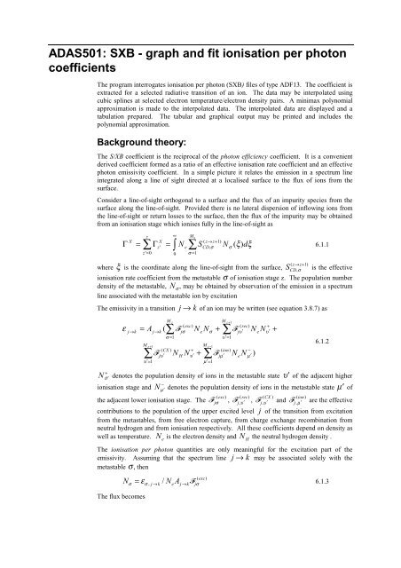
ADAS501: SXB - graph and fit ionisation per photoncoefficientsThe program interrogates ionisation per photon (SXB) files of type ADF13. The coefficient isextracted for a selected radiative transition of an ion. The data may be interpolated usingcubic splines at selected electron temperature/electron density pairs. A minimax polynomialapproximation is made to the interpolated data. The interpolated data are displayed and atabulation prepared. The tabular and graphical output may be printed and includes thepolynomial approximation.Background theory:The S/XB coefficient is the reciprocal of the photon efficiency coefficient. It is a convenientderived coefficient formed as a ratio of an effective ionisation rate coefficient and an effectivephoton emissivity coefficient. In a simple picture it relates the emission in a spectrum lineintegrated along a line of sight directed at a localised surface to the flux of ions from thesurface.Consider a line-of-sight orthogonal to a surface and the flux of an impurity species from thesurface along the line-of-sight. Provided there is no lateral dispersion of inflowing ions fromthe line-of-sight or return losses to the surface, then the flux of the impurity may be obtainedfrom an ionisation stage which ionises fully in the line-of-sight asΓXz∑X= Γ =z'= 0z'∞∫0Mz∑N S N ( ξ)dξ 6.1.1eσ = 1( z→ z+1)CD,σσ( → +1)z zwhere ξ is the coordinate along the line-of-sight from the surface, S CD , σis the effectiveionisation rate coefficient from the metastable σ of ionisation stage z. The population numberdensity of the metastable, N σ, may be obtained by observation of the emission in a spectrumline associated with the metastable ion by excitationThe emissivity in a transition j→ k of an ion may be written (see equation 3.8.7) asεj→k= AM z + 1∑υ′=1j→k)(Mz∑σ = 1( CX )jυ′)N( exc)jσHN+υ′N+eNσM z −1∑µ ′= 1+)M z + 1∑υ′=1( ion)jµ′)N( rec)jυ′eN−µ ′N)eN+υ′+6.1.2+Nϑ ′denotes the population density of ions in the metastable state υ ′ of the adjacent higher−ionisation stage and Nµ ′( rec)( CX ) ( ion)the adjacent lower ionisation stage. The ) , ) , ) and ) are the effectivedenotes the population density of ions in the metastable state µ ′ of(exc)jσcontributions to the population of the upper excited level j of the transition from excitationfrom the metastables, from free electron capture, from charge exchange recombination fromneutral hydrogen and from ionisation respectively. All these coefficients depend on density aswell as temperature. N eis the electron density and N Hthe neutral hydrogen density .The ionisation per photon quantities are only meaningful for the excitation part of theemissivity. Assuming that the spectrum line j→ k may be associated solely with themetastable σ, thenThe flux becomesNσ ε N A )σ , j→k/ej→k( exc)jσj,υ′j,υ ′j , µ′= 6.1.3

ΓX===Mz∑σ = 1Mz∑z∑σ = 1Γ=∞ Mz∫∑0 σ = 1σ , j→k∞∫σ , j→kσ = 1 0M( z)σ6;%6;%[ SIε( z→z + 1)CD,σσ , j→kσ , j→k/ Aj→k( ξ ) dξ)( exc)jσ] εσ , j→k( ξ ) dξ6.1.4whereM z+1( exc)σ j k CDj k j ∑ CDj k)jσυ′=1( z→z + 1)( exc)( z→z + 1)6;%, →S, σ/( A→)σ) = S, σ →υ′ /( A→= 6.1.5and it is assumed that the 6;% coefficient is approximately constant over the region ofemission and may be taken outside the integral. Iσ, j→ kis the line-of-sight integratedemissivity. S CD,σ→υ′is the generalised collisional radiative coefficient from the metastable σof the ion to the metastable υ ′ of the next ionisation stage and S CD,σthe sum over all υ ′.The coefficient is associated therefore with a particular spectrum line and a particularmetastable of the selected ion. It depends on electron density and electron temperature ingeneral.)Resolution levelA specific ion file may be specified at the LS or LSJ resolution levels. That is the populationsof terms or J sub-levels are evaluated with the emissivities being correspondingly of multipletsor multiplet components. Specific ion files in ADAS for low stages of ionisation typical ofinflowing species are usually of LS resolution. Nonetheless, observations at high resolutionmay be of individual components. Consider terms indexed by I and K with their componentlevels indexed by i and k so that i∈Iand k ∈ K. It may be assumed for low stages ofionisation that the level populations of a term are relatively statistically populated. ThenIwAwAI I→Kσ, I→Kσ,i→ki i→kI= 6.1.6where w iis the statistical weight of the level i and w Ithat of term I. Alternatively, if thecomponent observations are complete, I = ∑ I may be obtained fromσ, I→K σ,i→kik ,experiment. The I σ, I→Kare used with term resolved 6;%σ ,I →Kfrom the ADAS database.Non-orthogonal line emissivitiesThe situation of equation 6.1.2 when a spectrum line emission depends on more than onemetastable can occur and the sum over metastables must be retained for the emissivity. Toobtain the fluxes in the separate metastables of the stage z, is is necessary to observe M zlineemissivities which are linearly independent. Generalising the expressionεForm the matrixM z( exc)ρ= Aρ( ∑) jσNeNσ) ρ = 1,.., Mz6.1.7σ = 1( z)σ6;% S CD/ A1=5σ 1−1= and its inverse 5 = 6;% thenρσ , σ ρ)ρσI11+5σ 2I21+ ... +5Γ 6.1.8σM zAll the coefficients of the matrix 6;% are provided in the ADAS database in the metastableresolved case.IM z()

!!S/XB data are extracted from archived files of type ADF13. They are interpolated by cubicsplines in electron temperature and density to provide results at an arbitrary set oftemperature/density pairs. The interpolated data are approximated by a minimax polynomialand a graph produced. A tabulation of the the interpolated spline data and the minimaxapproximation is prepared.Figure 6.1Program steps:These are summarised in figure 6.1.EHJLQ6HOHFW 6;% ILOH!5HDG DQGYHULI\ 6;%ILOH(QWHU ILW FKRLFHV! VHOHFW WUDQVLWLRQDQG RXWSXW WHPS!GHQVLW\ SDLUV&RPSXWH WZR VSOLQH DQGPLQLPD[ ILWVUHSHDWUHSHDW2XWSXW WDEOHVDQG JUDSKVHQG'LVSOD\ 6;%FRHIILFLHQWJUDSKV6HOHFW WDEXODUDQG JUDSKLFDORXWSXW RSWLRQVInteractive parameter comments:Programs of this series (ADAS5) which make use of data from archived ADAS datasetsinitiate an interactive dialogue with the user in three parts, namely, input file selection, entry ofuser data and disposition of output.The file selection window has the appearance shown below1. Data root a) shows the full pathway to the appropriate data subdirectories. Clickthe Central Data button to insert the default central ADAS pathway to the correctdata type. Note that each type of data is stored according to its ADAS data format(adf number). Click the User Data button to insert the pathway to your own data.Note that your data must be held in a similar file structure to central ADAS, butwith your identifier replacing the first adas, to use this facility.2. The Data root can be edited directly. Click the Edit Path Name button first topermit editing.N. B. Under the IDL Graphical User Interface which controls the windowoperations, you must remember to press the return key on the keyboard forany change to be recorded.3. Available sub-directories are shown in the large file display window b). Scrollbars appear if the number of entries exceed the file display window size.4. Click on a name to select it. The selected name appears in the smaller selectionwindow c) above the file display window. Then its sub-directories in turn aredisplayed in the file display window. Ultimately the individual datafiles arepresented for selection. Datafiles all have the termination .dat.5. Once a data file is selected, the set of buttons at the bottom of the main windowbecome active.6. Clicking on the Browse Comments button displays any information stored with theselected datafile. It is important to use this facility to find out what is broadlyavailable in the dataset. The possibility of browsing the comments appears in thesubsequent main window also.

$'$6 ,1387,QSXW 'DWDVHW'DWD URRWSDFNDJHVDGDVDGDVDGI&HQWUDO GDWD 8VHU GDWD (GLW 3DWK 1DPHDV[EEHV[EEHBOOUEHGDWV[EEHBOOUEHGDWV[EEHBOOUEHGDWF'DWD )LOHE%URZVH &RPPHQWV &DQFHO 'RQH7. Clicking the Done button moves you forward to the next window. Clicking theCancel button takes you back to the previous windowThe processing options window has the appearance shown below8. An arbitrary title may be given for the case being processed a). For informationthe full pathway to the dataset being analysed is also shown. The button Browsecomments again allows display of the information field section at the foot of theselected dataset, if it exists.9. The output data extracted from the datafile, in the case of ADAS503, an‘emissivity coefficient’, may be fitted with a polynomial. This is as a function oftemperature. Clicking the Fit polynomial button b) activates this. The accuracyof the fitting required may be specified in the editable box. The value in the boxis editable only if the Fit Polynomial button is active. Remember to press thereturn key on the keyboard to record the value.10. Spectrum lines for which emissivity coefficients are available in the data set aredisplayed in the line list display window. This is a scrollable window using thescroll bar to the right of the window. Click anywhere on the row for a line toselect it. The selected line appears in the selection window c) just above the linelist display window.11. Your settings of electron temperature/electron density pairs (outputs) are shown inthe temperature/density display window d). The temperature and density values atwhich the emissivity coefficients are stored in the datafile (inputs) are also shownfor information. Note that you must give temperature/density pairs, ie. thesame number of each as for a model. The underlying datafile has a twodimensionalstorage as a function of temperature and density.12. The program recovers the output temperature/density pairs you used when lastexecuting the program. Pressing the Default Temperature values button inserts adefault set of temperatures equal to the input temperatures, all at the same density.A choice of density from the input density set is allowed on a ‘pop-up’ window.13. The Temperature & Density Values are editable. Click on the Edit Table button ifyou wish to change the values. A ‘drop-down’ window, the ADAS Table Editor

window, appears as shown below:$'$6 352&(66,1* 237,2167LWOH IRU UXQ'DWD ILOH QDPH GHPRQVWUDWLRQSDFNDJHVDGDVDGDVDGIV[EEHV[EEHBOOUEHGDW%URZVH FRPPHQWVD3RO\QRPLDO )LWWLQJ)LW 3RO\QRPLDO YDOXH E6HOHFW GDWD EORFN,QGH[ :DYHOHQJWK ,RQ 3URFHVVLQJ 0HWDVWDEOH6RXUFH &RGH ,QGH[ $ :-'%( $'$6 F $ :-'%( $'$6 $ :-'%( $'$6 $ :-'%( $'$6 $ :-'%( $'$6 $ :-'%( $'$6 7HPSHUDWXUH'HQVLW\ 9DOXHV7HPSHUDWXUH'HQVLW\,QGH[ 2XWSXW ,QSXW 2XWSXW ,QSXW ( ( ( ( ( ( ( ( ( ( ( ( ( ( ( ( ( ( ( ( ( ( ( ( ( ( ( ( ( ( ( (G7HPSHUDWXUH XQLWV H9 'HQVLW\ XQLWV FP(GLW 7DEOH'HIDXOW 7HPSHUDWXUH YDOXHV&DQFHO'RQHThe output options window appearance is shown below14. As in the previous window, the full pathway to the file being analysed is shownfor information. Also the Browse comments button is available.15. Graphical display is activated by the Graphical Output button a). This will causea graph to be displayed following completion of this window. When graphicaldisplay is active, an arbitrary title may be entered which appears on the top line ofthe displayed graph. By default, graph scaling is adjusted to match the requiredoutputs. Press the Explicit Scaling button b) to allow explicit minima and maximafor the graph axes to be inserted. Activating this button makes the minimum andmaximum boxes editable.

$'$6 287387 237,216'DWD ILOH QDPH SDFNDJHVDGDVDGDVDGIV[EEHV[EEHBOOUEHGDW%URZVH FRPPHQWV*UDSKLFDO 2XWSXW'HIDXOW 'HYLFHD*UDSK 7LWOHGHPRQVWUDWLRQ+3*/([SOLFLW 6FDOLQJ;PLQ

Figure 6.1aTable 6.1aADAS RELEASE: ADAS93 V1.7 PROGRAM: ADAS501 V1.7 DATE: 31/07/96 TIME: 21:12*** TABULAR OUTPUT FROM IONIZATIONS PER PHOTON INTERROGATION PROGRAM: ADAS501 - DATE: 31/07/96 ***------------------- -------------------IONIZATIONS PER PHOTON AS A FUNCTION OF ELECTRON TEMPERATURE AND DENSITY-------------------------------------------------------------------------DATA GENERATED USING PROGRAM: ADAS501-------------------------------------FILE :/packages/adas/adas/adf13/sxb93#be/sxb93#be_llr#be0.dat - DATA-BLOCK: 3EMITTING ION INFORMATION:-------------------------ELEMENT NAME= BERYLLIUMELEMENT SYMBOL= BENUCLEAR CHARGE (Z0) = 4CHARGE STATE (Z) = 0WAVELENGTH (angstroms) = 3326.1 ASPECIFIC ION FILE SOURCE = WJD91#BEPROCESSING CODE= ADAS208METASTABLE INDEX = 1--- ELECTRON TEMPERATURE --- ELECTRON DENSITY IONIZATIONSkelvin eV cm-3 PER PHOTON1.161D+04 1.000D+00 1.000D+12 3.730D-022.321D+04 2.000D+00 1.000D+12 4.040D-015.803D+04 5.000D+00 1.000D+12 3.280D+00. . .7.544D+05 6.500D+01 1.000D+12 1.300D+029.284D+05 8.000D+01 1.000D+12 1.910D+02-------------------------------------------------------------------------------NOTE: * => IONIZATIONS PER PHOTON EXTRAPOLATED FOR TEMPERATURE/DENSITY VALUE-------------------------------------------------------------------------------MINIMAX POLYNOMIAL FIT TO ELECTRON TEMPERATURES - TAYLOR COEFFICIENTS:-------------------------------------------------------------------------------- LOG10(IONIZATIONS PER PHOTON) versus LOG10(ELECTRON TEMPERATURE) --------------------------------------------------------------------------------A( 1) = -1.410628476D+00 A( 2) = 3.767911738D+00A( 3) = -1.524257187D+00 A( 4) = 8.502256577D-02A( 5) = 1.096116453D-01LOGFIT - DEGREE= 4 ACCURACY= 4.15% END GRADIENT: LOWER= 3.77 UPPER= 1.91-------------------------------------------------------------------------------Notes: