NUMERICAL METHODS FOR THE TRIDIAGONAL HYPERBOLIC ...

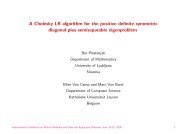
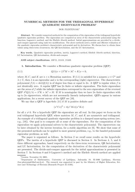
NUMERICAL METHODS FOR THE TRIDIAGONAL HYPERBOLICQUADRATIC EIGENVALUE PROBLEM ∗BOR PLESTENJAK †Abstract. We consider numerical methods for the computation of the eigenvalues of the tridiagonal hyperbolicquadratic eigenvalue problem. The eigenvalues are computed as zeros of the characteristic polynomial using thebisection, Laguerre’s method, and the Ehrlich–Aberth method. Initial approximations are provided by a divideand-conquerapproach using rank two modifications. The above methods need a stable and efficient evaluation ofthe quadratic eigenvalue problem’s characteristic polynomial and its derivatives. We discuss how to obtain thesevalues using three-term recurrences, the QR factorization, and the LU factorization.Key words. Quadratic eigenvalue problem, inertia, Laguerre’s method, Ehrlich–Aberth method, bisection,LU factorization, QR factorization, divide-and-conquerAMS subject classifications. 65F15, 15A18, 15A69.1. Introduction. We consider a Hermitian quadratic eigenvalue problem (QEP)(1.1)Q(λ)x = (λ 2 M + λC + K)x = 0,where M,C, and K are n × n Hermitian matrices. If (1.1) is satisfied for a nonzero x ∈ C n andλ ∈ C, then λ is an eigenvalue and x is the corresponding (right) eigenvector. The characteristicpolynomial f(λ) = det(Q(λ)) is of degree less than or equal to 2n. A QEP is regular when f isnot identically zero. A regular QEP has 2n finite or infinite eigenvalues. The finite eigenvaluesare the zeros of f while the infinite eigenvalues correspond to the zero eigenvalues of the reversedQEP λ 2 Q(1/λ) = λ 2 K + λC + M. If M is nonsingular then we have 2n finite eigenvalues withup to 2n eigenvectors, which are not necessarily linearly independent. QEPs appear in variousapplications, for a recent survey of the QEP see [19].We say that a QEP is hyperbolic [11] if M is positive definite and(x ∗ Cx) 2 > 4(x ∗ Mx)(x ∗ Kx)for all x ≠ 0. For a hyperbolic QEP the eigenvalues are all real. In this paper we focus on thereal tridiagonal hyperbolic QEP, where matrices M, C, and K are symmetric and tridiagonal.An example of a tridiagonal quadratic eigenvalue problem is a damped mass-spring system (see,e.g., [19]). Our goal is to compute all or some of the eigenvalues. For the computation of theeigenvalues we apply polynomial solvers to the characteristic polynomial. The eigenvectors canbe later obtained by the inverse iteration, for a stable algorithm see [6]. We show that some ofthe presented methods can be applied to more general problems, e.g., to the banded polynomialeigenvalue problems, as well.The paper is organized as follows. In Section 2 we recall some results on the hyperbolicQEPs. The inertia of a hyperbolic QEP is discussed in Section 3. In Sections 4, 5, and 6three different approaches, based respectively on the three-term recurrences, QR factorization,and LU factorization, for the computation of the derivatives of the characteristic polynomialare presented. The divide-and-conquer approach for the initial approximations is presented inSection 7. In Sections 8 and 9 Laguerre’s method and the Ehrlich–Aberth method are applied∗ Version: November 19, 2005.† Department of Mathematics, University of Ljubljana, Jadranska 19, SI-1000 Ljubljana, Slovenia(bor.plestenjak@fmf.uni-lj.si). The research was supported in part by the Ministry of Higher Education, Scienceand Technology of Slovenia (Research Project Z1-3136).1

2 B. PLESTENJAKto the computation of the zeros of the characteristic polynomial, respectively. Some numericalexamples are given in Section 10, followed by conclusions.2. Auxiliary results. The following properties of the hyperbolic QEPs are gathered from[7, 11, 16]. A hyperbolic QEP has 2n real eigenvalues and eigenvectors. All eigenvalues aresemisimple and there is a gap between the largest n (primary) and the smallest n (secondary)eigenvalues. There are n linearly independent eigenvectors associated with the primary and thesecondary eigenvalues, respectively.For each x ≠ 0 the equationµ 2 x T Mx + µx T Cx + x T Kx = 0has two distinct real solutions µ 1 (x) < µ 2 (x). If x is an eigenvector, then at least one of µ 1 (x)and µ 2 (x) is the corresponding eigenvalue. Values µ 1 (x) and µ 2 (x) are generalizations of theRayleigh quotient and similar to the symmetric matrices there exists minimax theorem for thehyperbolic QEP as well.Theorem 2.1 (Duffin [7]). If λ 2n ≤ · · · ≤ λ 1 are the eigenvalues of a hyperbolic QEP thenλ n+i = maxS⊂R ndim(S)=imin µ 1(x) and λ i = max0̸=x∈S S⊂R ndim(S)=imin µ 2(x)0̸=x∈Sfor i = 1,... ,n.Theorem 2.2 (Markus [16]). A Hermitian QEP where M is positive definite is hyperbolicif and only if there exists γ ∈ R such that the matrix Q(γ) is negative definite.Remark 2.3. The scalar γ in Theorem 2.2, such that Q(γ) is negative definite, lies in thegap between the primary and the secondary eigenvalues, i.e., λ n+1 < γ < λ n .3. Inertia of a hyperbolic QEP. The inertia of a symmetric matrix A is a triplet ofnonnegative integers (ν,ζ,π), where ν,ζ, and π are respectively the number of negative, zeroand positive eigenvalues of A. The following theorem shows that the inertia of a symmetricmatrix Q(σ) is related to the number of eigenvalues of the QEP Q that are larger or smallerthan σ, respectively.Theorem 3.1. Let M,C, and K be symmetric n × n matrices such that Q(λ) = λ 2 M +λC + K is a hyperbolic QEP and let λ 2n ≤ · · · ≤ λ n+1 < λ n ≤ · · · ≤ λ 1 be the eigenvalues of theQEP Q. If (ν,ζ,π) is the inertia of the matrix Q(σ) then ζ is the algebraic multiplicity of σ asan eigenvalue of the QEP Q anda) if σ > λ n then ν is the number of eigenvalues of Q larger than σ and π+n is the numberof eigenvalues of Q smaller than σ,b) if σ < λ n+1 then ν is the number of eigenvalues of Q smaller than σ and π + n is thenumber of eigenvalues of Q larger than σ.Proof. For each λ ∈ R, Q(λ) is a symmetric n × n matrix with n real ordered eigenvalues(3.1)µ n (λ) ≤ · · · ≤ µ 1 (λ),where µ 1 ,... ,µ n are continuous functions of λ. It is easy to see that σ is an eigenvalue of theQEP Q of algebraic multiplicity k exactly when there exists 1 ≤ i ≤ n such thatµ i (σ) = µ i+1 (σ) = · · · = µ i+k−1 (σ) = 0.Since M is a symmetric positive definite matrix,limλ→±∞ µ i(λ) = ∞

NUMERICAL METHODS FOR THE HYPERBOLIC QEP 3for all i. By Theorem 2.2 there exists σ 0 ∈ R such that µ i (σ 0 ) < 0 for all i. Because each µ i isa continuous function it has at least two zeros, one on the right and one on the left side of σ 0 .As each zero of µ i is also an eigenvalue of the QEP Q which has 2n eigenvalues, it follows thateach µ i has exactly two zeros.As µ 1 ,... ,µ n are continuous and ordered as in (3.1), it is not hard to deduce that if σ > σ 0and σ is not an eigenvalue of Q then the number of negative eigenvalues of Q(σ) equals thenumber of eigenvalues of Q that are larger than σ. This proves a) and similarly we can proveb).Remark 3.2. Theorem 3.1 is a generalization of a similar theorem in [18], where M is apositive definite matrix and K is a negative definite matrix. In this case Q(0) is negative definiteand a proof similar to the above can be done without applying Theorem 2.2.Based on the inertia we could apply the bisection to obtain the kth eigenvalue. The algorithmis similar to the algorithm for the symmetric eigenvalue problem. To derive more efficientmethods, we use some faster methods that were successfully applied to tridiagonal eigenvalueproblems: Laguerre’s method [14, 15] and the Ehrlich–Aberth method [4].The above methods need stable and efficient computation of ν(Q(λ)), f(λ), f ′ (λ)/f(λ) andf ′′ (λ)/f(λ), where f(λ) = det(Q(λ)). We discuss how to obtain these values using the three-termrecurrences, the QR factorization, and the LU factorization in the next three sections.4. Three-term recurrences. Let Q(λ) = (λ 2 M +λC +K), where M,C, and K are n ×ntridiagonal matrices. We can write⎡a 1 (λ) b 1 (λ) 0⎤b 1 (λ) a 2 (λ) b 2 (λ)Q(λ) =.⎢ .. . .. . ..⎥⎣b n−2 (λ) a n−1 (λ) b n−1 (λ)⎦ ,0 b n−1 (λ) a n (λ)where a i (λ) = λ 2 M ii + λC ii + K ii and b i (λ) = λ 2 M i+1,i + λC i+1,i + K i+1,i are quadratic polynomials.The determinant of a tridiagonal matrix can be computed using a three-term recurrence,see, e.g., [9]. If f k (λ) = det(Q k (λ)), where Q k (λ) is the leading k × k submatrix of Q(λ), thenandf r+1 = a r+1 f r − b 2 rf r−1 ,f 0 = 1, f 1 = a 1 ,f 0 ′ = 0, f 1 ′ = a ′ 1 ,f 0 ′′ = 0, f 1 ′′ = a ′′1 ,f ′ r+1 = a ′ r+1f r + a r+1 f ′ r − 2b r b ′ rf r−1 − b 2 rf ′ r−1,f ′′r+1 = a ′′r+1f r + 2a ′ r+1f ′ r + a r+1 f ′′r − 2b ′2r f r−1 − 2b r b ′′rf r−1 − 4b r b ′ rf ′ r−1 − b 2 rf ′′r−1for r = 1,... ,n − 1. For the sake of brevity the argument λ is omitted in the above equations.As the above recurrences may suffer from overflow and underflow problems [13], we defined i = f if i−1,g i = f i′ , h i = f i′′.f i f i

4 B. PLESTENJAKThen f n = d 1 · · · d n ,andd r+1 = a r+1 − b2 rd r,d 1 = a 1 ,g 0 = 0, g 1 = a′ 1a 1,h 0 = 0, h 1 = a′′ 1a 1,g r+1 = 1d r+1(a ′ r+1 + a r+1 g r − 1 d r(2b r b ′ r + b 2 rg r−1 )h r+1 = 1d r+1(a ′′r+1 + 2a′ r+1 g r + a r+1 h r − 1 d r(2b ′2r + 2b rb ′′r + 4b rb ′ r g r−1 + b 2 r h r−1)for r = 1,... ,n − 1.Remark 4.1. One can see that d 1 ,...,d n are the diagonal elements from the LDL T factorizationof the matrix Q(λ).Remark 4.2. The algorithm may break down if d r = 0 for some r = 1,... ,n − 1. In suchcase we introduce small perturbations and setd r =),εd r−1(|λ| 2 |M r−1,r−1 | + |λ||C r−1,r−1 | + |K r−1,r−1 | + ε ) ,where ε is the machine precision. This corresponds to a small relative perturbation of the matricesM, C, and K. A similar approach is used in [14].5. A QR factorization approach. If f(λ) ≠ 0 then it follows from Jacobi’s formula forthe derivative of the determinant that)(5.1)f ′ (λ)/f(λ) = tr(Q(λ) −1 Q ′ (λ)).If we denote A = Q(λ) and B = Q ′ (λ), then we need to compute tr(A −1 B), where in our caseA and B are tridiagonal matrices. In [4] one can find a stable O(n) computation of tr(A −1 ) viaQR factorization. In this section we generalize this algorithm to compute tr(A −1 B). We startwith a sketch of the algorithm for tr(A −1 ), for details and the theory, see [4].Let A be a tridiagonal matrix and let A = UR, where⎡⎤r 1 s 1 t 1. .. . .. . ..R =⎢ r n−2 s n−2 t n−2 ⎥⎣r n−1 s⎦n−1r nis an upper triangular tridiagonal matrix and U is the product of n − 1 Givens rotations,U ∗ = G n−1 · · · G 2 G 1 , where[ ]ψi θG i ([i,i + 1],[i,i + 1]) = iand |ψ−θ i ψ i | 2 + |θ i | 2 = 1.i

NUMERICAL METHODS FOR THE HYPERBOLIC QEP 5Thenwhere⎡⎤v 1 u 1 ψ 1 0v 2 u 1 v 2 u 2 ψ 2U ∗ .=. . .. . ..,⎢⎥⎣ . v n−1 u n−1 ψ n−1⎦v n u 1 v n u 2 · · · v n u n−1 v n u nIf we solve Rw = v, then(5.2)D = diag(1, −ψ 1 ,ψ 1 ψ 2 ,...,(−1) n−1 ψ 1 ψ 2 · · · ψ n−1 ),u = D −1 [1,θ 1 , · · · ,θ n−1 ] T ,v = D[θ 1 , · · · ,θ n−1 ,1] T .tr(A −1 ) =n∑u i w i .Kressner [10] generalized the above approach into an O(n) algorithm for the computation oftr(A −1 B), where both matrices A and B are tridiagonal. Suppose that⎡⎤x 1 z 1 0y 1 x 2 z 2B =. .. . .. . ..⎢⎥⎣y n−2 x n−1 z⎦ .n−10 y n−1 x nTo compute tr(A −1 B) we need the diagonal elements of A −1 B. Fromandit follows that(5.3)tr(A −1 B) =(A −1 B) ii = e T i R−1 U ∗ Be i= z i−1 e T i R−1 U ∗ e i−1 + x i e T i R−1 U ∗ e i + y i e T i R−1 U ∗ e i+1 ,i=1e T i R −1 U ∗ e i−1 = u i−1 w i ,e T i R −1 U ∗ e i = u i w i ,e T i R−1 U ∗ e i+1 = u i+1 w i + 1 r i(ψ i − v i u i+1 )n∑z i−1 u i−1 w i +i=2n∑i=1n−1∑x i u i w i + y i(u i+1 w i + 1 )(ψ i − v i u i+1 ) .r iAs reported in [4], formula (5.2) is not stable. To make it stable, we have to avoid the explicitmultiplication by the matrix D or D −1 . If we define ˆR = D −1 RD, ˆv = D −1 v, û = Du, andsolve ˆRŵ = ˆv for ŵ, then(5.4)tr(A −1 ) =i=1n∑û i ŵ i .i=1

NUMERICAL METHODS FOR THE HYPERBOLIC QEP 7Algorithm 6.1 (Bohte [5]). The algorithm solves the equation B = MU + LV for M andV , where L is a lower triangular matrix with ones on the main diagonal, U is a nonsingularupper triangular matrix, B is a square n × n matrix, M is a lower triangular matrix with zeroson the main diagonal, and V is an upper triangular matrix.for r = 1 to nfor k = r to nv rk = b rk − ∑ r−1j=1 (m rju jk + l rj v jk )for i = r + 1 to(nm ir = 1u rrb ir − ∑ )r−1j=1 (m iju jr + l ij v jr ) − l ir v rrFor the second derivative we have(6.2)PQ ′′ = L ′′ U + 2L ′ U ′ + LU ′′ = NU + 2MV + LW,where N = L ′′ is a lower triangular matrix with zeros on the diagonal and W = U ′′ is an uppertriangular matrix. It follows thatf ′′ (λ)f(λ) = n∑i=1( n∑w ii+u iii=1v iiu ii) 2−n∑v 2 iiu 2 i=1 iiFrom the relation (6.2) we get PQ ′′ − 2MV = NU + LW, which means that we can applyAlgorithm 6.1 for the computation of N and W as well.An implementation of Algorithm 6.1 for banded matrices computes f ′ /f and f ′′ /f in alinear time. The algorithm is more expensive than the three-term recurrences in Section 4, butits advantage is that it can be applied to non-tridiagonal matrices as well. Let us also mentionthat in [5] one can find a slightly modified algorithm that is able to compute f ′ (λ) even iff(λ) = 0.7. Divide-and-conquer. We choose m ≈ n/2 and writeQ(λ) = Q 0 (λ) + b m (λ)(e m−1 e T m+1 + e m+1e T m−1 ),.whereQ 0 (λ) =[ ]Q1 (λ) 0.0 Q 2 (λ)Q 0 (λ) is a rank two modification of Q(λ). If we apply Theorem 2.2 then it is not hard to seethat Q 1 and Q 2 are hyperbolic QEPs. The eigenvalues ˜λ 2n ≤ · · · ≤ ˜λ 1 of Q 0 , a union of theeigenvalues of Q 1 and Q 2 , are approximations to the eigenvalues λ 2n ≤ · · · ≤ λ 1 of Q.We can show that the eigenvalues of Q 0 and Q interlace. To show this useful property weintroduce a convex combination of Q 0 and Q. Let Q t be a QEP defined byQ t (λ) = (1 − t)Q 0 (λ) + tQ(λ).Lemma 7.1. The QEP Q t is hyperbolic for t ∈ [0,1].Proof. From Theorem 2.2 it follows that there exists γ such that Q(γ) is negative definite.Being principal submatrices of Q(γ), matrices Q 1 (γ) and Q 2 (γ) are negative definite as well.Since it is a block diagonal matrix with negative definite blocks Q 1 (γ) and Q 2 (γ), matrix Q 0 (γ)

NUMERICAL METHODS FOR THE HYPERBOLIC QEP 9Point b) follows from Lemma 7.2. We know that λ i and ˜λ i are connected by a monotoneeigencurve λ i (t), which is bounded below and above by ˜λ i+1 and ˜λ i−1 , respectively.Remark 7.4. Unlike the divide-and-conquer method for the symmetric tridiagonal matrices,here ˜λ i = ˜λ i+1 does not imply that one of the eigenvalues of Q is ˜λ i . Only if ˜λ i−1 = ˜λ i = ˜λ i+1then one can deduce that ˜λ i is an eigenvalue of Q.In the conquer phase we use a numerical method that computes the eigenvalues λ 1 ,...,λ 2nof the QEP Q from the initial approximations ˜λ 1 ,... , ˜λ 2n . Two numerical methods that maybe applied for this task are presented in the next two sections. We are not claiming that theseare the optimal methods. Other polynomial solvers applied to the classical or to the generalizedeigenvalue problem with tridiagonal matrices (see, e.g., [12, 17]) could be applied to the QEPas well.8. Laguerre’s method. To the characteristic polynomial f(λ) = det(Q(λ)) we can applyLaguerre’s method, a well-known globally convergent method for finding polynomial zeros. Onestep of Laguerre’s iteration is(8.1)L ± (x) = x + ⎛2n√ √√√(2n (⎝ −f ′ (x)f(x) ± − 1) (2n − 1)( −f ′ (x)f(x)) ) ⎞ 2− 2n f ′′ (x)⎠.f(x)For more details on the method and its properties see, e.g., [14, 20].For a polynomial having all real roots the method is globally convergent with a cubic convergencein a neighborhood of a simple eigenvalue. If we add λ 2n+1 = −∞ and λ 0 = ∞ then forx ∈ (λ i+1 ,λ i ) we haveλ i+1 < L − (x) < x < L + (x) < λ i .In the divide-and-conquer algorithm we use Laguerre’s method to compute the eigenvaluesλ 2n ≤ · · · ≤ λ 1 of Q from the initial approximations ˜λ 2n ≤ · · · ≤ ˜λ 1 that are the eigenvaluesof Q 0 . We know from Theorem 7.3 that ˜λ i+1 ≤ λ i ≤ ˜λ i−1 and that we can use ˜λ i as an initialapproximation for λ i . From ν(Q(˜λ i )) we see if λ i > ˜λ i or ˜λ i < λ i and then use the appropriateL + or L − sequence. The global convergence of Laguerre’s method guarantees that we get allthe eigenvalues by computing them independently one by one.Although the convergence close to a simple eigenvalue should be cubic, we can expect veryslow convergence at the beginning if ˜λ i is closer to λ i−1 or λ i+1 than to λ i (see Figure 8.1).λ i+2 λ i+1 λ i λ i-1~λ i+1~λ i~λ i-1Fig. 8.1. Slow convergence can occur when ˜λ i is much closer to λ i−1 or λ i+1 than to λ i. The cubic convergenceregion around a simple eigenvalue λ i.

NUMERICAL METHODS FOR THE HYPERBOLIC QEP 11The main stopping criteria is the relative size of a correction. We take ε = 10 −15 and stopthe iteration for λ j when|λ (k+1)j− λ (k)j| ≤ |λ (k+1) |ε.Another stopping criteria for Laguerre’s method are different inertias of Q(λ (k+1)j) and Q(λ (k)j).In the Ehrlich-Aberth method we use a heuristic that stops the iteration once the large majorityof the eigenvalues has converged and the corrections for the remaining eigenvalues stop becomingsmaller.In both methods one step (an iteration for one eigenvalue approximation) has linear timecomplexity. If we compare the number of operations needed for the equations (8.1) and (9.1),and for the three-term recurrences in Section 4, then we can observe that one step of Laguerre’smethod is more expensive and is roughly equivalent to 1.8 Ehrlich–Aberth steps.Example 10.1. In the first numerical example we use random tridiagonal matrices, wherethe elements are uniformly distributed in such intervals that the obtained QEP is hyperbolic.For the matrices M and K, the diagonal and codiagonal elements are uniformly distributedin [0.5,1] and [0,0.1], respectively. The diagonal and codiagonal elements of the matrix C areuniformly distributed in [4,5] and [0,0.5], respectively.n Ehrlich-Aberth R Ehrlich-Abert C Laguerre-bisection ZGGEVaverage number of iterations in the last D&C100 1.88 1.89 1.86200 1.76 1.76 2.09400 1.57 1.58 1.20800 1.55 1.54 1.26time in seconds100 0.02 0.03 0.02 0.60200 0.05 0.13 0.06 5.02400 0.13 0.39 0.23 52.95800 0.48 1.48 0.83 684.63maximum relative error100 5e-15 4e-16 5e-15 5e-14200 5e-15 4e-16 5e-15 9e-14400 5e-15 4e-16 5e-15 1e-13800 5e-15 4e-16 5e-15 1e-13Table 10.1The average number of iterations in the last divide-and-conquer step, the computational time, and the maximumrelative error of the computed eigenvalues in Example 10.1.jThe numerical results are presented in Table 10.1. In the first two columns are the resultsfor the Ehrlich–Aberth method; in the first column we use real arithmetic while in the secondcolumn we use complex perturbations and complex arithmetic. Complex perturbations increasethe computational time for one iteration but in some cases (see, e.g., Example 10.2), where wehave multiple or close eigenvalues, we might have faster convergence. In the third column arethe results for Laguerre’s method and in the last column are the results for the Lapack routineZGGEV applied to the linearized generalized eigenvalue problem (10.1) of size 2n. The costof ZGGEV, which is not optimized for block tridiagonal matrices, is O(n 3 ) compared to O(n 2 )for the methods presented in this paper. Because of that ZGGEV is slower from the presentedmethods even for a moderate size of matrices.We tested the methods on matrix dimensions from 100 to 800. The results in Table 10.1 areorganized in three parts. In the upper part is the average number of iterations in the last divideand-conquerstep. For Laguerre’s method we count bisection steps as well. As the dimension

12 B. PLESTENJAKof the matrices increases, better the eigenvalues of Q 0 (λ) approximate the eigenvalues of Q(λ)and fewer iterations are needed in the final phase. The middle part in Table 10.1 contains thecomputational times in seconds. One can see that although Laguerre’s method needs feweriterations, it runs slower than the Ehrlich–Aberth method which does not compute the secondderivatives. In the lower part of the table are the maximum relative errors of the computedeigenvalues. In this example all methods perform well and give small relative errors. Themaximum condition number of the eigenvalues (for the definition, see, e.g., [19]) in Example10.1 is of order 10 3 .Example 10.2. In this example we use matrices with constant diagonals and codiagonals,such that the QEP is hyperbolic. We take M = tridiag(0.1,1,0.1), C = tridiag(0.5,5,0.5), andK = tridiag(0.2,1,0.2). For such problem the eigenvalues can be computed analytically. Alleigenvalues are simple, but we can expect problems in the divide-and-conquer approach becausethe eigenvalues of Q 0 appear in pairs. The eigenvalues are not very sensitive, the maximumcondition number for the eigenvalues in this example is of order 10 2 .Numerical results, organized in the same way as in Example 10.1, are presented in Table 10.2.We can see that the number of iterations is larger than in Example 10.1. The Ehrlich–Aberthmethod has problems with close initial approximations. In this case Laguerre’s method givesthe best performance.n Ehrlich-Aberth R Ehrlich-Abert C Laguerre-bisection ZZGEVaverage number of iterations in the last D&C100 19.93 18.49 5.75200 19.57 17.55 5.70400 18.98 17.05 5.67800 18.46 16.50 5.64time in seconds100 0.08 0.22 0.03 0.64200 0.33 0.92 0.13 5.33400 1.30 3.70 0.53 58.42800 5.17 14.59 2.09 865.13maximum relative error100 3e-15 5e-16 3e-15 6e-15200 3e-15 5e-16 3e-15 5e-15400 3e-15 6e-16 3e-15 2e-14800 3e-15 6e-16 3e-15 3e-15Table 10.2The average number of iterations in the last divide-and-conquer step, the computational time, and the maximumrelative error of the computed eigenvalues in Example 10.2.Example 10.3. The Ehrlich–Aberth method in complex arithmetic can also be applied tothe QEPs that are not hyperbolic and where the eigenvalues might be complex. The interlacingproperty of the eigenvalues of Q 0 and Q is no longer true, but we can still expect that theeigenvalues of Q 0 are good initial approximations to the eigenvalues of Q. When the solutionsare complex, Laguerre’s method is not globally convergent anymore and without the inertia andthe interlacing property we have no guarantee that the method returns all the eigenvalues.For the first nonhyperbolic QEP we use random symmetric tridiagonal matrices. The diagonalelements of matrices M, C and K are uniformly distributed in [0,1]. The codiagonalelements of matrices M, C, and K are uniformly distributed in [0,0.1], [0,0.5], and [0,0.2],respectively. The maximum condition number of the eigenvalues is of order 10 9 and this reflectsin larger errors than in the other examples.For the second nonhyperbolic QEP we use an example from [19], where M = tridiag(0.1,1,0.1),

NUMERICAL METHODS FOR THE HYPERBOLIC QEP 13C = tridiag(−3,9, −3), and K = tridiag(−5,15, −5). All eigenvalues are simple, but the eigenvaluesof Q 0 are double. The maximum condition number of the eigenvalues is of order 10 3 .Numerical results in Table 10.3 show that the Ehrlich–Aberth can be applied to such QEPs.QEP 1 QEP 2ZZGEV Ehrlich–Aberth C ZZGEV Ehrlich–Aberth Cn time error time avg. iter error time error time avg. iter error100 0.75 4e-13 0.03 1.94 1e-13 0.59 7e-15 0.23 20.10 2e-15200 6.16 3e-12 0.11 1.72 9e-15 5.23 4e-14 1.02 19.52 2e-15400 67.09 4e-12 0.39 1.56 4e-14 46.64 6e-14 4.09 18.88 4e-15Table 10.3The average number of iterations in the last divide-and-conquer step, the computational time, and the maximumrelative error of the computed eigenvalues in Example 10.3.Example 10.4. We consider the second-order model of vibration of a rotating axel in apower plant from [2]. We have a second-order differential equationM ¨z + Cż + Kz = Du,where M, C, and K are tridiagonal symmetric matrices of dimension n = 211. The norms ofthe matrices are ‖M‖ = 1.7 · 10 3 , ‖C‖ = 2 · 10 2 , and ‖K‖ = 1.5 · 10 12 . One eigenvalue of thecorresponding QEP is 0, which makes the resulting system neither observable nor detectable.The largest real part of the remaining nonzero eigenvalues is ρ = −0.01626718.If we apply the Ehrlich–Aberth method, then the relative error of the computed ρ is of order10 −14 . The average number of iterations in the last divide-and-conquer step is 6.8. If we use thelinearization (10.1) and ZGGEV then the relative error of the computed ρ is of order 10 −6 . Ifwe reduce the linearized 422 ×422 problem into a 421 ×421 problem for the nonzero eigenvaluesas in [2] then the relative error of the computed ρ rises to 10 −9 . This example shows that wecan get more accurate results without a linearization. The eigenvalues in this example havecondition numbers of orders from 10 4 up to 10 10 .Example 10.5. The above ideas can be extended to QEPs with banded matrices as well. Wecan apply the Ehrlich-Aberth method as long as we have an efficient method for the computationof the characteristic polynomial and its derivative. For banded matrices these values can becomputed in a linear time using the algorithm based on the LU factorization from section 6.As in the previous examples, the initial approximations are obtained by the divide-andconquerscheme. The matrices M, C, and K are represented as 2 × 2 block matrices and thenthe approximations are obtained by a recursive application of the method to the diagonal blocksubproblems.p n = 50 n = 100 n = 2001 3.91 2.85 2.322 5.78 4.18 3.313 6.23 5.31 4.444 6.42 5.91 5.335 9.27 6.44 6.37Table 10.4The average number of iterations in the last divide-and-conquer step for the banded quadratic eigenvalueproblem with matrices of dimension n and bandwidth p from Example 10.5.The following example was done in Matlab 7.0. We take three matrices of dimension n withnormally distributed elements: M=randn(n), C=randn(n), and K=randn(n), set m ij = c ij =

14 B. PLESTENJAKk ij = 0 for |i − j| > p, where p is the bandwidth, and apply the Matlab implementation of theEhrlich-Aberth method.As expected, the results in Table 10.5 show that the average number of iterations in the lastdivide-and-conquer step does increase with the bandwidth. However, for a small bandwidth,one step is performed in linear time and the results in Table 10.5 show that the Ehrlich-Aberthmethod can be considered as an alternative for the banded quadratic eigenvalue problems. Forall combinations of p and n in Table 10.5 the maximum relative error of the computed eigenvaluesis below 10 −14 and smaller from the error obtained by the Matlab function polyeig that appliesQZ to the linearized problem.11. Conclusions. We have presented two numerical methods for the tridiagonal hyperbolicQEP that use the divide-and-conquer approach. Both methods can be easily parallelized. Laguerre’smethod and bisection require hyperbolicity, while the Ehrlich–Aberth method might beapplied to more general problems, for instance, nonsymmetric tridiagonal quadratic eigenvalueproblems, tridiagonal polynomial eigenvalue problems, banded polynomial eigenvalue problems,and others. In these applications, the algorithm based on the LU factorization might be usedfor an efficient computation of the derivative of the determinant.Let us mention that at the moment there are no methods for transforming a general QEPto a tridiagonal form. In future, this might change with structure preserving transformations(SPT) [8].Acknowledgements. The author would like to thank Daniel Kressner for providing thegeneralization of the QR factorization approach in Section 5. The author would also like tothank Dario Bini and Françoise Tisseur for useful suggestions and comments. The author is alsograteful to the referees for careful reading of the paper and several helpful comments.REFERENCES[1] E. Anderson et al., LAPACK user’s guide. Third edition, SIAM, Philadelphia, 1999.[2] J. Abels and P. Benner, DAREX - a collection of benchmark examples for discrete-time algebraic Riccatiequations (version 2.0), SLICOT Working Note 1999-16, 1999.[3] D. A. Bini, Numerical computation of polynomial zeros by means of Aberth’s method, Numerical algorithms13, (1996), pp. 179–200.[4] D. A. Bini, L. Gemignani, and F. Tisseur, The Ehrlich–Aberth method for the nonsymmetric tridiagonaleigenvalue problem, SIAM J. Matrix Anal. Appl., 27 (2005), pp. 153–175.[5] Z. Bohte, Calculation of the derivative of the determinant, Obzornik mat. fiz. 28, (1981), pp. 33–50.[6] I. R. Dhillon, Reliable computation of the condition number of a tridiagonal matrix in O(n) time, SIAMJ. Matrix Anal., 19 (1998), pp. 776–796.[7] R. J. Duffin, A minimax theory for overdamped networks, J. Rational Mech. Anal., 4 (1955), pp. 221–233.[8] S. D. Garvey, Structure preserving transformations for linear dynamic systems, available athttp://www.nottingham.ac.uk/~eazsg/SPT/index.htm.[9] G. H. Golub, C. F. van Loan, Matrix computations, 3rd ed., Johns Hopkins University Press, Baltimore,1996.[10] D. Kressner, personal communication (2003).[11] P. Lancaster, Quadratic eigenvalue problems, Linear Algebra Appl., 150 (1991), pp. 499–506.[12] K. Li, Durand–Kerner root-finding method for the generalized tridiagonal eigenproblem, Missouri J. Math.Soc., (1999), pp. 33–43.[13] K. Li and T. Y. Li, An algorithm for symmetric tridiagonal eigenproblems: Divide and conquer withhomotopy continuation, SIAM J. Sci. Comput., 14 (1993), pp. 735–751.[14] T. Y. Li and Z. Zeng, Laguerre’s iteration in solving the symmetric tridiagonal eigenproblem - revisited,SIAM J. Sci. Comput., 15 (1994), pp. 1145–1173.[15] K. Li, T. Y. Li, and Z. Zeng, An algorithm for generalized symmetric tridiagonal eigenvalue problems,Numerical Algorithms, 8 (1994), pp. 269–291.

NUMERICAL METHODS FOR THE HYPERBOLIC QEP 15[16] A. S. Markus, Introduction to the spectral theory of polynomial operator pencils, Amer. Math. Soc.,Providence, 1988.[17] V. Pereyra and G. Scherer, Eigenvalues of symmetric tridiagonal matrices: a fast, accurate and reliablealgorithm, J. Inst. Math. Applics., 12 (1973), pp. 209–222.[18] D. Sapagovene, The Sturm sequence for a nonlinear algebraic eigenvalue problem, Upravlenija I sekcijaVYP, 16 (1976), pp. 87–95.[19] F. Tisseur and K. Meerbergen, The quadratic eigenvalue problem, SIAM Review, 43 (2001), pp. 235–286.[20] J. Wilkinson, Algebraic eigenvalue problem, Oxford University Press, Oxford, 1965.