Leiby - NESUG

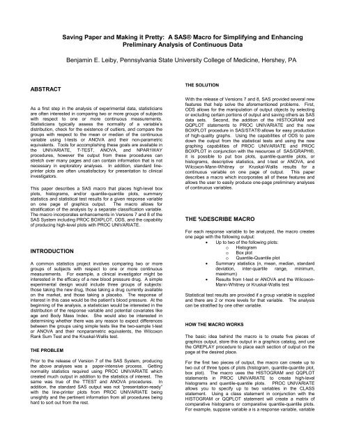
Saving Paper and Making it Pretty: A SAS® Macro for Simplifying and EnhancingPreliminary Analysis of Continuous DataBenjamin E. Leiby, Pennsylvania State University College of Medicine, Hershey, PAABSTRACTAs a first step in the analysis of experimental data, statisticiansare often interested in comparing two or more groups of subjectswith respect to one or more continuous measurements.Statisticians typically assess the normality of a variable’sdistribution, check for the existence of outliers, and compare thegroups with respect to the mean or median of the continuousvariable using t-tests or ANOVA and their non-parametricequivalents. Tools for accomplishing these goals are available inthe UNIVARIATE, T-TEST, ANOVA, and NPAR1WAYprocedures, however the output from these procedures canstretch over many pages and can contain information that is notnecessary in exploratory analyses. In addition, standard lineprinterplots are often unsatisfactory for presentation to clinicalinvestigators.This paper describes a SAS macro that places high-level boxplots, histograms, and/or quantile-quantile plots, summarystatistics and statistical test results for a given response variableon one page of graphics output. The macro allows forstratification of the analysis by a separate classification variable.The macro incorporates enhancements in Versions 7 and 8 of theSAS System including PROC BOXPLOT, ODS, and the capabilityof producing high-level plots with PROC UNIVARIATE.INTRODUCTIONA common statistics project involves comparing two or moregroups of subjects with respect to one or more continuousmeasurements. For example, a clinical investigator might beinterested in the efficacy of a new blood pressure drug. A simpleexperimental design would include three groups of subjects:those taking the new drug, those taking a drug currently availableon the market, and those taking a placebo. The response ofinterest in this case would be the patient’s blood pressure. At thebeginning of the analysis, a statistician would be interested in thedistribution of the response variable and potential covariates likeage and Body Mass Index. She would also be interested indetermining whether there was any reason to expect differencesbetween the groups using simple tests like the two-sample t-testor ANOVA and their nonparametric equivalents, the WilcoxonRank Sum Test and the Kruskal-Wallis test.THE PROBLEMPrior to the release of Version 7 of the SAS System, producingthe above analyses was a paper-intensive process. Gettingnormality statistics required using PROC UNIVARIATE whichcreated much output in addition to the statistics of interest. Thesame was true of the TTEST and ANOVA procedures. Inaddition, the standard SAS output was not “presentation-ready”with the line-printer plots from PROC UNIVARIATE beingunsightly and the pertinent information from all procedures beinghard to sort out from the rest.THE SOLUTIONWith the release of Versions 7 and 8, SAS provided several newfeatures that help solve the aforementioned problems. First,ODS allows for the manipulation of output objects by selectingor excluding certain portions of output and saving others as SASdata sets. Second, the addition of the HISTOGRAM andQQPLOT statements to PROC UNIVARIATE and the newBOXPLOT procedure in SAS/STAT® allows for easy productionof high-quality graphs. Using the capabilities of ODS to paredown the output from the statistical tests and using the newgraphing capabilities of PROC UNIVARIATE and PROCBOXPLOT in conjunction with the resources of SAS/GRAPH®,it is possible to put box plots, quantile-quantile plots, orhistograms, descriptive statistics, and t-test or ANOVA, andWilcoxon-Mann-Whitney or Kruskal-Wallis results for acontinuous variable on one page of output. This paperdescribes a macro which incorporates all of these features andallows the user to easily produce one-page preliminary analysesof continuous variables.THE %DESCRIBE MACROFor each response variable to be analyzed, the macro createsone page with the following output:•= Up to two of the following plots:o Histogramo Box ploto Quantile-Quantile plot•= Summary statistics (n, mean, median, standarddeviation, inter-quartile range, minimum,maximum)•= Results from t-test or ANOVA and the Wilcoxon-Mann-Whitney or Kruskal-Wallis testStatistical test results are provided if a group variable is suppliedand there are 2 or more levels for that variable. The analysiscan be stratified by one other variable.HOW THE MACRO WORKSThe basic idea behind the macro is to create five pieces ofgraphics output, store this output in a graphics catalog, and usethe GREPLAY procedure to place each section of output on thepage at the desired place.For the first two pieces of output, the macro can create up totwo out of three types of plots (histogram, quantile-quantile plot,box plot). The macro uses the HISTOGRAM and QQPLOTstatements in PROC UNIVARIATE to create high-levelhistograms and quantile-quantile plots. PROC UNIVARIATEallows you to specify up to two variables in the CLASSstatement. Using a class statement in conjunction with theHISTOGRAM or QQPLOT statement will create a matrix ofcomparative histograms or comparative quantile-quantile plots.For example, suppose variable a is a response variable, variable

•=•=•=•=VAR = A list of the continuous variables to be analyzedGROUP = The variable that identifies the group to which anobservation belongs. This is the class variable for the t-testor ANOVA. Only one variable can be specified.BY = The variable used to stratify the analysis. Only one byvariable can be specified. For readability of the output, a byvariable should have no more than four levels.GRAPHS = HISTOGRAM | BOXPLOT | QQPLOT | NONEThe macro allows the user to choose which plots will appearin the output. The user may choose up to 2 of the three plottypes. If more than two are specified, only the first two willbe used. Specify NONE to exclude the graphical output. Bydefault, the macro produces histograms and box plots.•= VARPAGE = 1 | 2This is the number of variables to put on a page of output. IfVARPAGE=1, one variable's output is placed on an entirepage. If VARPAGE=2, each variable's output is placed onhalf of the page. By default, the macro puts output for onevariable on each page.•=MAXDEC = The maximum number of decimal places for thedescriptive statistics. The default value is 3.(Washington County, Maryland; Forsyth County, North Carolina;and selected suburbs of Minneapolis, Minnesota). The fourthpart of the cohort was sampled from black residents of Jackson,Mississippi. Demographic information including race, age, sex,alcohol use, smoking status, and education level was collected.Subjects underwent a medical examination at the beginning ofthe study and one every three years thereafter to determine thepresence of cardiopulmonary diseases including coronary heartdisease and to record relevant health information including bodymass index (BMI), blood pressure and presence ofhypertension, diabetes, and cholesterol level.ANALYSISAs a first step, we might want to check our randomization andsee if the distribution of age is similar across the fourcommunities. To use the macro, we would choose age as ourresponse variable and center as our group variable. Thefollowing macro call asks for an analysis of age by center.%describe(data=chd,var=age, group=center,graphs=boxplot qqplot, varpage=1, maxdec=1,device=pdf, gfile=example1.pdf,rotate=portrait);The output can be seen in Figure 5.•=•=•=•=•=DEVICE = The graphics device used to produce the finaloutput. By default, the current graphics device (as specifiedwith a GOPTIONS statement) is used. If no graphics devicehas been specified, the macro will use the device PS1200 (apostscript driver).GFILE = The graphics file where the output will be stored.By default, the current graphics output file (specified with theGSFNAME option in the GOPTIONS statement) is used.DENSITY= KERNEL | NORMAL | BOTH | NONESpecify which density estimate curves to plot on thehistograms. By default, the macro will produce both kerneldensity estimates and a normal density curve. The kerneldensity estimate is based on the normal distribution.REPLACE= REPLACE | APPENDSpecifies whether to replace the specified graphics file withthe pages produced by the current macro call or to appendthose pages to the graphics file. This is especially usefulwhen calling the macro more than once in a program. Bydefault, the macro will replace the specified graphics file.ROTATE= PORTRAIT | LANDSCAPESpecifies the orientation of the final plot. By default, themacro uses portrait orientation.Another concern might be possible differences between thosewith coronary heart disease and those without disease withrespect to the continuous risk factors, controlling for center. Themacro call would be:%describe(data=chd, var=age bmi cholesterolglucose dbp sbp, group=chd, by=center,graphs=histogram boxplot, varpage=1, maxdec=3,device=pdf, gfile=example2.pdf,rotate=landscape);This macro call will generate six pages of output, one for eachvariable specified in the var= parameter. Pages 2 and 4 of theoutput are found in Figures 6 and 7. Notice the difference inoutput layout with the landscape orientation.ADDITIONAL INFORMATION:In order to accommodate PROC GPRINT, the macro writes thestatistical output to two text files. This macro was written for useon a Unix platform and includes commands to delete the filesafter they are used. If used on a different platform, these linesshould be commented out:x rm –f tests.txt;x rm –f stats.txt;EXAMPLEDATA DESCRIPTIONThe data set used in these examples is a random sample fromthe Atherosclerosis Risk in Communities (ARIC) study cohort.The ARIC study, sponsored by the National Heart, Lung, andBlood Institute, is a community-based, longitudinal study ofcardiovascular and pulmonary diseases. The ARIC cohort wasselected as a probability sample of 15,792 men and womenbetween the ages of 45-64 year at four study centers in theUnited States, three of which enumerated and enrolled all ageeligibleresidents sampled from geographically defined areasWhile the macro will work for most types of graphics devicedrivers, it was designed with postscript and PDF drivers in mind.When using a Windows-related driver like CGM, only oneanalysis variable should be specified in the VAR= option. Usingweb-related drivers will often produce undesirable results,especially when using group and by variables with more than 3levels. The size of the print becomes too small to be seen withthe coarser resolutions of most web-related drivers.The macro calls two graphics macros (%SIZEIT and%TMPLTMAC to replay the box plots. These macros areaccessed using the SASAUTOS and MAUTOSOURCE options.The SASAUTOS option needs to be changed depending on thelocation of the macros and the platform on which the program isrun.

CONCLUSIONACKNOWLEDGMENTSWith the new tools provided in Versions 7 and 8 of the SASSystem, it is possible to produce a one-page summary ofpreliminary statistical analyses of continuous variables. This caninclude high-quality statistical plots, descriptive statistics, andresults from statistical tests. The %DESCRIBE macro can dothese things easily, allowing the user to analyze numerouscontinuous variables grouped by one variable and stratified byanother with one macro call. The output can be presentedwithout embarrassment and with little confusion to nonstatisticianinvestigators.Many thanks to Dr. David Mauger, Assistant Professor ofBiostatistics in the Department of Health Evaluation Sciences,for providing the idea for this macro and to Linda Engle and AmyMatthews, Statistical Analysts in the Department of HealthEvaluation Sciences, for assisting in macro testing. Specialthanks to Dr. Duanping Liao, Assistant Professor ofEpidemiology, for providing the data and data description for theexamples.CONTACT INFORMATIONREFERENCESARIC investigators. “The atherosclerosis risk in the communities(ARIC) study: Design and objectives.” American Journal ofEpidemiology, 1989; 129:687-702Curtis, Nathan A. “Are Histograms Giving You Fits? New SASSoftware for Analyzing Distributions.”www.sas.com/rnd/app/papers/distributionanalysis.pdfWatts, Perry. “Managing SAS/GRAPH Displays with theGREPLAY Procedure.” Proceedings of the NorthEast SAS UsersGroup, Inc. 11 th Annual Conference, 439-445.Your comments and questions are valued and encouraged.Send feedback and requests for the macro code to:Benjamin E. LeibyThe Pennsylvania State UniversityCollege of MedicineDepartment of Health Evaluation Sciences, A210P.O. Box 855Hershey, PA 17033-0855Work Phone: 717.531.7178Fax: 717.531.5779Email: bleiby@hes.hmc.psu.eduSAS, SAS/STAT, and SAS/GRAPH are registered trademarksof SAS Institute, Inc. in the USA and in other countries. ®indicates USA registration.

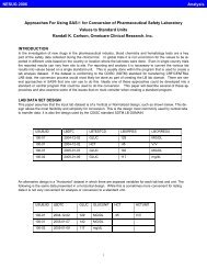
Figure 5. Analysis of Age grouped by Study Center

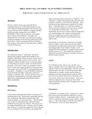
Figure 6. Analysis of BMI grouped by Disease Status and stratified by Study Center

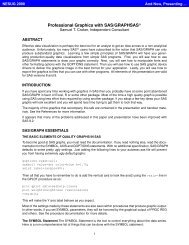
Figure 7. Analyzing Fasting Glucose grouped by Disease Status and stratified by Study Center