Dummy Variables and the Relationship of Deaf and ... - NESUG

NESUG 2008Statistics & AnalysisDummy Variables and the Relationship of Deaf and Hearing Growth Using SAS/GRAPH®Rich Dirmyer, Scannell & Kurz, Inc, Rochester, NYSara Schley, RIT/NTID Office of the Vice President & Dean, Rochester, NYAbstractHistorically, deaf education in the United States has achieved poor results. An oft-quoted statistic is that on average, deafstudents graduating from high school (at age 18-21) perform at the level of hearing 8-10 year olds in terms of reading andwriting skills (Allen, 1994; Traxler, 2000). In this research, deaf children and their hearing siblings from a longitudinaldatabase are tracked during their elementary and secondary school years. This presentation will focus on graphic displays ofthe longitudinal data, focusing on presenting individual data points and sub-group regression lines on a single graph (here,one regression line for the deaf sample, and one for the hearing siblings), tracking their school progress from K-12. Thesedisplays inform statistical data analysis. Detailed examples of code will be shared, as well as insights into the value ofcombining graphic displays with data analysis.IntroductionThis paper includes an intermediate presentation of statistical analysis, using regression methods. Individuals who have beenexposed to predictive modeling in the mathematical or statistical sense should feel comfortable attending this session. TheGLM, GPLOT, and GREPLAY Procedures in Base SAS® and SAS/GRAPH® were used in this paper.The StudyIn order to determine statistically significant differences in educational development between hearing and deaf children, fourassessments where used. These scores measure basic math, verbal, and reading abilities from adolescence to early adulthood.The following four Peabody assessments were used:The Peabody Individual Achievement Test for Math measures basic mathematical ability. It is one of the more widely usedassessments of individual academic achievement.The Peabody Individual Achievement Test in Reading Comprehension measures a child’s ability to derive the meaning ofpassages read silently.The Peabody Individual Achievement Test in Reading Recognition measures a child’s word recognition and pronunciationabilities. Children were asked to read a word silently, and then say it aloud for an administrator.The Peabody Picture Vocabulary Test is an assessment given to children that measures their hearing vocabulary for Englishwords and provides an estimate of their verbal ability based on it.The data supplied included scores for hearing children, as well as their deaf/hard of hearing siblings. Using sibling’s dataremoves the potential unwanted variation from family to family. It is worth noting that the sample size changes fromvariable to variable due to missing data points. However sample sizes from n=221 to n=341 were maintained.To determine differences between hearing and deaf children, linear models will be constructed in which age is the predictor,and the scores in question are the response. As of now, if age was regressed onto scores, the linear model would be achieved,but wouldn’t be comparable to anything. Therefore, dummy variables will be implemented to separate the overall regressionline into two unique regression lines, one for the deaf sample, and one for the hearing sample.1

NESUG 2008Statistics & AnalysisMethod of AnalysisSometimes in statistics, variables have two or more distinct levels, such as machines or operators. Often times thesevariables are referred to as categorical variables. In order to properly analyze the data using these types of variables, onemust take into account the fact that variables with multiple levels may have separate deterministic effects on the responsevariable. In situations like this, the implementation of dummy variables is highly useful.There are many ways to set up dummy variables so long as they are linearly independent of other variables in the model. Theparticular set up used in this research codes deaf = 1 and hearing = 0. It should be said that a variable with a levels willemploy the use of a-1 dummy variables. Since the study only concerns deaf and hearing siblings, only one dummy variableis necessary.As stated before, only one dummy variable was needed. The general model that will be constructed takes on the form:Y (o 1 0 1X= β + β X ) + Z ( α + α ) + εIn the model Z represents the dummy variable, and it can be seen that if Z=0 the hearing model becomes:and when Z=1 the deaf model becomes:Y = β + X 10βY = β + α ) + ( β + )X(0 0 1α1Now with two regression models, differences between the deaf and hearing samples can be tested. It is easy enough to showthe two samples are in fact different yet something else may be shown. A difference only concludes that there are tworegression lines present, but does not show how the lines differ from one another. Four situations arise:Situation 1: Two distinct regression models with different slopes, and different intercepts (4 parameters).Situation 2: Two distinct regression models with equal slopes, and different intercepts (3 parameters).Situation 3: Two distinct regression models with different slopes, and equal intercepts (3 parameters).Situation 4: One distinct regression line with equal slopes and equal intercepts (2 parameters).Identifying one of these situations gives even more information than a simple difference between the two samples. Thesesituations tell us whether or not deaf and hearing siblings begin at the same levels, or different levels, and whether or not theyprogress at the same, or a different rate. As an aid to the analysis performed on the data, scatter plots have been provided.AnalysisIn order to test each situation, the appropriate F-tests must be constructed using extra sums of squares (ESS). The ESS aresimply calculated as:ESSTest Parameter= SSRe gression− SSParametersnot testedThat is, the extra sums of squares that are produced by the addition of the respective test parameters. Once the ESS areobtained, the formal F-test may be performed as in any ANOVA or regression analysis.Fortunately, SAS produces tests based on these ESS, which it calls Type III Sums of Squares. The trick in obtaining theType III SS for a regression model involves using The GLM Procedure. The following code was used to obtain the necessarytests for deciding which situation is present:2

NESUG 2008Statistics & AnalysisData RichD.Dualsample;input age deaf_flag ;interaction = age*deaf_hear;Run;Proc Glm Data=RichD.Dualsample;model = age deaf_flag interaction / SS3;Run;The lack of the CLASS statement in PROC GLM treats each independent variable in the model as one degree of freedom,essentially fitting a regression model rather than an additive model. The SS3 option in the model statement suppresses theType I Sums of Squares and produces the ESS needed to draw conclusions. Example output resulting from the code lookslike:Sum ofSource DF Squares Mean Square F Value Pr > FModel 3 42005.30802 14001.76934 88.55 Fage 1 25495.25056 25495.25056 161.23

NESUG 2008Statistics & AnalysisGoptions Reset=All Device=GIF;Symbol1 Color=Blue Interpol=None Value=Circle Height=1 Width=1;Symbol2 Color=Red Interpol=None Value=Square Height=1 Width=1;Axis1 Order=(0 to 20 by 1)Label=(Color=black Height=2 'Age')Major=(Height=1) Minor=NoneWidth=2;Axis2 Order=(0 to n by i)Label=(Color=black Angle=90 Height=2 'Name of Test')Major=(Height=1) Minor=NoneWidth=2;Legend1 Label=(Color=Black Height=2 'Population')Value=(Color=Blue Height=2 'Deaf' 'Hearing')Across=1 Down=2Position=(Top Left Inside)Mode=Share;Since the graphs produced were treated as static graphs, they were stored as GIF files using the DEVICE= option whichprovide no opportunity for interactivity, and take up minimal space. Two SYMBOL statements were used in order todistinguish between the deaf and hearing sample. Colors, as well as shapes were used using the COLOR= and VALUE=options respectively to represent each sample as first a visual pleaser, and then in the event of the document printed in blackand white, visual separation.Axes were then set using appropriate scales. The only assessment which does not follow the same scaling in scores is thePeabody Picture Vocabulary Test, so the only modification necessary in the above code is the ORDER= option of the y-axis.Also, in the AXES2 statement, the label was rotated 90 degrees using the ANGLE= option in order to keep the graphs cleanlooking and compact.Lastly, a legend was created which was given the dimension 2 x 1 using the ACROSS= and DOWN= options, and positionedin the upper left corner of the graph, with MODE=share specified. This last option ensures that the legend does not cover anydata points which may impede the space where the legend was positioned.Now, with the appropriate options specified, The GPLOT procedure was run.Proc GPlot Data=RichD.DualPlot;Plot *deaf_age *hearing_age /Overlay Legend=Legend1NoFrameHaxis=axis1Vaxis=axis2;Quit;In order to visually detect which situation is present, both populations were plotted on the same graphing window using theoverlay option. Lastly, The GREPLAY procedure was used to condense the four graphs into one window.Proc GReplay igout=work.gseg tc=sashelp.templt template=L2R2 nofs;Treplay 1:gplot 2:gplot1 3:gplot2 4:gplot3;Quit;4

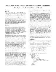
NESUG 2008Statistics & AnalysisAs each graph is created in PROC GPLOT, it is stored in the work.gseg directory, with naming conventions related to thecreation order of each graph. PROC GREPLAY allows users to augment graphs into matrix plots if desirable, giving usersnumerous templates to choose from, which are located in the sashelp.templt directory. The template chosen for this paper isthe L2R2 template, which intuitively creates a square 2 x 2 matrix plot. Using the TREPLAY statement determines theplacement of the specified graphs, and as a result, the following matrix plot is obtained.Popul at i onDeafHeari ngPopul at i onDeafHeari ngAgeAgePopul at i onDeafHeari ngPopul at i onDeafHeari ngAgeAgeAs a recap, the graph displaying the PIAT Math scores shows that there are in fact two distinct regression models, withdifferent slopes and same intercepts. Therefore, among deaf and hearing siblings, both start off at the same level regardingmathematical ability, however hearing siblings develop their math skills at a quicker rate than their deaf siblings. Regarding,the Peabody Picture Vocabulary Test, there are two distinct regression models, and the deaf and hearing siblings progress atthe same rate, yet begin at different levels. As for the PIAT in Reading Recognition, there are two distinct regression modelswith different slopes and different intercepts. Graphically, it appears that the hearing sample starts off at a higher level, andprogresses at a quicker rate. Lastly, the PIAT in Reading Comprehension shows the same situation as the recognition testing,however in this case, the deaf sample begins at a higher level than the hearing sample.ConclusionThis study revealed interesting points about the relationship between deaf and hearing development. The use of the SASsystem’s graphing and regression capabilities gives users a new approach to classic regression problems. The GPLOTprocedure allows users to interpret the statistical conclusions in a concise manner with supporting visuals. While the datadoes not indicate that high school deaf children perform at a level of 8-10 year olds, the deaf sample scores did increase at aslower rate than the hearing sample in each of the four assessments.5

NESUG 2008Statistics & AnalysisReferencesTraxler, Carol Bloomquist. 2000 Fall. “The Stanford Achievement Test, 9 th Edition: National Norming and PerformanceStandards for Deaf and Hard-of-Hearing Students”. Journal of Deaf Studies and Deaf Education. 5(4): 337-348.Bureau of Labor Statistics. “National Longitudinal Surveys”. http://www.bls.gov/nlsSAS® and all other SAS Institute Inc. product or service names are registered trademarks or trademarks of SAS Institute Inc,in the USA and other countries. ® indicates USA registration.AcknowledgementsSAS and all other SAS Institute Inc. product or service names are registered trademarks of SAS Institute Inc, in the USA andother countries. ® indicates USA registration.The research outlined in this document was supported by NSF Career Award #REC0346951 – “Deaf Children and YoungAdults: Predicting School, College and Labor Success.”Special thanks to:The individuals of Scannell & Kurz, Inc. and their endless support of their employees.My beautiful wife Roselle Dirmyer, and her endless support of my research and career objectives.Contact InformationRich DirmyerScannell & Kurz, Inc.71-B Monroe AvenuePittsford, NY 14534Work Phone: 585-381-1120E-mail: dirmyer@scannellkurz.comSara SchleyRIT/NTID Office of the Vice President & Dean52 Lomb Memorial DriveRochester, NY 14623Work Phone: 585-475-7981E-mail: sara.schley@rit.edu6