Drill Down Till You Drop: OLAP Without Windows - NESUG

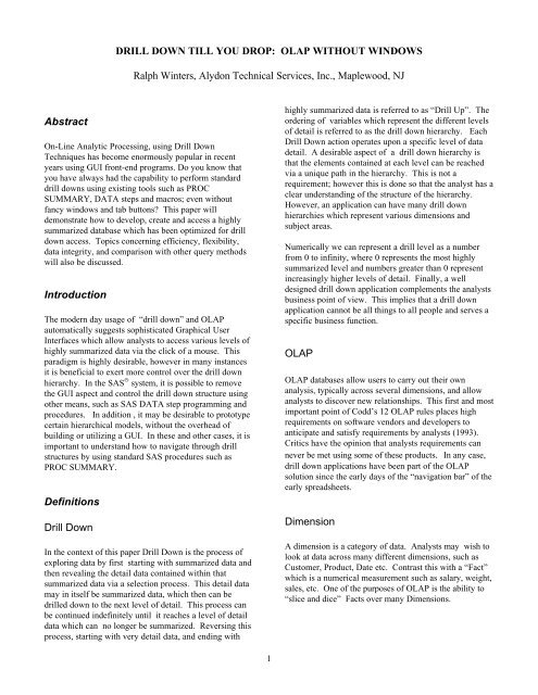
Sample DataA sample demonstration database is used in the exampleswhich consists of 35,000 observations measuring salesfigures collected from various cities in the USA andCANADA. Each observation contains an individual salesamount generated by a specific SALESPERSON for aparticular DATE, COUNTRY, REGION,STATE/PROVINCE, and CITY.Review of PROC SUMMARYPROC SUMMARY is a SAS procedure which canproduce various summary statistics for all numericvariables in a data set. This procedure is well suited toOLAP and drill down applications since it can produceoutput which leads to many different kinds of analyses,both within the same dimension or across differentdimensions. In PROC SUMMARY terminology thevariables listed on the CLASS statement take on attributesof Dimensions, and variables on the VAR statement aretreated as Facts. Data statistics pertaining to Facts canthen be pre-summarized, and then be available foranalysis with minimum impact upon computation time.PROC SUMMARY produces separate summary statisticsfor various subgroups of variables on the CLASSstatement. A subgroup is defined for each individualCLASS variable, as well as for each combination ofCLASS variables. Thus, 3 variables which are listed onthe CLASS statement will generate 8 separate summarysubgroups.The output from PROC SUMMARY is a special data setcontaining summary statistics which have been calculatedfor each variable listed on the VAR statement. Importantpoints regarding this output data set are:• Each observation contains a special _TYPE_ variablewhich identifies the subgroup to which the summarystatistics apply. By examining the _TYPE_ variableas a bitmap variable you can “decode” a specificsubgroup and determine which variables on theCLASS statement define that subgroup.• Each observation contains a _FREQ_ variablerepresenting the number of observations for thatcurrent subgroup.• The observations also contains the CLASS variableswhich represents the subgroup. If a CLASS variabledoes not contribute to the subgroup it is representedas missing.Let’s use the Sample Data Set as an example and set up aPROC SUMMARY with the following code:2PROC SUMMARY data=drill noprint;CLASS city state region;VAR sales;output out=temp sum=;The output dataset “temp” contains 8 observations whichrepresent sales summaries for all the observations in“drill” broken down by every combination of CITY,STATE, and REGION (Table 1). To see how the_TYPE_ variable works, we will look at the _TYPE_variable as a bit string with each bit representing avariable in the CLASS statement. If that bit is “on”, thevariable it represents is included in the subgroup. Therightmost CLASS variable is represented by therightmost bit, the next adjacent CLASS variable to the leftis represented by the next bit to the left, etc. To arrive at ainteger value for _TYPE_ , you multiple the value of eachbit by 2 raised to the K power, where K represents the bitposition, with 0 being the rightmost position andincreasing by 1 for each bit to the left. Sum all of theresults for every CLASS variable as computed above toarrive at a final value for the _TYPE_ variable.The 8 different _TYPE_ variables corresponding to thefollowing subgroups are defined below:Table 1_TYPE_SUBGROUPBITSTRING OFCITY STATE REGION1 REGION 0 0 12 State 0 1 03 Region by State 0 1 14 City 1 0 05 Region by City 1 0 16 State by City 1 1 07 Region by State by City 1 1 10 TOTAL 0 0 0Example:Using Table 1 Above: The Subgroup “Region” iscomputed as:1*2 0 + 0*2 1 + 0*2 2 = 1while Subgroup “State by City” is computed as:0*2 0 + 1*2 1 + 1*2 2 = 6A _TYPE_ variable equal to 0 always represents statisticsrepresenting the total for the entire dataset. For eachdistinct _TYPE_ there will be as many elements in asubgroup as there are levels or combinations of levels forthe contributing CLASS variables. For example, If oursample data set contained only two states: NJ, and MD,

and contained only three cities, Baltimore, Newark, andAnnapolis, there would be two observations correspondingto _TYPE_=2, three observations corresponding to_TYPE_=4, and three observations corresponding to_TYPE=6.Selection of the Dimensions and DrillHierarchySelection of the proper dimensions for the drill downinvolves careful study of analysts needs and anunderstanding of the relationship among the entitieswhich the data represents. In many cases, the drillhierarchy may follow an organizations standard way ofdoing business, but in other cases, the data can be minedfirst using techniques such as CHAID and CART in orderto find significant dimensions for analysis. The entireprocess of determining the needs of the analyst can not beoveremphasized, since the drill down model shouldprovide a meaningful application for the analyst. If not,the model can end up being too simplistic, complex, orsimply wrong from a business point of view.Our sample data will use a Time/Geography Drillhierarchy. Examining the relationship among the levelsthere is a natural relationship as follows:drill downDATE→ COUNTRY→ REGION→STATE/PROVINCE→ CITYdrill upCITY→ STATE/PROVINCE→ REGION→ COUNTRY→ DATEIn other more complex cases there may not be a naturalorder, or the relationship may be a one-to-manyrelationship. In this case more analysis would be needed.Specification of the PROC SUMMARYNext, we will set up a PROC SUMMARY specifying thehierarchy we have established. However, we must takecare when setting up the CLASS statement, since theorder in which the variables appear is important. In orderto take advantage of numerical properties of the _TYPE_variable, we will specify the drill down order in theCLASS statement from right to left. Therefore thestatement for this example becomes:PROC SUMMARY data=drill noprint;CLASS city state region country date ;VAR sales;output out=temp sum=;Note that we also need to select an analysis variable aswell as a summary statistic. Since drill down applicationsneed to access summary statistics at each level of the drillhierarchy, we need to specify SUM= on the outputstatement. We will also specify SALES as the variablewhich is to be summed.Creating the Optimized Drill DownDatasetAs mentioned earlier, the output of PROC SUMMARYwill generated observations for each combination ofCLASS variables listed on the CLASS statement. Eventhough PROC SUMMARY drastically reduces the numberof observations in the output dataset, as compared to theoriginal dataset, in a drill down hierarchy we are onlyinterested in a subset of all possible subgroups. We willexamine the output dataset “temp” to see whichobservations correspond to the drill hierarchy at eachlevel. Those observations will be kept, while others willbe discarded.• We need the summary for DATE by itself(_TYPE_=1) since this is the starting level for ourdrill down.• The next level of drill down is to the COUNTRYlevel. In this case, the required summary would bethe one corresponding to _TYPE_=3 (DATE byCOUNTRY). We will include DATE as part of thissubgroup since we will already have drilled downfrom the starting DATE level, and need the DATEvariable as a way to provide a link to the previouslevel. If we examine all of the other subgroups whichcontain COUNTRY we will find a summary forCOUNTRY by itself, as well as subgroups containingcombinations of variables such as COUNTRY byCITY, COUNTRY by STATE by CITY, etc. Some ofthese summaries will be discarded, since we are onlyinterested in that summary relevant to positionswithin the drill down hierarchy.• If we continue to work through the drill hierarchy tothe next level, we see that the REGION level requires_TYPE_=7 (DATE by COUNTRY by REGION),since by drilling down to the REGION level, we willhave already drilled down on DATE and thenCOUNTRY. By the same rational given for theprevious level, we can discard the other _TYPE_variables containing REGION not relevant to our drilldown. (For example: REGION by CITY will be3

discarded since REGION is never selected by drillingdown on CITY).• If we continue this process to the last variable, CITY,we see that the only _TYPE_ values needed are 1, 3,7, 15 and 31. At each of these levels, the subgroupincludes the CLASS variables corresponding to thevariable at that level, plus all variables which havealready been “drilled down on” in the hierarchy.If we only include these types, how much will that reducethe size of the output dataset? That will depend upon thenumber of distinct levels for each _TYPE_. Referring toTable 2, we can see that we are now left with a datasetcontaining only 68 observations, drastically reducing thenumber of observations in the output summary data set,relative to both the original “drill” dataset, and the output“temp” dataset.Table 2_TYPE_ SUBGROUP OBS1 Date 53 Country by Date 107 Region by Country by Date 1515 State by Region by Country by 34Date31 City by State by Region byCountry by Date34We can generalize the above example by stating that in adrill down hierarchy, where we have N CLASS variableswhich have been arranged in drill down order from rightto left, in order to perform a drill down as describedabove, we only require the output observations which have_TYPE_ values in:{ 2 0 ,2 0 + 2 1 ,2 0 + 2 1 + 2 2 ,2 0 + 2 1 + 2 2 + 2 3 ……….. ,2 0 + 2 1 + 2 2 + 2 3 + 2 N-1 }with 0 being the most rightmost position, and increasingby 1 for each variable to the left. (1.1)Using the output data temp as generated above we createthe optimized drill down dataset by subsetting:data temp;set temp;4where _TYPE_ in (1, 3, 7, 15, 31);A special form of the above formula exists when the drillhierarchy starts from the rightmost variable in the CLASSstatement. In this case the first _TYPE_ value is always1, and the next drill down value is generated bymultiplying the last variable by 2 and adding 1. (1.2)In a “drill-up” situation, this would be equivalent tosubtracting 1 from the current level and then dividing by2.If we still are left with a large output data set, afterreducing the size in this manner, we may choose to placean index on the _TYPE_ variable if it will providesignificantly quicker access to the data.PROC SQL;create index _TYPE_ on temp (_TYPE_);Reordering the Drill HierarchyIt is usually best to set up the order of the drill variablesfrom right to left, as we just did in the preceding example,however it is not essential to do so.Let’s say we were interested in reordering the drillhierarchy starting with COUNTRY, and then drillingdown on DATE, REGION, all the way down to CITY.Our drill hierarchy now becomes:COUNTRY→ DATE→ REGION → STATE→ CITYSince we have already created the optimized database,how does that affect the reordering of the variables ? Wecould always reorder the positions of the drill variablesfrom right to left, and rerun the original PROCSUMMARY etc., but there is another way:If we express our modified drill hierarchy with respect topowers of 2 we have:2 1 → 2 0 → 2 2 → 2 3 → 2 4If we examine the exponent of 2 in each case, we see thatit represents the position, starting with 0, of the level inthe CLASS statement.Since COUNTRY is now the 2nd variable from the righton the CLASS statement, it has a _TYPE_ value of 2 1 , or2. This becomes the first _TYPE_ value. The nextvariable in the hierarchy is DATE, which has a _TYPE_value of 1, so we add these two values together to get thenext _TYPE_ value which is 3. The next level isREGION, so we add the _TYPE_ value of 4 to get the

esult 7. Since the remainder of the hierarchy remains thesame, the set of new _TYPE_ values generated withrespect to the Drill hierarchy now becomes:{2, 3, 7, 15, 31 }Note that now we are applying an additive rule whichadds the value of the next _TYPE_ value to thesummation of the previously accumulated _TYPE_values. (1.3)If we look at the set of {2, 3, 7, 15, 31 }, it does breakour prior rules for generating the _TYPE_ values {1.1,1.2}. That is because the drill hierarchy is not beinginterpreted strictly from right to left.If we had expressed our original example in the format:2 0 → 2 1 → 2 2 → 2 3 → 2 4we could have also used this additive rule to arrive at theidentical series {1 , 3, 7, 15, 31}.Analysis of the optimized data setNow that an optimized drill data set has been created, wecan demonstrate its usage by using simple PROC PRINTstatements with WHERE clauses. Of course, this can beextended to other SAS procedures as well. In order tocontrast this method with the standard GUI interpretationof Drill down, we will contrast each step of the processwith the equivalent GUI application step. For thisexample we will use the sample data set described above.Drilling Down - The Traditional GUI Way1. We open up an GUI application which contains salesdata for the sample data set described.2. A list box which contains months and associatedsales data for that month is displayed (Table 3).3. Select May 97 from the list of available months anddrill down to the next level which displays a list boxcontaining sales data for the USA and CANADA(Table 4).4. Select USA from the list of countries to drill down tothe next level displaying the sales data for the 2regions NE, SE (Table 5).5. Select NE from the list of regions to display the salesdata for the 3 states in the Northeast CT, NJ, and NY(Table 6).6. Select NJ to display the sales figures for Trenton, theonly city in the territory with sales data for May 97(Table 7).7. We realize that we neglected to note the sales totalsfor the states in the Northeast, so we click the“BACK” button to get to the previous screen, andnote the totals for the states (Table 6).Table 3 Table 4Jan 97 33,000,000 CAN 8,000,000Feb 97 36,000,000 USA 24,300,000Mar 97 36,000,000Apr 97 34,000,000May 97 32,300,000Table 5NE 12,000,000SE 12,300,000Table 6 Table 7CT 6,000,000 Trenton 1,000NJ 1,000,000NY 5,000,000Drilling Down - The Windowless Way1. There is no front end application to open up. Weopen up an interactive SAS session, and assign thecorrect LIBNAMES for the datasets.2. To obtain a list of sales months and sales generated,corresponding to step 2 above, we first need todetermine which level we will start at. In this case itis the DATE level, and we already have establishedthat this corresponds to _TYPE_=1:Proc print data=temp;var date sales;where _TYPE_=1;Switching to the output window reveals all of the monthsand sales figures which correspond to the resultsillustrated in Table 3 above. Although the displaymethods are completely different in both cases, theinformation is identical.3. In the previous illustration we selected 01MAY97from the list of available with a mouse. Let’ssimulate the selection of a month in our “windowless”environment.Proc print data=temp;var country sales;where month=’01MAY97’D and _TYPE_=3;5

• The month which is being selected issupplied via the WHERE statement.• The next drill down level is also supplied inthe WHERE statement via the _TYPE_variable. But in order to determine the valueof that _TYPE_ variable, we first need tocompute the value of the next drill downlevel. From our earlier algorithm (1.2), weknow that if we are at level 1, the next drilldown level will be (1*2)+1 or 3. Therefore,we add the “and _TYPE_=3” clause to theWHERE statement.We have just performed our first “windowless”drill down, and the output from the PROCPRINT corresponds with the results shown inTable 4.To generalize the above two steps, in order tosimulate the selection and display of the nextdrill down level you need to:I. Supply a selection value for the variablesassociated with the current level N. This isthe variable you would “click on” in a GUIapplication.II. Determine the value of the _TYPE_ variablefor the next drill down level.III. Subset the data with the above conditionsusing “WHERE” clauses or “IF” statements,and process the data.4. Continuing down the drill hierarchy we will selectUSA from the list of countries. Since the last value ofthe _TYPE_ variable was 3, the next value will be(3*2)+1 or 7. The output corresponds to Table 5.Proc print data=temp;var region sales;where month=‘01MAY97’Dand country=’USA’ and _TYPE_=7;5. Select NE from the list of regions to drill down to thenext level. Results are the same as in Table 6.Proc print data=temp;var state sales;where month=‘01MAY97’D andcountry=‘USA’ and region=’NE’and _TYPE_=15;6. To get to the final detail level we select NJ from thelist of cities to obtain the same results as in Table 7.Proc print data=temp;var city sales;6where month=‘01MAY97’D andcountry=‘USA’ and region=‘NE’ andSTATE=’NJ’ and _TYPE_=31;7. To simulate the “BACK” button, i.e. to drill up, wecompute the new _TYPE_ value as (31 -1) / 2 or 15.The results are identical to the results shown in Table6.8.Proc print data=temp;var state sales;where month=‘01MAY97’D andcountry=‘USA’ and region=’NE’and _TYPE_=15;Drill Down Data IntegrityIn the previous example, we supplied values for all levelsthat we had already selected when drilling down to thenext level. This was done to enforce data integrity dealingwith possible “many to one” relationships, and is alwaysrecommended. In the sample data, each city is always becontained in the same state, and that every state is alwayscontained in the same region, etc. In these cases it is notnecessary to supply all of the values for the previous levelsof the drill hierarchy. The condition “wheremonth=‘01MAY97’D and STATE=‘NJ’ and _TYPE_=31” would be sufficient to show the same results as theone specified in step 6. That is because addingcountry=‘USA’ and region=‘NE’ is redundant in thiscase. However, there are many examples which wouldyield erroneous results if specified this way, andspecifying all values for the level and previous levelswould be required. Dimensions involving time are anexample. If one would drill down from YEAR→MONTH → DAY, one would always have to supply theYEAR, MONTH, and DAY in its entirety when satisfyingthe WHERE clause. That is because any particular daycan occur in many months, month in years, etc. Also,cities with duplicate names, such as Wilmington DE, orWilmington NC, are examples in which it would benecessary to supply the state name as part of the query.Crossing DimensionsIn OLAP applications it is very desirable to be able toswitch the dimensional view at any time in the analysis.In “windowless” OLAP that is also very possible, given awell designed database, and a knowledge of the drill downhierarchy. Let’s add a 3rd dimension to our sample data,“Product” which contains 2 variables: Product, andProduct Size. At any time during drill down of theTime/Geography dimension, the analyst might wish to see

STATE PRODUCT SALESCT WIDGET1 2,000,000CT WIDGET2 4,000,000NJ WIDGET1 250,000NJ WIDGET2 750,000NY WIDGET1 2,000,000NY WIDGET2 3,000,0002) Referring to Table 6, had the analyst wanted to drilldown on NJ to the city level, as previously illustrated, andalso simultaneous add PRODUCT and SIZE to the mix,our code would become:Proc print data=temp;var city product size sales;where month=‘01MAY97’D and country=‘USA’and region=‘NE’ and STATE=’NJ’ and_TYPE_=127;CITY PRODUCT SIZE SALESTrenton WIDGET1 S 300Trenton WIDGET1 L 400Trenton WIDGET2 S 100Trenton WIDGET2 L 2003) In this example, start the drill down exclusively in thePRODUCT dimension:Proc print data=temp;var product sales;where _TYPE_=32;WIDGET1 90,000,000WIDGET2 81,300,000Now we wish to cross over to the TIME/GEOGRAPHYdimension, displaying Product Sales by Month. In thiscase we add the _TYPE_ value for DATE (1) to the_TYPE_ value for PRODUCT(32).Proc print data=temp;var product date sales;where _TYPE_= 33;WIDGET1 JAN 97 15,500,000WIDGET1 Feb 97 19,000,000WIDGET1 Mar 97 20,000,000WIDGET1 Apr 97 18,500,000WIDGET1 May 97 17,000,000WIDGET2 Jan 97 17,500,000WIDGET2 Feb 97 17,000,000WIDGET2 Mar 97 16,000,000WIDGET2 Apr 97 15,500,000WIDGET2 May97 15,300,000In all of the above examples we have complete flexibilityas to whether we choose to stay in one dimension, crossover to another dimension and traverse its drill hierarchy,or drill down through a particular dimension whilesimultaneously adding the attributes of anotherdimension.Application ExtensionsAddition of other statistics to the output datasetAside from summarization, PROC SUMMARY allowscomputation of other useful statistics, which can be veryhelpful in implementing OLAP without windows.Analysts often look for outliers in the data, or look forobservations which are greater than some mean value. Inthese kinds of cases, other additional statistics may beadded to the output data set. Of particular importance arethe MIN, and MAX statistics. if we were to redefine ouroriginal PROC SUMMARY to do this, our code would be:PROC SUMMARY data=drill noprint;CLASS city state region country date ;VAR sales;output out=temp sum=sumsales mean=musalesmin=minsales max=maxsales;Macro ApplicationsOnce the optimized data set has been constructed, you canimplement techniques to automate the drill techniques asdescribed above. One way to do this is through userdefined macro functions such as drillup(), drilldwn(),getlevel(), etc. Even though the construction of thesemacros is beyond the scope of this paper, at minimum themacros would need to compute the proper drill levels.The drill hierarchy could be interpreted by parsing theCLASS statement, or via the order of the _TYPE_ valuesthemselves, and could be stored as a series of macrovariables. In conjunction with the algorithms discussedabove, a metabase could be constructed to implementintelligent macro calls.SAS/AF IntegrationI have already touched on the advantages that thesetechniques offer in terms of implementing a drill downstructure for an application before the front-end GUI hasbeen developed. Additionally, once the optimized drill8

down database has been built, it is possible to integrateand access the database directly from within a SAS/AFFrame application, possibly using the customized macrocalls mentioned above, and Screen Control Language.Features common to such applications might include:• Identifying the drill down level. This could bedetermined via PMENU processing or by using SCLfunctions to determine which drill elements havebeen selected from within List Boxes, etc.• Once the drill level has been determined, theappropriate _TYPE_ value could then be computed,through the use of customized macros, or SCL lists.• The analyst will just about always want to subset thedata. A sub-application could be built whichconstructs a Where Statement based upon user inputand the parameters computed above, and submits theentire request to the optimized drill down databaseusing either SUBMIT CONTINUE, or SUBMIT SQLprocessing.Whatever method is used to implement integration withSAS/AF Frame applications, development could benefitfrom cost savings and increased productivity, since thedrill down access techniques and methodology will havealready been implemented and tested.Comparison with other methodsFor comparison purposes, I have identified threealternates for doing drill downs compared to the methodsI have outlined. Each has distinct advantages anddisadvantages:Comparison with PROC SQLIt is also possible to use Structured Query Language as aninterface to drill down hierarchies via the GROUP BYclause. In fact, SQL is the standard query interface formany vendors’ OLAP applications. PROC SQL wouldneed a mechanism for determining the drill downhierarchy, but once determined, could easily be expresseddue to the elegance of SQL. Since speed of query wouldprobably be an issue for larger datasets, when using thismethod, first summarize the data to the highest level ofsummarization that yields the lowest level of detail for thedrill hierarchy. Using the optimized drill down databasehas an advantage since data has already beenpresummarized and optimized for Drill Down access.Compared with other EIS applicationsYou may decide to set up a metabase, drill down structure,and report gallery using SAS/EIS, or to constructmultidimensional cubes using one of the many specializedOLAP tools and products in the market today. Howeverthese products are not available on all users’ desktop, anddo require significant effort to get them to run the wayanalysts require. How many times have you heard “Well,this is great, but for this specific group (or month, orsample etc.) I need to look at the data in a slightlydifferent manner” ? Contrast that with the widespreadavailability of BASE SAS, the open structure of themethods, and the equivalent amount of work which wouldbe used to build the optimized drill down databasecustomized to the analysts requirements.Brute ForceFinally, we have the brute force method. Applying eachdrill down level to the original detail database.Advantages to this method are those dealing with datacurrency, data integrity, and the need to satisfy manydifferent kinds of requests. The disadvantages arenumerous. Many times there is no well thought out planconcerning the levels of the data, and as a result queriescan take a long time to run. Multiple programmers cancome up with different results due to the complexity of thedetail data. Contrast this with the optimized drill downdatabase method which imposes a logical order on thedata, and can return results extremely quickly.CONCLUSIONEvery situation demands an optimal solution, and drilldown applications are no exception. When deciding towhether or not to implement techniques such as the onesdescribed, evaluate your application to determine theadvantages and disadvantages of using the optimized drilldown database.Advantages• Speed - since the information has already been highlysummarized and data reduction has been performed,queries will run against the data extremely fast.Processing time will usually not be an issue, and theanalyst can spend more time analyzing, refining theanalysis, and presenting the data.9• Size - Space required to store the data will beminimal. Since the data is restricted to the levels

defined in the drill down hierarchy, the spacerequired to store the data is even less that if the rawoutput from PROC SUMMARY is used.• Flexibility - Since the summarized data is derivedfrom the detail data, any additional variables canquickly be added to the summary data set withoutsignificant impact of speed, or size. Additionally,there is no need to go through multiple levels of drilldown, if you directly specify which level you want toprocess. Multiple Drill downs hierarchies can bedefined, with defined cross-dimension capabilities.Author ContactRalph WintersAlydon Technical Services, Inc.20 Essex Rd, Suite 2AMaplewood, NJ 07040973-275-6248ralph_winters@internetmci.com• New drill hierarchies can be prototyped using thismethod before they are introduced into applications.Summary data sets created by this method can bequeried directly by AF applications, saving the needto develop separate data structures.• Ability to easily combine dimensions of differenttypes into one drill hierarchy. No need to establishseparate dimension tables.Disadvantages• Need to run PROC SUMMARY every time theunderlying data changes.• Knowledge of the value of the _TYPE_ value isrequired at all time. This can be overcome by usingmacro techniques and assigning symbolic names.• The optimized summary dataset is only meaningfulwith respect to the drill down hierarchy. If the drilldown hierarchy is not used, or is restrictive in anyway, it does not make sense to use this technique.ReferencesCodd, E.F., Codd S.B., Salley C.T. (1993), “ProvidingOLAP (On-Line Analytical Processing) to User-Analysts:An IT Mandate”SAS Institute Inc. (1990) SAS ® Procedures Guide,Version 6, Third Edition, Cary, NC: SAS Institute, Inc.SAS, SAS/AF, SAS/EIS are registered trademarks of SASInstitute Inc. in the USA and other countries. ® indicatesUSA registration.Other brand and product names are registered trademarksor trademarks of their respective companies.10