Sam Ziemann From - Region of Waterloo

August 26, 2011Sam ZiemannPage 2 of 12Reference: Fluid Transient Analysis for Strange Street Raw Water Supply System – Draft TechnicalMemorandumtank, then be pumped from the raw water storage tank through a treatment plant prior todischarging into the Strange Street Reservoir.The elevation at each of the five well heads is greater than the high water elevation inthe Strange Street Reservoir.Data CollectionA skeletal Innovyze H2OMAP Water model of the Strange Street Water Supply Systemprovided by the Stantec Kitchener Office was used as a starting point for construction ofthe fluid transient analysis model.Information contained in this model included:• Pump curve information.• Hazen-Williams C-factors for the watermains.• Spatial layout of the wells and the Strange Street Reservoir.• Watermain sizes.Current and future well performance information for the Strange Street Water SupplySystem wells was obtained from a Public Information Centre Presentation dated June24, 2010 and is provided in Table 1 below:Table 1 - Strange Street Water Supply SystemWell PerformanceWellCurrent Rate(L/s)FutureAnticipatedRate (L/s)K10A(B*) 15 (26*)K11A 60 60K13(A*) 12 (48*)K18/K19** 53 53New Well(s) 40Total 140 227* Estimated capacity of newly drilled replacement well** Only includes water for municipal supplyThe following plan information was provided to assist in completion of the transientanalysis:• Construction of the K11A Well House, No. 647 Glaskow Street, In the City ofKitchener Contract No. 2008-022.

August 26, 2011Sam ZiemannPage 3 of 12Reference: Fluid Transient Analysis for Strange Street Raw Water Supply System – Draft TechnicalMemorandum• Rehabilitation of the Strange Street Reservoir Contract No. 87-50.• Replacement of Electrical Service at the Strange Street Pumping StationKitchener Ontario for Regional Municipality of Waterloo – Electrical Site Plan,Riser Diagram Plans, Section & Details C – Contract No. 82-37• As constructed Drawing Nos. B-55154-P8, B-55154-P9, B-55154-P10, B-55154-P11, and B-55154-E9 dated February 1964. Drawings indicated modifications tothe Strange Street Pumping Station piping and existing valve chamber at theStrange Street Reservoir, piping revisions to the Strange Street Reservoir inletpiping, and electrical modifications to the Strange Street Reservoir and PumpingStation.• Construction of Watermain and Electrical Service from Well K-18 to Glaskow St.in the City of Kitchener Contract No. T2004-033 (Drawing Nos. G01, G02, G03,G04, G05, A01, A02, A03, D01, and E01).• Process and Electrical Modifications K18 / K19 Well House Kitchener (DrawingNos. P01 and P02) – Contract No. 2006-012. These drawings illustrate thepiping and appurtenances at the K18/K19 Well House and the K11 Well Houseand indicate air valves were installed on the discharge piping at these wells.However, there appears to be a discrepancy between two of the drawings asDrawing P02 refers to the valves as air release valves whereas Drawing P01call out an air/vacuum valve. The type of air valve installed should be confirmed.For this analysis, it is assumed these are air release valves, only have the abilityto release air within the piping, and cannot allow air to enter the piping toprevent vacuum conditions.The following information was provided in an email from Ms. Catherine Wallace datedMay 5, 2011:• The model number of the flow control valves at the K18/K19 Well House. Theflow control valve settings are 25 L/s to the golf course and 19 L/s to the StrangeStreet Reservoir.• The model number of the flow control valve at Well K11A. The flow control valveis set at 961 US gpm (60.63 L/s).• All of the wells are equipped with soft-start controls but the ramp up and rampdown rates are unknown.• The existing cast iron water mains will be replaced with 450 mm dimension ratio(DR) 25 polyvinyl chloride (PVC) pipe.

August 26, 2011Sam ZiemannPage 4 of 12Reference: Fluid Transient Analysis for Strange Street Raw Water Supply System – Draft TechnicalMemorandumPer information provided in the Tier 3 Water Budget and Water Quantity RiskAssessment Strange Street Well Field Characterization Study, the first wells wereconstructed around 1910. It is assumed the cast iron piping was manufactured to meetAmerican Water Works Association (AWWA) Specification C106 and that Class 150pipe was installed.Preliminary Transient CalculationsPrior to assessing the performance of the raw water supply system using the hydraulictransient model, two significant transient parameters were calculated: the critical timeperiod of the raw water supply system, and the Joukowsky Head.Joukowsky HeadTo aid in the understanding of the expected pressure changes in the system that couldbe caused by a surge event, the Joukowsky Head was calculated for the raw watersupply system. The Joukowsky Head is the initial rise or drop in head caused by aninstantaneous change in the flow velocity and is determined using the followingequation:a∆v∆ h = ,g∆his the Joukowsky Head, a is the wave speed in metres per second,∆vis thewherechange in velocity in metres per second, and g is the acceleration due to gravity, whichis equal to 9.81 metres per second 2 .The Joukowsky Head within the raw water supply system was calculated for using adischarge of 140 L/ for current operating conditions and 227 L/s for anticipated futureoperating conditions. For current operating conditions a wave speed of 1183 m/s wasused to represent cast iron (CI) and ductile iron (DI) pipe whereas a wave speed of 337m/s, which is representative of PVC pipe, was used to calculate the Joukowsky Headfor anticipated future conditions. Calculation results are shown in Table 2 below:Table 2 - Joukowsky Head for Strange StreetRaw Water Supply SystemOperatingConditionJoukow skyHeadmEquivalentPressure kPaCurrent 106 1,041Future 49 481

August 26, 2011Sam ZiemannPage 5 of 12Reference: Fluid Transient Analysis for Strange Street Raw Water Supply System – Draft TechnicalMemorandumThe results shown in Table 2 indicate an instantaneous change in the flow velocity hasthe potential to generate a pressure increase that could exceed the pressure rating ofthe watermains.Critical Time PeriodThe critical time period is the time it takes for a pressure wave generated by a changein steady-state conditions to travel from one end of the system to the other end andthen back to the other end. It is determined by doubling the length of the watermain anddividing this value by the wave speed, as shown in the following equation:2Lt c= ,awhere t cis the critical time period, L is the length of the watermain in metres, and a isthe pressure wave speed of the conveyed liquid in metres per second. The critical timeperiod is a significant parameter in water hammer analysis because a change in steadystateconditions that occurs in a time period less than the critical time period canproduce a pressure change equal to the full Joukowsky Head. The critical time periodcan be used when evaluating surge mitigation measures to develop an initial estimateof the time needed to accomplish a change in steady-state conditions to limit themagnitude of hydraulic transients generated by the change.The critical time associated with the raw water supply system, which was calculatedusing 1183 m/s and 337 m/s wave speeds along with a total watermain length of 3,300metres, is shown in Table 3 below:Pipe MaterialTable 3 - Critical Time Period CalculationsRaw Water Supply SystemWatermain LengthmWaveSpeedm/st csecCI/DI 3,300 1,183 6South 3,300 337 20Results indicate the critical time period for the system ranges from as little as sixseconds up to approximately 20 seconds.Model ConstructionModel construction was completed within Bentley Systems WaterCAD software usingthe model provided by the Kitchener Office and the information previously referenced in

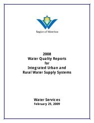
August 26, 2011Sam ZiemannPage 6 of 12Reference: Fluid Transient Analysis for Strange Street Raw Water Supply System – Draft TechnicalMemorandumthe Data Collection section. The model was then opened in Bentley Systems HAMMERtransient analysis software and saved.The following assumptions were made during model construction:• The Multiple Point pump type pump definitions provided in the model fromthe Kitchener Office were used in the transient analysis model. Thesedefinitions are based upon the pump curves.• A water elevation of 333.79 m was used as the downstream boundarycondition for the Strange Street Reservoir.• The following Hazen-Williams C-factors were used for watermains in themodel: 100-120 for CI and DI watermains; and 150 was used for high densitypolyethylene (HDPE) and PVC watermains.• Flow control valves were added to the model at each well to limit flows to therates provided in Table 1.• No air valves are installed on the Strange Street Water Supply System thathave the ability to allow air to enter the pipeline to prevent vacuumconditions.• Since the timing of well starts and stops was not provided, it was assumedwell starts occurred over a 5-second period and pump stops wereinstantaneous and the same as a power failure induced pump trip. Theseassumptions were made to estimate worst-case transient conditions withinthe raw water supply system.• The future raw water storage tank will be constructed at the Strange StreetReservoir site.• Operating pressure information was not provided. Therefore, the model wascalibrated based upon flow using the capacities within Table 1.Results for the water supply system indicate hydraulic conditions within the systemtransition from pressure to gravity flow approximately 1,150 m west of the GlaskowStreet/Belmont Avenue intersection. Therefore, a pressure sustaining valve was addedat the location where flow conditions transition from full pipe/pressurized flow to partiallyfull pipe/gravity flow to maintain pressurized flow upstream of this point. As shown inFigures 1 and 2, the slope of portions of the raw water supply system mains exceedsthe slope of the hydraulic grade. This will result in gravity flow conditions along portionsof the raw water supply system downstream of the pressure sustaining valve location.Figures 1 and 2 illustrate the hydraulic grade calculated by the model along the raw

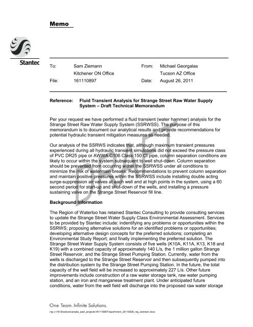
August 26, 2011Sam ZiemannPage 7 of 12Reference: Fluid Transient Analysis for Strange Street Raw Water Supply System – Draft TechnicalMemorandumwater supply system piping from the K18/K19 Well House to the Strange StreetReservoir.The point where flow conditions transition from full pipe/pressurized flow to partially fullpipe/gravity flow conditions represents a boundary condition for the fluid transient modelas the model is limited to performing computations under pressure flow conditions.In order to perform the existing conditions transient analysis for the SSRWSS, themodel piping was truncated in the model at the location of the pressure sustaining valveand a Discharge to Atmosphere element was added to represent this transition point.The model was then rerun.Existing System Transient AnalysisThe first stage of the transient analysis was to develop and analyze scenarios of theexisting system for worst case transients. The following operational scenarios thatwould result in a change in steady-state flows were evaluated:1. Simultaneous shut-down of all wells due to power failure2. Sudden shut-down of one well (K18)3. Start-up of one well (K18) during normal operations (5 s start-up)Scenario 1 – Simultaneous shut-down of all wells due to power failureScenario 1 modeled a power failure (pump trip) event with all of the well pumps inoperation. The sudden shut-down of the well pumps induced a negative pressure wavethat propagated downstream. Figures 3a and 3b, which illustrate the pressure and headexperienced along the raw water supply system piping from the K18/K19 Well House tothe end of the truncated model, indicate that full vacuum conditions and columnseparation (macro-cavitation) occur along almost the entire segment of watermain.Macro-cavitation conditions occur when the negative pressures in the watermain dropor fall to the vapour pressure of the fluid. This phenomenon, which is known as columnseparation, results in the formation of large pockets of vapour within the watermain.Later, on the returning upsurge, these vapour pockets can collapse violently and thehigh pressure caused by the two liquid columns coming together can cause watermainruptures or damage to system components. Column separation places undesirablestresses on piping systems and should be avoided whenever possible.Scenario 2 – Well K18 Sudden Shut-downScenario 2 modeled a sudden shut-down event with one well in operation. This scenariois intended to represent normal operating conditions and assumes the wells within thesystem are shut-down one at a time. For this scenario the shut-down of Well K18 wasevaluated. Well K18 was chosen because it is the greatest distance away from the end

August 26, 2011Sam ZiemannPage 8 of 12Reference: Fluid Transient Analysis for Strange Street Raw Water Supply System – Draft TechnicalMemorandumof the truncated model. Results for Scenario 2, which are shown in Figures 4a and 4b,are similar to those of Scenario 1 and indicate full vacuum conditions occur over most ofthe segment of watermain from the K18/K19 Well House to the end of the truncatedmodel.Model results show that the maximum transient pressures within the pipeline during apump shut-down can exceed steady-state pressure conditions by as much as 710 kPa.Results also indicate it is likely the pressures within portions of the raw water supplysystem reach atmospheric or subatmospheric conditions when there are no wells inoperation and that a segment of the system may empty into the Strange StreetReservoir subsequent to shut-down of all the wells. This is because the high waterelevation of the Strange Street Reservoir is below the well head elevations. It isundesirable to allow pressures within the raw water supply system to reach atmosphericconditions as it increases the potential for contamination of the watermains and canallow air to enter the raw water supply system. If air within the raw water supply systemis not managed correctly, air binding could occur and reduce the watermain carryingcapacity by causing an increase in head loss.Scenario 3 – Well K18 Start-up: 5 secondsFor this scenario start-up of Well K18 over a 5-second period was modeled. Figures 5aand 5b show the head and pressure experienced along the raw water supply systempiping from the K18/K19 Well House to the end of the truncated model for a 5-secondwell pump start-up. Results indicate the maximum pressures experienced within the rawwater supply system can exceed steady-state pressures by approximately 330 kPa.Pressure Control AlternativesFor the second stage of the transient analysis effective means of controlling thepressure fluctuations calculated for Scenarios 1-3 during pump start-ups, shut-downs,and power failures were examined.Controlling Pressures During Power Failure Induced Pump TripsPower failure induced pump trips cause a sudden drop in discharge header pressure asthe pumps suddenly de-energize. The installation of air valves within the raw watersupply system to allow air to enter the system can help prevent column separation.Scenario 4 modeled the same power failure (pump trip) event with all of the wellspumps in operation as Scenario 1 except that air valves were input along the watermainand at each well in an attempt to prevent macro-cavitation conditions from occurring.Double acting surge-suppression air valves with 50 mm inlet and 7.93 mm outlet orificeswere used to model the air valves. The valves were sized based upon manufacturer’spublished information. Figures 6a and 6b, which illustrates the pressure and headexperienced along the raw water supply system piping from the K18/K19 Well House to

August 26, 2011Sam ZiemannPage 9 of 12Reference: Fluid Transient Analysis for Strange Street Raw Water Supply System – Draft TechnicalMemorandumthe end of the truncated model, indicates that, although negative pressures within theraw water supply system piping occur immediately downstream of the K18/K19 WellHouse and at the downstream end of the model, full vacuum conditions and columnseparation (macro-cavitation) are avoided. The double acting surge-suppression airvalves input along the raw water supply system piping within the model are the reasonmacro-cavitation conditions are avoided.Model results show that the maximum transient pressures within the watermains forScenario 4 do not exceed steady-state pressure conditions by more than approximately80 kPa. Model results also show that the modeled air valve size is sufficient to preventcolumn separation from occurring in the raw water supply system piping.Controlling Pump Shut-down PressuresPump shut-down pressures should be such that negative pressures within the watersupply system are avoided. For normal pump shut-down this can be accomplished withthe use of variable speed drives, soft-stop controls, pump control valves, or acombination of these.Scenario 5 was developed to minimize the occurrence of negative pressures within theraw water supply system subsequent to a pump shut-down and assumed the soft-startat the wells were programmed with a ramp down time of 60 seconds. Figures 7a and7b, which display the Scenario 5 results, demonstrate that shutting the pumps downover a 60-second period essentially eliminates negatives pressures within the raw watersupply system.Controlling Pump Start-up PressuresScenario 6 models the use of soft-start controls to start-up Well K18 over a 30-secondperiod. Figures 8a and 8b, which display the Scenario 6 results, show that the pressureincrease within the water supply system from the K18/K19 Well House to the end of thetruncated model is limited to approximately 135 kPa above steady-state conditions.Maintaining Raw Water Supply System Pressure during Normal Operating ConditionsPressures within the raw water supply system should remain above atmosphericpressure during normal start-up and shut-down of the wells. This can be accomplishedwith the use of control valves and/or a reservoir placed at the location where flowconditions transition from full pipe/pressurized flow to partially full pipe/gravity flow tomaintain pressurized flow conditions downstream of these points.Scenario 7 models the installation of a control valve, specifically a pressure sustainingvalve, on the Strange Street Reservoir fill line to maintain positive pressure within theraw water supply system subsequent to shut-down of Well K18 over a period of 60

August 26, 2011Sam ZiemannPage 10 of 12Reference: Fluid Transient Analysis for Strange Street Raw Water Supply System – Draft TechnicalMemorandumseconds. Although it is unlikely the pressure sustaining valve could react fast enoughduring a rapid transient event such as a power failure, the pressure sustaining valve canhelp maintain positive pressures within the raw water supply system during a controlledshut-down of the wells. The pressure sustaining valve is set to maintain a hydraulicgrade of 365 m within the watermain upstream of the Strange Street Reservoir. Thissetting should result in a minimum pressure of 140 kPa within the raw water supplysystem during steady-state conditions.Scenario 7 results, which are shown in Figures 9a and 9b, indicate positive pressuresare maintained within the raw water delivery system during the shut-down of Well K18over a period of 60 seconds.Anticipated Future ConditionsAnticipated future improvements to the Strange Street Water Supply System include:• Replacement of an existing 300 mm main from the Glasgow Street/Knell Driveintersection near Well K11A to the Gage Avenue/Belmont Avenue intersectionwith 450 mm PVC DR25 pipe.• The addition of a new well(s) and replacement wells to increase the raw watersupply system capacity to 227 L/s.• Construction of a raw water storage tank to receive discharge from the wellsprior to providing iron and manganese water treatment and discharging thetreated water into the Strange Street Reservoir.As indicated previously in Table 1, it is anticipated that the new well(s) will have acapacity of 40 L/s. Scenario 8 was developed to model a power failure (pump trip) eventwith all of the wells pumps in operation at a total capacity of 227 L/s. For this scenario, anew 40 L/s capacity well was placed in the vicinity of the Well K18/K19 Well House.This scenario assumes the air valves referenced in Scenario 4 are installed.Figures 10a and 10b display the results of Scenario 8 and indicate full vacuumconditions and column separation (macro-cavitation) are avoided.Conclusions and RecommendationsThe following conclusions and recommendations are summarized regarding thetransient analysis of the Strange Street Water Supply System:Conclusions• Transient analysis results indicate it is likely that column separation occurswithin the SSRWS subsequent to a power failure induced pump trip with all wells

August 26, 2011Sam ZiemannPage 11 of 12Reference: Fluid Transient Analysis for Strange Street Raw Water Supply System – Draft TechnicalMemorandumin operation as well as subsequent to a sudden shut-down with one well inoperation.• Model results show the maximum pressures experienced along the raw watersupply system piping from the K18/K19 Well House to the end of the truncatedmodel can exceed steady-state pressures by approximately 330 kPa for a 5-second well pump start-up.• Model results indicate the maximum transient pressures experienced during allhydraulic transient simulations on the SSRWS did not exceed the pressure class(1,140 kPa) of PVC DR25 pipe or AWWA C106 Class 150 CI pipe.• Model results indicate the installation of double acting surge-suppression airvalves at each well and at high points within the SSRWSS prevents full vacuumconditions and column separation (macro-cavitation) from occurring within thesystem subsequent to power failure (pump trip) event with all of the wells pumpsin operation.• Model results indicate full vacuum conditions and column separation (macrocavitation)within the raw water supply system are avoided if the well pumps areshut-down over a period of 60 seconds.• Model results indicate the pressure increase within the water supply systemfrom the K18/K19 Well House to the end of the truncated model is limited toapproximately 135 kPa above steady-state conditions during pump start-up ifsoft-start controls are used to start-up the wells over a 30-second period.Recommendations• Confirm the type of air valves installed at each of the wells.• Determine existing soft-start and soft-stop ramp times for the wells.• Use a 60 second period for start-up and shut-down of the well pumps and do notstart-up or shut-down more than one well pump at a time.• Consider installing 100 mm combination air valves with 7.93 mm orifices on thedischarge piping at each of the wells and at high points along the raw watersupply system to prevent macro-cavitation.• Marco-cavitation should be prevented from occurring within the SSRWS underall conditions to minimize the risk of watermain breaks.

August 26, 2011Sam ZiemannPage 12 of 12Reference: Fluid Transient Analysis for Strange Street Raw Water Supply System – Draft TechnicalMemorandum• Transient control strategies for the SSRWS should focus on applications thatprotect against downsurge and column separation, as well as pump controlalternatives to reduce the transient pressure envelope during pump start-up andshut-down.• Consider installation of a pressure sustaining valve on the Strange StreetReservoir fill line with a hydraulic grade setting of 365 m to maintain positivepressure within the raw water supply system during normal well start-up andshut-down.• Conduct field testing to confirm the effectiveness of the selected control strategyat limiting pressures within the raw water supply system.We trust the above analysis provides the information needed to assist in thedevelopment of alternative design concepts. If you should have any questions, pleasedo not hesitate to contact us.STANTEC CONSULTING SERVICES INC.Michael Georgalas, PEAssociate, Environmental Infrastructuremichael.georgalas@stantec.comAttachment: Figures 1-10c. John Take

Elevation (m)K18/K19 Well House to Strange St. Reservoir - Current Conditions394392390388386384382380Pressure Flow OnlyPressure and Gravity Flow378376374372370368366364362360358356354352350348346344Strange Street Reservoir342340338336Pressure Sustaining Valve334332330328326K18/K19 Well House32432232002004006008001,0001,2001,4001,600Distance (m)1,8002,0002,2002,4002,6002,8003,0003,200Existing - All Wells ON - Hydraulic GradeExisting - All Wells ON - ElevationClient/ProjectStrange Street Water Supply SystemTransient AnalysisFigure No.1TitleExisting Water Supply SystemHydraulic Profile Steady-state Conditions

Pressure (kPa)K18/K19 Well House to Strange St. Reservoir - Current Conditions740720700680Pressure Flow OnlyPressure and Gravity Flow660640620600580560540520500480460440420400380360340320300280260240220200180Strange Street Reservoir16014012010080604020K18/K19 Well HouseSustaining Valve`Pressure0-2002004006008001,0001,2001,4001,600Distance (m)1,8002,0002,2002,4002,6002,8003,0003,200Existing - All Wells ON - PressureClient/ProjectStrange Street Water Supply SystemTransient AnalysisFigure No.2TitleExisting Water Supply SystemPressure Steady-state Conditions

Figure 3a – Existing ConditionsPump Shutdown – Wells K10A, K11, K13, K18, & K19 (136 l/s): Power Failure (Head Envelope)Figure 3b – Existing ConditionsPump Shutdown – Wells K10A, K11, K13, K18, & K19 (136 l/s): Power Failure (Pressure Envelope)Head Legend:Pipeline ElevationInit. Conditions HeadMax. Transient HeadMin. Transient HeadVapour HeadPressure Legend:Transmission MainInit. Conditions Press.Max. Transient Press.Min. Transient Press.Vapour Press.Client / ProjectFigure No.TitleStrange Street Water Supply System.Transient Analysis3a & 3bExisting ConditionsScenario 1: Shutdown All Wells (power failure)

Figure 4a – Existing ConditionsPump Shutdown – Well K18 (53 l/s): Power Failure (Head Envelope)Figure 4b – Existing ConditionsPump Shutdown – Wells K18 (53 l/s): Power Failure (Pressure Envelope)Head Legend:Pipeline ElevationInit. Conditions HeadMax. Transient HeadMin. Transient HeadVapour HeadPressure Legend:Transmission MainInit. Conditions Press.Max. Transient Press.Min. Transient Press.Vapour Press.Client / ProjectFigure No.TitleStrange Street Water Supply System.Transient Analysis4a & 4bExisting ConditionsScenario 2: Shutdown Well K18

Figure 5a – Existing ConditionsWell K18 (53 l/s) Pump Start-up: 5 Seconds (Head Envelope)Figure 5b – Existing ConditionsWells K18 (53 l/s) Pump Start-up: 5 Seconds (Pressure Envelope)Head Legend:Pipeline ElevationInit. Conditions HeadMax. Transient HeadMin. Transient HeadVapour HeadPressure Legend:Transmission MainInit. Conditions Press.Max. Transient Press.Min. Transient Press.Vapour Press.Client / ProjectFigure No.TitleStrange Street Water Supply System.Transient Analysis5a & 5bExisting ConditionsScenario 3: Start-up Well K18 (5 Seconds)

Figure 6a – Existing System w/Combination Air ValvesPump Shutdown – Wells K10A, K11, K13, K18, & K19 (136 l/s): Power Failure (Head Envelope)Figure 6b – Existing System w/Combination Air ValvesPump Shutdown – Wells K10A, K11, K13, K18, & K19 (136 l/s): Power Failure (Pressure Envelope)Head Legend:Pipeline ElevationInit. Conditions HeadMax. Transient HeadMin. Transient HeadVapour HeadPressure Legend:Transmission MainInit. Conditions Press.Max. Transient Press.Min. Transient Press.Vapour Press.Client / ProjectFigure No.TitleStrange Street Water Supply System.Transient Analysis6a & 6bExisting System w/Air ValvesScenario 4: Shutdown All Wells (power failure)

Figure 7a – Existing ConditionsWell K18 (53 l/s) Pump Shutdown: 60 Seconds (Head Envelope)Figure 7b – Existing ConditionsWell K18 (53 l/s) Pump Shutdown: 60 Seconds (Pressure Envelope)Head Legend:Pipeline ElevationInit. Conditions HeadMax. Transient HeadMin. Transient HeadVapour HeadPressure Legend:Transmission MainInit. Conditions Press.Max. Transient Press.Min. Transient Press.Vapour Press.Client / ProjectFigure No.TitleStrange Street Water Supply System.Transient Analysis7a & 7bExisting ConditionsScenario 5: Shutdown Well K18 (60 seconds)

Figure 8a – Existing ConditionsWell K18 (53 l/s) Pump Start-up: 30 Seconds (Head Envelope)Figure 8b – Existing ConditionsWells K18 (53 l/s) Pump Start-up: 30 Seconds (Pressure Envelope)Head Legend:Pipeline ElevationInit. Conditions HeadMax. Transient HeadMin. Transient HeadVapour HeadPressure Legend:Transmission MainInit. Conditions Press.Max. Transient Press.Min. Transient Press.Vapour Press.Client / ProjectFigure No.TitleStrange Street Water Supply System.Transient Analysis8a & 8bExisting ConditionsScenario 6: Start-up Well K18 (30 Seconds)

Figure 9a – Existing System w/Combination Air Valves and Pressure Sustaining ValveWell K18 (53 l/s) Pump Shutdown: 60 Seconds (Head Envelope)Figure 9b – Existing System w/Combination Air Valves and Pressure Sustaining ValveWell K18 (53 l/s) Pump Shutdown: 60 Seconds (Pressure Envelope)Head Legend:Pipeline ElevationInit. Conditions HeadMax. Transient HeadMin. Transient HeadVapour HeadPressure Legend:Transmission MainInit. Conditions Press.Max. Transient Press.Min. Transient Press.Vapour Press.Client / ProjectFigure No.TitleStrange Street Water Supply System.Transient Analysis9a & 9bExisting System w/Air Valves and PSVScenario 7: Shutdown Well K18 (60 seconds)

Figure 10a – Future System w/Combination Air Valves and Pressure Sustaining ValvePump Shutdown – Wells K10A, K11, K13, K18, & K19 (136 l/s): Power Failure (Head Envelope)Figure 10b – Future System w/Combination Air Valves and Pressure Sustaining ValvePump Shutdown – Wells K10A, K11, K13, K18, & K19 (136 l/s): Power Failure (Pressure Envelope)Head Legend:Pipeline ElevationInit. Conditions HeadMax. Transient HeadMin. Transient HeadVapour HeadPressure Legend:Transmission MainInit. Conditions Press.Max. Transient Press.Min. Transient Press.Vapour Press.Client / ProjectFigure No.TitleStrange Street Water Supply System.Transient Analysis10a & 10bFuture System w/Air Valves and PSVScenario 8: Shutdown All Wells (power failure)

APPENDIX DTreatability Information

MD-80 CATALYTIC MEDIAIRON, MANGANESE, ARSENIC AND HYDROGEN SULFIDE REMOVALPRODUCT OVERVIEWMD-80 by Napier-Reid Limited is a high-performance catalytic oxidative media. The media isused in water treatment applications for iron, manganese and hydrogen sulfide removal. It isalso used in removal of other heavy metals such as lead and arsenic. It is a media that utilizesan oxidation, adsorption and filtration process similar to greensand and Birm, but at a muchhigher level of performance and capacity.Because of MD-80 media’s high content of manganese dioxide (MnO2) it provides a highercatalysis and adsorption capability than other media. Manganese dioxide works as a catalystto accelerate the oxidation reaction between the oxidants (dissolved oxygen or other oxidantsinjected) and the soluble iron, manganese and sulfide. The oxidized form will precipitate andthen be filtered out by the media bed. Iron and manganese that are not oxidized becomecatalytically precipitated and adsorbed on the media .The adsorbed iron, manganese are expelled during backwash. Any trapped solid form of iron,manganese and sulfur particles are also flushed out of the filter during backwash cycle. It isvery important to make sure that the media receives a thorough backwash to break loose andremove the contaminant particles and keep the bed clean to maintain its high capacity. Toensure a good performance daily backwash is recommended. Air scour will help theregeneration of the MD-80 media especially when there is no continuous addition of oxidants.Although MD-80 can be used without chemicals for most low-level contaminants the additionof oxidants, such as chlorine, ozone, hydrogen peroxide and potassium permanganate greatlyenhances the performance and extends the service life of the MD-80 media.MD-80 outperforms most of other media for iron, manganese and sulfide removal. It is alsorecommended as a pre-treatment step for ion-exchange softener, RO system and GACcontactor.If there is presence of arsenic and iron in the raw water, iron will be oxidized to iron oxide andarsenic will be adsorbed onto iron oxide and removed from the water together with iron. Thiscan either be a stand-alone process or as a pre-treatment step prior to other arsenic removalprocess based on adsorption principle to prolong the service life of the adsorption media.Ferric chloride solution can be added to increase the iron to arsenic ratio if necessary.MD-80 is capable of removing virtually unlimited amounts of the above contaminants, buttends to work better in some geographic areas than others depending on the levels of TDS orHeme Iron (organics) in the local water supplies. If you have had success in the past withgreensand, Birm®, Pyrolox, or Filox-R, then MD-80 will work for you using the sameparameters.10 Alden Road, Unit 2Markham, Ontario L3R 2S1, CanadaTel: (905) 475-1545 1-800-615-4406 Fax: (905) 475-2021E-mail: info@napier-reid.com / Website: www.napier-reid.com

TECHNICAL SPECIFICATIONSPHYSICAL PROPERTIESColour:Grey - BlackActive Ingredients: 75% - 85%Physical Form: GranularMesh Size: 20 x 40Bulk Density: 110 lbs / ft 3Specific Gravity: 4Taste and Odour: NoneLife Expectancy: Virtually unlimited forlow contaminantconditionsSHIPPING INFOMATIONPackaging:Pallets:Heavy-duty paper bag.55 or 1100 lbs per bag.40 Bags/Pallet.2300 lbs per palletOPERATING CONDITIONSService Flow Rate: 5 – 10 gpm/ft 2Freeboard: 30% - 40%Backwash Rate: 20 – 25 gpm/ft 2@ 60°FBed Depth: 20” to 35”Terminal Headloss: 10 psi Max.Backwash Frequency: 24 – 48 hrsPH Range: 5.0 – 9.0CERTIFICATIONThe MD-80 media is certifiedto NSF/ANSI Standard 61 andis suitable for potable waterapplications.SERVICE FLOW PRESSURE DROPBACKWASH BED EXPANSION10 Alden Road, Unit 2Markham, Ontario L3R 2S1, CanadaTel: (905) 475-1545 1-800-615-4406 Fax: (905) 475-2021E-mail: info@napier-reid.com / Website: www.napier-reid.com

NR – Pressure FiltersHorizontal and Vertical Pressure FiltersforMunicipal and Industrial Water treatmentWater & Wastewater Treatment

Napier-Reid Ltd.Pressure FiltersNR - Pressure Filter - Process DescriptionNapier Reid’s pressure filtration systems are designed to carry out filtration in closed vessel underpressurized condition. As NR Pressure Filters have high filtration rate and ability to operate at higherpressure drop compared to gravity filters and the footprint is relatively smaller compared toconventional gravity filters.In NR – Pressure Filters, the incoming raw water is distributed over the filtration area of the filterthrough our unique well designed flow distribution system. The water filters down through the differentlayers of the filter bed. The filtration media mechanically strains out dirt, suspended solids, sediment,algae, bacteria, microscopic worms, cryptosporidium and asbestos, colour, odour, precipitates of iron/manganese and other impurities.The filter bed is designed to capture and hold the suspended solids and impurities throughout thedepth of the filter bed (and not just at the surface layer), hence increasing the solids holding capacity.Also the filter bed and internals are designed to prevent channeling and media upset. The capability ofNR pressure filters to operate at higher terminal headlosses and higher solids holding capacity resultsin longer filter runs and a reduced backwash water requirement.The filtered water is evenly collectedover the filtration area by our uniquewater collection system that preventschanneling and short circuiting.When the differential pressure acrossthe filter increases beyond a presetvalue, the filter bed is backwashed toremove the entrapped impurities inthe filter media bed and return thefilter to its original filtration capacity.NR filters are equipped with airscouring system and efficientbackwash water distribution systemfor effective backwash.NR - Pressure Filtration SkidOPG Lennox Power Generation StationBath, OntarioDesign Flow Rate: 197 m 3 per day2

Napier-Reid Ltd.Pressure FiltersSalient Features of NR - Pressure Filters• High filtration rate up to 10 gpm/ft 2 (24 m/hr)• High solids holding capacity, and ability tooperate at high pressure loss, resulting inlonger filter runs and reduced backwashwater requirement as little as 2% of plant flow.• High flexibility in mode of operation.• Degree of automation can be provided asper client’s requirement, from completelymanual to fully automatic complete withautomatic control valves, PLC / SCADAcontrol package, and control panel.• Available in vertical and horizontalconfiguration.• Supplied with suitable media: dual bed, multimedia bed, GAC or MD-80 catalytic media foriron and manganese, arsenic, H 2S removal.• Well designed feed water distribution system.• Efficient under-drain collection / backwashdistribution system for minimal pressure dropand proper backwashing.• Efficient backwash and air scour system.• Package design and multi-tank configurationavailable. System can be supplied skidmounted, completely assembled, or loose forfield assembly on concrete pads.• Material of construction - Carbon steel orFiberglass reinforced polyester (FRP),designed for 150 psig pressure.NR - Pressure GAC TowerSouth Chatam, OntarioDesign Flow of each tower:7600 m 3 per day• All CS vessels are designed and fabricatedin accordance with ASME code. The vesselcan be ASME “U” stamped if required.• Carbon steel pressure vessel, interior NSFapproved epoxy lined suitable for potablewater service and prime exterior finished.• All carbon steel vessels provided with liftinglugs and appropriate size manways.NR - Horizontal FiltersIsashi, Lagos, Nigeria• Smaller footprint compared to other systems.• High degree of automation leads to reducedoperator attention and lower O&M cost.Process designers of Napier Reid have over 300 years of cumulative experience.3

Napier-Reid Ltd.Pressure FiltersNR - Pressure Filter ApplicationsNR Pressure Filters are widely used for filtrationof suspended solids and other impurities from:Municipal WaterMunicipal WastewaterSurface waterGround waterIndustrial wastewaterNR – Pressure Filters forFe-Mn RemovalInnerkip, Ontario, CanadaDesign Flow 1296 m 3 per dayNR - Pressure Filtration skidc/w automatic valves & control panelThamesford WTP, OntarioDesign Flow 5520 m 3 per dayAbout Napier - ReidOver 50 years of excellence in water & wastewater treatmentNapier-Reid is located in the greater Toronto area in the Province of Ontario,Canada. We supply engineering services and process equipment for water andwastewater treatment.We have the technology, resources and experience to design, manufacture andimplement innovative water and wastewater treatment solutions worldwide. Wehave completed over 3000 projects since our inception in 1950. This stands as atestament of our ongoing commitment of providing the highest quality service,products and after sales support in the industry. Our capabilities includeengineering, manufacturing, installation and field support. We have in-housepersonnel for complete mechanical, electrical and instrumentation process andcontrol system design. As a manufacturer, our designs focus on cost-effectivesolutions, simplicity of installation and ease of maintenance.10 Alden Road, Unit 2Markham, Ontario L3R 2S1CanadaTel: (905) 475 1545Fax: (905) 475 2021E-mail: info@napier-reid.comwww.napier-reid.comNapier-Reid has developed an excellent team with many years of experience. Wehave a well-deserved reputation for innovation, service and integrity. A significantportion of Napier-Reid’s business is now exported to regions such as theCaribbean, Central America, South America, Middle East, Eastern Europe, Africa,and Asia. Some of these projects are financed by Canadian government orInternational financing institutes. As a Canadian manufacturer, we are eligible forCanadian governmental funding and EDC export credit. We have the capability tohandle a large range of projects, from engineering, equipment supply, installation,start-up, to turnkey projects. Let Napier-Reid be your single solution for water andwastewater purification.©2007, Napier-Reid Ltd. All rights reserved. All product names and brands mentioned here are registered trademark of Napier-Reid or their respective companies.Product’s specifications are subject to change without any prior notice.4

APPENDIX EHydrogeological Assessment

HYDROGEOLOGICALASSESSMENTSTRANGE STREET WATERSUPPLY CLASS EA UPDATEREGIONAL MUNICIPALITY OFWATERLOOPrepared for:Regional Municipality of Waterloo150 Frederick Street, 7th FloorKitchener ON N2G 4J3Prepared by:Stantec Consulting Ltd.49 Frederick StreetKitchener ON N2H 6M7161110897March 2012

HYDROGEOLOGICAL ASSESSMENTSTRANGE STREET WATER SUPPLY CLASS EA UPDATEREGIONAL MUNICIPALITY OF WATERLOOTable of Contents1.0 INTRODUCTION .............................................................................................................. 1.12.0 BACKGROUND REVIEW ................................................................................................. 2.12.1 PHYSIOGRAPHY AND TOPOGRAPHY ........................................................................... 2.12.2 SURFACE WATER FEATURES AND ENVIRONMENTAL AREAS .................................. 2.12.3 GEOLOGY AND HYDROGEOLOGY ................................................................................ 2.12.3.1 Hydrostratigraphy ............................................................................................... 2.32.3.2 Local and Regional Hydrogeology ...................................................................... 2.62.4 WELL FIELD DESCRIPTION ............................................................................................ 2.72.5 AQUIFER ASSESSMENT ................................................................................................. 2.82.6 WELL PERFORMANCE.................................................................................................... 2.92.6.1 Production Well K10A ........................................................................................ 2.92.6.2 Production Well K11A ...................................................................................... 2.102.6.3 Production Well K13 ......................................................................................... 2.102.6.4 Former Production Well K15............................................................................. 2.102.6.5 Production Well K18 ......................................................................................... 2.102.6.6 Production Well K19 ......................................................................................... 2.112.7 WATER QUALITY ........................................................................................................... 2.112.7.1 Chloride and Sodium ........................................................................................ 2.112.7.2 Iron ................................................................................................................... 2.122.7.3 Manganese ...................................................................................................... 2.122.7.4 Sulphate ........................................................................................................... 2.122.7.5 Nitrate .............................................................................................................. 2.132.7.6 Volatile Organic Compounds ............................................................................ 2.133.0 METHODOLOGY FOR TEST WELL ................................................................................ 3.13.1 IDENTIFICATION OF TEST DRILLING LOCATIONS ....................................................... 3.13.2 RESIDENTIAL NOTIFICATION ......................................................................................... 3.13.3 MONITORING WELL INSTALLATION .............................................................................. 3.23.4 TEST WELL INSTALLATION ............................................................................................ 3.33.5 GEODETIC SURVEY ........................................................................................................ 3.33.6 PERMIT TO TAKE WATER APPLICATION ...................................................................... 3.33.7 PERFORMANCE TESTING .............................................................................................. 3.33.8 GROUNDWATER LEVEL MONITORING ......................................................................... 3.43.9 GROUNDWATER SAMPLING AND TESTING ................................................................. 3.54.0 RESULTS FOR TEST WELL ............................................................................................ 4.14.1 TEST WELL DRILLING LOCATIONS ............................................................................... 4.14.2 GEOLOGY ........................................................................................................................ 4.14.3 WELL CONSTRUCTION................................................................................................... 4.34.4 GROUNDWATER DISCHARGE ....................................................................................... 4.4hls v:\01609\active\161110897_strange_st\planning\report\final hydrogeo assessment\final\fnl_rpt_120319.docxi

HYDROGEOLOGICAL ASSESSMENTSTRANGE STREET WATER SUPPLY CLASS EA UPDATEREGIONAL MUNICIPALITY OF WATERLOOTable of Contents4.5 VARIABLE RATE PUMPING TEST .................................................................................. 4.44.6 CONSTANT RATE PUMPING TEST ................................................................................ 4.54.7 ESTIMATE OF AQUIFER PARAMETERS ........................................................................ 4.74.8 THEORETICAL WELL YIELD ........................................................................................... 4.84.9 WATER QUALITY ............................................................................................................. 4.85.0 CONCLUSIONS ............................................................................................................... 5.16.0 RECOMMENDATIONS ..................................................................................................... 6.17.0 REFERENCES ................................................................................................................. 7.1iihls v:\01609\active\161110897_strange_st\planning\report\final hydrogeo assessment\final\fnl_rpt_120319.docx

HYDROGEOLOGICAL ASSESSMENTSTRANGE STREET WATER SUPPLY CLASS EA UPDATEREGIONAL MUNICIPALITY OF WATERLOOTable of ContentsList of AppendicesAppendix AAppendix BAppendix CAppendix DAppendix EAppendix FAppendix GAppendix HAppendix IAppendix JAppendix KAppendix LFiguresTablesLotowater Technical Services Inc. ReportsTechnical Memorandum A1 – Strange Street Well Field Water QualityAssessmentTechnical Memorandum A2 – Identification of Preferred Test Drilling LocationsResidential Notification LetterTest Well Log, Monitoring Well Logs and Water Well RecordsPermit to Take Water No. 1160-8FQK6SAQTESOLV TM AnalysisLaboratory Certificates of AnalysisLetter of Compliance and SOP for Drilling Fluid Release to Sanitary SewerRisk Assessment – Discharge to Storm Water Sewer During PerformanceTestinghls v:\01609\active\161110897_strange_st\planning\report\final hydrogeo assessment\final\fnl_rpt_120319.docxiii

HYDROGEOLOGICAL ASSESSMENTSTRANGE STREET WATER SUPPLY CLASS EA UPDATEREGIONAL MUNICIPALITY OF WATERLOOTable of ContentsList of FiguresAppendix AFigure 1Figure 2Figure 3Figure 4Figure 5Figure 6Figure 7Figure 8Figure 9Well Field LocationSurficial Geology and TopographyConceptual Cross-Section of the Waterloo MoraineCross-Section A-A’Historical Production Well Water Quality DataPotential Test Drilling TargetsSite Plan – Gzowski ParkK-SS-TW1-11 Performance Test ResultsPerformance Test Response HydrographsList of TablesAppendix BTable 1Table 2Table 3Production and Monitoring Well Construction DetailsGroundwater Quality Analytical ResultsCalculation of Potential Well Capacityivhls v:\01609\active\161110897_strange_st\planning\report\final hydrogeo assessment\final\fnl_rpt_120319.docx

HYDROGEOLOGICAL ASSESSMENTSTRANGE STREET WATER SUPPLY CLASS EA UPDATEREGIONAL MUNICIPALITY OF WATERLOO1.0 IntroductionThe Regional Municipality of Waterloo (Region) is undertaking the Strange Street Water SupplySystem Class Environmental Assessment (Class EA) Update. The primary objective of thisstudy is to update the Class EA and Preliminary Design completed by the Region in 2001, withthe first component of this study focusing on groundwater investigations. Since 2001, a varietyof work has been conducted in the Strange Street Well Field (Figure 1), including wellrehabilitation and assessment efforts, and the installation of two (2) new production wells(Production Wells K11A and K19) (Stantec, 2005; Burnside, 2007). In addition, recent work hasbeen completed by the Ontario Geological Survey (OGS) (Bajc and Shirota, 2007) and Stantec(2009) consisting of a detailed review of the hydrostratigraphy of the Waterloo Moraine andbedrock units throughout the Region, which resulted in a detailed update of thehydrostratigraphy within the Strange Street Well Field (Stantec, 2009).The Region retained Stantec Consulting Ltd. (Stantec) to complete the hydrogeologicalassessment related to the Class EA Update which was broken down into the followingobjectives:• Assess historical and current water quality data and production well performance data withinthe Strange Street Well Field supply aquifer;• Review and assess existing groundwater data to identify potential test drilling locations;• Construction of monitoring wells and test wells at up to two (2) preferred test drillinglocations; and• Performance testing and groundwater sampling of the new test well(s).This report has been organized into seven sections, including this introduction (Section 1.0).Section 2.0 provides a background summary of the well field geology and hydrogeology.Methodologies are presented in Section 3.0 with results presented in Section 4.0. Conclusionsand recommendations are presented in Sections 5.0 and 6.0, respectively with reportreferences presented in Section 7.0.All figures and tables referenced throughout the report are presented in Appendices A and B,respectively. Lotowater Technical Services Inc. (Lotowater) well performance reports areprovided in Appendix C. Technical Memorandums A1 and A2 are presented in Appendix D andE, respectively. The residential notification letter is presented in Appendix F. Test well,monitoring well logs, and water well records are presented in Appendix G. A copy of the PTTWand application package is provided in Appendix H. Appendices I though L presentAQTESOLV TM Analysis, Laboratory Certificates of Analysis, letter of compliance, and the riskassessment related to discharge water quality, respectively.hls v:\01609\active\161110897_strange_st\planning\report\final hydrogeo assessment\final\fnl_rpt_120319.docx 1.1

HYDROGEOLOGICAL ASSESSMENTSTRANGE STREET WATER SUPPLY CLASS EA UPDATEREGIONAL MUNICIPALITY OF WATERLOO2.0 Background Review2.1 PHYSIOGRAPHY AND TOPOGRAPHYThe Strange Street Well Field is located along the eastern flank of the physiographic regionreferred to by Chapman and Putnam (1984) as the Waterloo Moraine. The Moraine is orientedin a north south direction with ground surface topography decreasing from a high of over400 metres (m) above mean sea level (AMSL) within the core areas of the Waterloo Morainenear St. Agatha, to a low of approximately 300 m AMSL at the Grand River. Locally, within thevicinity of the Strange Street Well Field, the ground surface topography ranges fromapproximately 370 m AMSL to 340 m AMSL (Figure 2) with a general slope to the east.2.2 SURFACE WATER FEATURES AND ENVIRONMENTAL AREASThe topographic high, corresponding to the core of the Waterloo Moraine, creates a regionalsurface water divide that diverts surface water to the Nith River in the west and the Grand Riverin the east. Locally, a topographic divide exists to the south of the Strange Street Well Fieldwith surface water flow on the northern portion of the divide draining to Maple Hills Creek whichis part of Laurel Creek (Figure 2). To the south of the divide, surface water flow is towards theHenry Sturm and Detweiler Greenways that are part of the Upper Schneider Creek Watershed(Figure 2).Maple Hills Creek flows to the north where it joins with Clair Creek near Waterloo Park. Thedrainage basin for Maple Hills Creek has been developed for residential use, and as a resulthas been altered to some degree, particularly for the older development areas (Figure 2). Thecreeks to the south of the divide have been substantially altered to allow for urban drainagewithin the development areas. The Henry Sturm Greenway has been channelized through theconstruction of concrete lined urban drainage channels (Figure 2). Upstream ofFischer-Hallman Road, the Henry Sturm Greenway has been incorporated into a morenaturalized setting, with riparian vegetation and buffers. The Detweiler Greenway is a tributaryto the Sandrock Greenway, and runs parallel to Highland Road (Figure 2). The DetweilerGreenway has been incorporated into a naturalized corridor upstream of Highland Road.Several on-line stormwater management facilities exist along Detweiler Greenway for waterquality control, and to mitigate downstream flooding impacts.Locally, there are no Areas of National and Scientific Interest (ANSI), Environmentally SensitivePolicy Areas (ESPA), or provincially significant wetlands within the Study Area.2.3 GEOLOGY AND HYDROGEOLOGYThe Quaternary geology of the Study Area has been studied extensively and is discussed byKarrow (1993). The Waterloo Moraine is a kame moraine formed during an interlobate positionbetween ice lobes extending from the Ontario-Erie, Huron, and Georgian Bay Basins. Ahls v:\01609\active\161110897_strange_st\planning\report\final hydrogeo assessment\final\fnl_rpt_120319.docx 2.1

HYDROGEOLOGICAL ASSESSMENTSTRANGE STREET WATER SUPPLY CLASS EA UPDATEREGIONAL MUNICIPALITY OF WATERLOOBackground ReviewMarch 19, 2012conceptual cross section of the Waterloo Moraine is presented on Figure 3. Numerousadvances and retreats of these ice lobes during the Wisconsin glaciation have resulted in acomplex deposit of ice-contact and glacial outwash sands and gravels separated by silt- andclay-rich tills. Along the flanks of the Moraine, meltwaters resulting from the retreat of glacial iceeroded and cut through the various till and sand and gravel units. The resulting glaciofluvialsediments are typically stratified and sorted to varying degrees.Previous interpretations of the geology and resulting hydrostratigraphy of the Waterloo Morainerelied mainly on the correlation of individual till units across the moraine (Karrow, 1993). Thiswas generally found to be a reasonable approach in the core areas of the moraine where sheetlike till units exist; however, it did not provide a detailed understanding of the sand and gravelunits that were previously mapped as ice-contact stratified drift. In 2002, the Ontario GeologicalSurvey (OGS) embarked on a three year project to produce 3-dimensional mapping of thesurficial deposits within the Region. The methodology and interpretation of the surficial depositsare detailed in Bajc and Shirota (2007).Karrow (1993) referred to the first till units deposited in the area as the Pre-Catfish Creek Tills.These till units are interpreted to be mid- to early-Wisconsinan in age and include the CanningTill and several other unnamed tills. The Canning Till is one of the more continuous andrecognizable Pre-Catfish Creek Tills, although this till is not encountered at all locations withinthe Moraine. The Canning Till is described by Karrow (1993) at its type section near Canningas a nearly pebble-free, purplish, silty clay or clayey silt till. The unnamed Pre-Catfish Tillswithin the Study Area are generally hard, stony silt to clayey silt tills, similar in appearance to theCatfish Creek Till.The Catfish Creek Till is the next till sheet deposited by a major glacial advance from the northto northeast that covered all of southern Ontario. As a result, the Catfish Creek Till isinterpreted to be the first major stratigraphic marker throughout the Waterloo Moraine. TheCatfish Creek Till is an extremely dense, stony, sandy silt to silt till and is commonly referred toas “hardpan” by many water well drillers.One of the most important till units throughout the Waterloo Moraine is the Maryhill Till. TheMaryhill Till is a dense, dark brown, clayey silt to silty clay till and represents the main aquitardunit that protects the deeper aquifer systems utilized by a number of municipal well fields,including the Greenbrook Well Field. Karrow (1993) has interpreted the Maryhill Till asover-riding the sands of the Waterloo Moraine; however, this interpretation has been refined byPaloschi (1993) and more recently by the work of Bajc and Shirota (2007), which have identifiedthree separate ice advances that have resulted in an Upper, Middle, and Lower Maryhill Tillwithin the core area of the Waterloo Moraine.The next two tills deposited after the Maryhill Till within the general Study Area are the Tavistockand Port Stanley Tills. The Tavistock Till was deposited by ice advances from the2.2 hls v:\01609\active\161110897_strange_st\planning\report\final hydrogeo assessment\final\fnl_rpt_120319.docx

HYDROGEOLOGICAL ASSESSMENTSTRANGE STREET WATER SUPPLY CLASS EA UPDATEREGIONAL MUNICIPALITY OF WATERLOOBackground ReviewMarch 19, 2012Huron-Georgian Bay ice lobes and is mainly restricted to the western flanks of the WaterlooMoraine. The Tavistock Till is a dark brown clayey silt till, similar in composition to the MaryhillTill, and may correspond to the isolated till units capping the Waterloo Moraine that are referredto by Karrow (1993) as the Maryhill Till. If this is the case, then the Tavistock Till may havebeen deposited within the Study Area along the eastern flank of the Moraine. The Port StanleyTill is similar in age to the Tavistock Till and was deposited by ice advancing from theErie-Ontario ice lobe and is mainly restricted to the eastern flanks of the Waterloo Morainewhich includes the study area. The Port Stanley Till is a sandy silt to silty sand till and isoccasionally stony.Figure 2 presents the surficial Quaternary geology for the general Study Area based oncompiled mapping by OGS (2003). The surficial geology within the Study Area consists ofpredominantly glaciofluvial sandy and gravelly deposits with occasional pockets of stone-poor,sandy silt to silty sand till and clay to silt textured till. Along the major surface water bodiesincluding the Grand River, Strasburg Creek and Schneider Creek, modern day alluvial depositshave been identified at surface (Figure 2).The Paleozoic bedrock geology beneath the Study Area consists of the Salina and GuelphFormations. The Salina Formation consists of interbedded brown dolostone and grey to greenshale with lenses of gypsum and anhydrite. Typically, groundwater extracted from the SalinaFormation within the Region is of poor quality due to high concentrations of calcium andsulphate resulting from the dissolution of gypsum and anhydrite minerals. The GuelphFormation is a cream-coloured crystalline dolostone and represents an important supply aquiferto the northeast in the area of Guelph, and to the east in the City of Cambridge. The contactbetween the Salina and Guelph Formations is interpreted to be slightly west of the Study Area.2.3.1 HydrostratigraphyA comprehensive review of the geology and hydrogeology of the Waterloo Moraine wasundertaken as part of the Study of the Hydrogeology of the Waterloo Moraine in 1995(Terraqua, 1995). As part of this work, a conceptual hydrogeologic model for the moraine wasdeveloped, consisting of three overburden aquifers (Aquifers 1, 2, 3), separated by fouraquitards (Aquitards 1, 2, 3, 4). The upper portion of the bedrock aquifer in the area wasclassified as the fourth aquifer unit (Aquifer 4).Recent work by Bajc and Shirota (2007) resulted in a conceptual geological model for theRegion that consists of an aquifer/aquitard sequence with 19 layers. Many of these layers arefound only locally. Nine layers were identified to be the most regionally significant, andgenerally correspond with those presented by Terraqua (1995). In the naming convention usedby Bajc and Shirota (2007) aquitard units are identified with AT followed by a letter and number(e.g., ATB1), whereas aquifers are identified with AF followed by a letter and number(e.g., AFB1).hls v:\01609\active\161110897_strange_st\planning\report\final hydrogeo assessment\final\fnl_rpt_120319.docx 2.3

HYDROGEOLOGICAL ASSESSMENTSTRANGE STREET WATER SUPPLY CLASS EA UPDATEREGIONAL MUNICIPALITY OF WATERLOOBackground ReviewMarch 19, 2012The following presents details of the conceptual model based on Terraqua (1995) and Bajc andShirota (2007). The local hydrostratigraphic model is summarized in Figure 4, which is an eastto west cross section through the Strange Street Well Field:Aquitard 1 (ATB1):Aquitard 1 consists of low permeability, spatially discontinuous, surficial till units foundpredominantly along the flanks of the Waterloo Moraine, which are readily identified in surficialgeology mapping. Along the western flank of the moraine, Aquitard 1 corresponds to theMornington, Stratford and Tavistock Tills; whereas along the eastern flank of the Moraine, thisunit corresponds to the Upper Maryhill and Port Stanley Tills (Bajc and Shirota, 2007). Withinthe Strange Street Well Field, ATB1 is identified as a silt to clayey till, with a maximum thicknessof 15 m. It is found at higher elevations, and where the ground surface elevation drops, the unitis not typically present, or is thinner as is evident in Figure 4.Aquifer 1(AFB1/ATB2/AFB2):Aquifer 1 represents the main water supply aquifer in the core areas of the Waterloo Moraine.The Strange Street Well Field is completed in Aquifer 1 and represents the most eastern wellfield completed in this unit. Depending on the depositional environment, the composition ofAquifer 1 can vary from a layered silt and fine sand to coarse sand and gravel. Aquifer 1 isinterpreted to be bisected by the middle Maryhill Till (ATB2), effectively separating Aquifer 1 intotwo units, AFB1 and AFB2. Within the Strange Street Well Field, AFB1 consists of a range offine to medium sands, and is not continuous. It is most prominent at higher elevations, andtherefore when the ground surface elevation drops off to the east, AFB1 is observed to thin orpinch out (Stantec, 2009).Within the Strange Street Well Field, ATB2 is found to be a discontinuous, silty to clayey till unit.This unit is typically thicker towards the core area of the Waterloo Moraine, and it either thins oris not present in the eastern portion of the Strange Street Well Field (Figure 4). The presence ofATB2 may locally impact the vertical movement of groundwater through Aquifer 1 whereverpresent, however, on a large scale, Aquifer 1 is interpreted to behave as a single system.All of the current Production Wells (K10A, K11, K13, K18, and K19) within the Strange StreetWell Field are interpreted to be screened within AFB2. This layer typically ranges in thicknessfrom 0 to 40 m, with an average thickness of about 10 m and is typically not present below anelevation of 310 m AMSL. It is predominantly defined by fine and medium sand, silt, and gravelbased on continuous core logging data. As was the case for AFB1, AFB2 appears to pinch outlocally to the east (Figure 4) and to the south (Stantec, 2009). This interpretation is furtheraugmented by the fact that former Production Wells in the east (K15, K16 and K17), as well aswells in the nearby Greenbrook Well Field, were all completed in lower aquifer systems,presumably because Aquifer 1 was not sufficiently thick to support a municipal well.2.4 hls v:\01609\active\161110897_strange_st\planning\report\final hydrogeo assessment\final\fnl_rpt_120319.docx

HYDROGEOLOGICAL ASSESSMENTSTRANGE STREET WATER SUPPLY CLASS EA UPDATEREGIONAL MUNICIPALITY OF WATERLOOBackground ReviewMarch 19, 2012Aquitard 2 (ATB3):Aquitard 2 (ATB3) corresponds to the lower Maryhill Till and represents one of the primaryregional hydrostratigraphic units. The till has been broken down into a Middle and LowerMaryhill Till by Bajc and Shirota (2007). Along the flanks of the moraine the Maryhill Till is oftenfound to be discontinuous, or has been re-worked and re-deposited as glaciofluvial sediments.Within the Strange Street Well Field, it was found to be continuous and range in thickness from5 m to 25 m (Stantec, 2009). It is defined as a clayey silt to silty clay till, physically separatingthe upper aquifer system (Aquifer 1) from the lower aquifer systems (Aquifers 2 and 3)(Figure 4).Aquifer 2 (AFB3/AFC1):Aquifer 2 corresponds to the lower Waterloo Moraine Stratified Sediments (AFB3) and CatfishCreek Drift (AFC1) as referred to by Karrow (1993), and when present is found belowAquitard 2, mainly along the eastern flank of the Moraine. This unit consists of stratified gravels,sands, or silts and is of very limited extent. As a result Aquifer 2 was rarely identified within theStrange Street Well Field (Stantec, 2009).Aquitard 3 (ATC1/ATC2):Aquitard 3 corresponds to the Catfish Creek Till. Bajc and Shirota (2007) divided this unit intoan upper (ATC1) and lower aquitard (ATC2), with Aquifer 2 (AFC1) found occasionally betweenthe two units. This unit is nearly continuous throughout the Region and together withAquitard 2, forms the main stratigraphic marker units within the Moraine. The texture of this unitis a stony, silty to sandy till, and is often referred to as “hardpan” in well logs. Within theStrange Street Well Field, ATC1 is interpreted to be continuous, with ATC2 rarely beingidentified, which could partially be a function of the limited number of deep boreholes in the area(Figure 4). Often, Aquitard 3 directly underlies Aquitard 2, likely providing an effective confininglayer between Aquifer 1 and Aquifers 3 and 4.Aquifer 3 (AFD1/AFF1):Aquifer 3 is spatially discontinuous throughout much of the core areas of the Waterloo Moraine,and is found either directly overlying bedrock or overlying Aquitard 4. AFD1 likely correspondsto sands and gravel re-worked from Catfish Creek and Pre-Catfish Creek Tills, and representsthe main supply aquifer in the Cities of Kitchener and Waterloo with the Greenbrook, Parkway,and William Street Well Fields all completed in this unit (Bajc and Shirota, 2007). AFF1 isinterpreted to correspond to the sand and gravel units typically found beneath Aquitard 4,directly overlying bedrock. This unit is discontinuous throughout the Region, and where presentis hydraulically connected with the upper weathered portion of the bedrock aquifer.Due to the limited information available from high reliability, deep borehole logs, interpretation ofthe geologic units below ATC1 is difficult (Stantec, 2009). Often, because not all these lowerunits were identifiable, distinguishing between similar aquifer units (i.e. AFC1, AFD1, and AFF1)hls v:\01609\active\161110897_strange_st\planning\report\final hydrogeo assessment\final\fnl_rpt_120319.docx 2.5

HYDROGEOLOGICAL ASSESSMENTSTRANGE STREET WATER SUPPLY CLASS EA UPDATEREGIONAL MUNICIPALITY OF WATERLOOBackground ReviewMarch 19, 2012presented some challenges, and therefore it was difficult to determine the horizontal extent andcontinuity of each of these layers.Aquitard 4 (ATE1/ATG1):Aquitard 4 corresponds to the Pre-Catfish Creek Till and Canning Drift. This unit is foundprimarily in the central, northern and western areas of the Region, and along the Nith River inthe west and southwest. As a result Aquitard 4 units were typically found to be discontinuousthroughout the Strange Street Well Field (Stantec, 2009), however, similar to the unitsassociated with Aquifer 3, delineation of these units was challenging as a result of the lack ofdeep boreholes.Bedrock:The Paleozoic bedrock geology beneath the Strange Street Well Field consists of the Salinaand Guelph Formations (OGS, 1991). The Salina Formation consists of interbedded dolostoneand shale with lenses of gypsum and anhydrite. Typically, groundwater extracted from theSalina Formation within the Region is of poor quality due to high concentrations of calcium andsulphide resulting from the dissolution of gypsum and anhydrite minerals. The GuelphFormation is a dolostone and represents an important aquifer to the east of Kitchener-Waterloonear Guelph, and to the south in the City of Cambridge. The contact between the Salina andGuelph Formations is interpreted to be present in the eastern portion of the Strange Street WellField (OGS, 1991).2.3.2 Local and Regional HydrogeologyThe most recent delineations of regional groundwater flow within Aquifer 1 and Aquifer 3, werepresented by AquaResource (2009). The general regional groundwater flow direction withinAquifers 1 and 3 is from west to east from the core areas of the Waterloo Moraine, including inthe Strange Street Well Field. Groundwater levels within Aquifer 1 decrease from a high ofapproximately 350 m AMSL near the core area of the Waterloo Moraine, to a low of310 m AMSL to the east of the well field. Groundwater flow within Aquifer 1 is predominantlyhorizontal and results from regional recharge within the core areas of the Waterloo Moraine,near St. Agatha, and local recharge where Aquitard 1 is absent and Aquifer 1 is exposed atground surface. Where Aquitard 2 is absent, a hydraulic connection between Aquifer 1 andAquifers 2/3 may exist, resulting in vertical flow and recharge to the deeper aquifer units.The hydrogeology of the Strange Street Well Field has been characterized by numerousstudies, the most prominent of which include:• K11 Aquifer Test (IWS, 1942)• TW3-74 (near K18) Aquifer Test (IWS, 1974)• K18 Aquifer Test (IWS, 1975)• K10A Aquifer Test (IWS, 1982);2.6 hls v:\01609\active\161110897_strange_st\planning\report\final hydrogeo assessment\final\fnl_rpt_120319.docx

HYDROGEOLOGICAL ASSESSMENTSTRANGE STREET WATER SUPPLY CLASS EA UPDATEREGIONAL MUNICIPALITY OF WATERLOOBackground ReviewMarch 19, 2012• Aquifer Shutdown Test (Terraqua, 1995);• Kitchener Westside Pumping Test (Stantec, 2000);• K19 Aquifer Test (Stantec, 2005);• K11A Aquifer Test (Burnside, 2007);• Mapping of Shallow and Deep Potentiometric Surfaces (AquaResource, 2009); and• Tier 3 Water Budget and Water Quality Risk Assessment (Stantec, 2009).Groundwater flow within the Strange Street Well Field follows the general regional trendsdescribed above, with the predominant flow direction within Aquifer 1 being from west to east.Groundwater flow under pumping and non-pumping conditions was recently investigated and asummary of all previous reports can be found within the Tier 3 Water Budget and Water QualityRisk Assessment Report (Stantec, 2009).The recharge source area for the Strange Street Well Field was evaluated in Terraqua (1995).Terraqua (1995) concluded that the water captured by the well field is recharged locally.2.4 WELL FIELD DESCRIPTIONThe Strange Street Well Field is located within the northwest portion of the City of Kitchener andis generally spread out over an area of approximately 1.0 km 2 . The well field is divided into twogeneral areas. Production Wells K11A, K13, K18 and K19 are located in the western portion ofthe well field, in the vicinity of the Westmount Golf & Country Club (Figure 1). With theexception of the golf course, which is zoned as open space, land use in this area ispredominantly residential. Production Well K10A is located approximately 1 kilometer (km) tothe east on Gage Avenue within an area that is zoned as industrial/mixed use with residentialintermixed (Figure 1).The first wells for the Strange Street Well Field were constructed around 1910 and a pumpingstation was constructed in 1923. By the time the pumping station was constructed, there wereat least (9) wells installed to depths ranging from 14 m to 91 m below ground surface (BGS).The water supply for the Strange Street Well Field is currently obtained from Production WellsK10A, K11A, K13, K18 and K19. Production Wells K10, K11, K12, K14, K14A, K15, K16 andK17, which have been used historically for water supply purposes, have either been abandonedor replaced due to poor water quality or a decline in well yield. A detailed history of the StrangeStreet Well Field was documented in Stantec (2000). The following provides a brief summary ofthe status of the currently active production wells:• Production Well K10 was constructed following a test drilling program in 1935, and wasabandoned as a water supply source following the construction of Production Well K10A in1982. Production Well K10A is currently used as a water supply source;hls v:\01609\active\161110897_strange_st\planning\report\final hydrogeo assessment\final\fnl_rpt_120319.docx 2.7

HYDROGEOLOGICAL ASSESSMENTSTRANGE STREET WATER SUPPLY CLASS EA UPDATEREGIONAL MUNICIPALITY OF WATERLOOBackground ReviewMarch 19, 2012• Production Well K11 was constructed in 1942. Due to declines in well performance,Production Well K11 was replaced with Production Well K11A in 2007 (Burnside, 2007).Production Well K11A was commissioned in October 2011;• Production Well K13 was constructed in 1946 following the completion of a test drillingprogram on the former Bauer Farm property. Production Well K13 is currently used as awater supply source;• Production Well K18 was constructed in 1975 following the completion of a test drillingprogram on the Westmount Golf & Country Club in 1974. Production Well K18 is currentlyused as a water supply source for both the Region and as an irrigation source for theWestmount Golf & Country Club; and• Production Well K19 was constructed in 2005 on the Westmount Golf & Country Clubproperty following a test drilling program (Stantec, 2005) and is presently used as a watersupply source.A summary of the Production Well details are provided in Table 1. All of the existing ProductionWells are completed within Aquifer 1 (AFB2) at depths typically ranging from 17 m BGS to38 m BGS. Production Wells K10A, K11, K13 and K18/K19 were all constructed with adouble-walled gravel packed well screen.The Strange Street Well Field is governed by a single Permit To Take Water (3058-7JCLBY)that allows for combined pumping from Production Wells K10A, K11A, K13, K18 and K19 at amaximum pumping rate of 11,467 L/min and a maximum daily taking of 16,512.48 m 3 /day.2.5 AQUIFER ASSESSMENTThe Class EA hydrogeologic assessment completed in 2000 by Stantec included an evaluationof the sustainable yield of the aquifer within the Strange Street Well Field, identified locations forpotential new production wells, and confirmed water quality of production wells.Stantec (2000) evaluated the long-term aquifer yield based on the combined informationobtained from historical water level data, aquifer testing results, and the groundwater flowmodeling completed using the Waterloo Moraine Model. The data was used to assess thedrawdown under known pumping conditions and to complete theoretical calculations of aquiferresponse and the required recharge to balance pumping. The long-term sustainable yield ofAquifer 1 (ATB1) in the K10A, K11, K13, and K18 area was estimated to be 100 L/s to 120 L/s(Stantec, 2000).Stantec (2000) also reviewed groundwater quality results which were compared to the ODWS.Manganese, hardness, total dissolved solids, and occasionally iron were the main parametersdetected within the production wells above applicable ODWS. These parameters are either2.8 hls v:\01609\active\161110897_strange_st\planning\report\final hydrogeo assessment\final\fnl_rpt_120319.docx

HYDROGEOLOGICAL ASSESSMENTSTRANGE STREET WATER SUPPLY CLASS EA UPDATEREGIONAL MUNICIPALITY OF WATERLOOBackground ReviewMarch 19, 2012aesthetic objectives or operational guidelines under the ODWS and are not related to healthconcerns. No volatile organic compounds were detected at concentrations at or evenapproaching the ODWS. In general, the water quality at Production Wells K12 and K17 waspoor in comparison to wells K10A, K11, K13, and K18. Chloride represented the mainparameter of concern with respect to long term water quality, mainly because treatment ofchloride is not currently practical.2.6 WELL PERFORMANCEThe most recent well performance information for each municipal well is provided below. Someof this work was completed as part of this Class EA Update and the rest was completed as partof the Region’s routine Well Maintenance Program. Copies of the most recent completedreports for Production Wells K10A, K15 and K19 are provided in Appendix C.2.6.1 Production Well K10AWell performance evaluation at Production Well K10A was completed by Lotowater fromNovember 2008 to May 2009 (Lotowater, 2009). The key outcomes of this evaluation included:• The structural integrity of the well was restored through the installation of a new stainlesssteel liner as well as upgrades to the wellhead and discharge connections; and• In an effort to improve well performance, an acid-based cleaning solution was injected andsurged into the well, but no significant increase in well performance was achieved. Resultingwell capacity was 58% of the as-constructed capacity, and it was thought that the wellshould be able to produce 12 L/s to 15 L/s, where historically the well could produce 25 L/sto 30 L/s.Additional well rehabilitation and testing was subsequently conducted by Lotowater in January,2011 (Lotowater, 2011a) (Appendix C). The key outcomes of this testing program included:• A multi-phase physical and chemical rehabilitation program was undertaken which includedchemical injection of a polyphosphate solution, an acid-based cleaning solution, and areducing agent, all aimed at removing buildup on the well screen in an attempt to restorewell performance. The combination of these treatments proved effective, with the acidtreatment providing the greatest improvement in well performance;• Following treatment, the well was restored to approximately 77% of its as-constructedperformance levels. The well should now be capable of pumping up to its permitted rate of26.5 L/s, however, it is limited by the pump, which is capable of operating up to a maximumflow rate of approximately 20 L/s; andhls v:\01609\active\161110897_strange_st\planning\report\final hydrogeo assessment\final\fnl_rpt_120319.docx 2.9

HYDROGEOLOGICAL ASSESSMENTSTRANGE STREET WATER SUPPLY CLASS EA UPDATEREGIONAL MUNICIPALITY OF WATERLOOBackground ReviewMarch 19, 2012• Lotowater recommended performing ongoing monitoring and service in order to maintain thewell performance, and installing a larger pump in order to meet the well’s permitted capacity.2.6.2 Production Well K11AThe as-constructed performance at Production Well K11A was completed in March, 2007 byLotowater and is documented in Burnside (2007). The specific capacity of the well followinginstallation was 6.8 L/s/m of drawdown at a pumping rate of 60 L/s. In March 2010, theperformance of the well was checked again and found to be 6.3 L/s/m of drawdown at apumping rate of 60 L/s, which was 93% of the as-constructed performance. A video inspectionindicated that the casing and screen were in good condition with no build-up or blockagesobserved.Production Well K11A was commissioned in October 2011.2.6.3 Production Well K13Production Well K13 was most recently evaluated in October and November of 2009 byLotowater (Lotowater, 2010a). During this evaluation, it was noted that well performancedecreased significantly since construction in 1946, and the well is currently performing atapproximately 21% of its as-constructed capacity. The well is currently capable of producing12 L/s.2.6.4 Former Production Well K15Production Well K15 has not been used for municipal drinking water supply since the 1990’sand most recently was operated by the City of Kitchener for non-potable water purposes.Production Well K15 was recently evaluated by Lotowater in February of 2011 (Lotowater,2011b) (Appendix C). During this investigation, the submersible pump was found to be in poorcondition and was permanently removed. A video inspection showed a substantial amount ofbuild-up on the well casing. Foreign objects consisting of scrap wire and a 1 m section of pipewere also found within the well. Based on these findings it was determined that the foreignobjects should be removed from the well, and the well should be abandoned using acombination of bentonite grout and concrete.2.6.5 Production Well K18Production Well K18 was most recently evaluated by Lotowater (2010) and the well capacitywas near as-constructed performance. A significant amount of build-up was noted on thescreen and was removed using a combination of mechanical brushing and a weak acid solution.The pump was de-staged to allow pumping to the Strange St. Reservoir and is available to bebrought back online when needed.2.10 hls v:\01609\active\161110897_strange_st\planning\report\final hydrogeo assessment\final\fnl_rpt_120319.docx

HYDROGEOLOGICAL ASSESSMENTSTRANGE STREET WATER SUPPLY CLASS EA UPDATEREGIONAL MUNICIPALITY OF WATERLOOBackground ReviewMarch 19, 20122.6.6 Production Well K19Production Well K19 was evaluated by International Water Supply (IWS) from December 2007to February 2008 (IWS, 2009). At the time, the specific capacity of the well was 2.2 L/s/m ofdrawdown at a pumping rate of 43 L/s, compared to the as-constructed specific capacity of3.2 L/s/m of drawdown at a pumping rate of 51.3 L/s, with an as-constructed pumping rate inexcess of 60 L/s. Sand production was also noted at pumping rates above 38 L/s.Rehabilitation efforts performed by IWS were unsuccessful in restoring lost capacity.As a result of the IWS evaluation, additional diagnostic testing was recommended (Stantec,2010a). Lotowater completed pre-rehabilitation step-testing on March 9, 2010 (Appendix C),and determined that the well’s performance was approximately 65% of the as-constructedperformance (Lotowater, 2010b). Extensive well rehabilitation was performed, andpost-rehabilitation testing determined that the well’s performance had improved to within 80% ofthe original as-constructed performance, and would be capable of operating at up to 52 L/s.The well is currently back in service.2.7 WATER QUALITYAvailable historical and current water quality trends from production wells and monitoring wellswithin the Strange Street Well Field were reviewed and compared to the Ontario Drinking WaterStandards (ODWS). The results are documented in Technical Memorandum A1 – StrangeStreet Well Field Water Quality Assessment which is provided in Appendix D for reference. Keyparameters of interest within the aquifer included chloride, sodium, iron, manganese, sulphateand nitrate. Consistent with other production wells throughout the Region, all monitoring andproduction wells exhibit elevated hardness. Volatile organic compounds were not detectedwithin any of the wells sampled during the 2010 field program. A summary of the water qualityparameters of interest for the Strange Street Well Field are summarized below, with datasummarized in Figure 5.2.7.1 Chloride and SodiumAn increasing trend in chloride has been noted in all the existing and former Production Wellswithin the Strange Street Well Field (Figure 5). Chloride concentrations exceeding the ODWSAesthetic Objective (AO) of 250 milligrams per litre (mg/L) were observed at ProductionWell K10A with concentrations of chloride at Production Wells K11 and K13 less than 150 mg/L(Figure 5). A similar upward trend was noted in the concentration of sodium, suggesting thatwinter road salt activities are the likely source of the impacts. It also suggests that the watercaptured by the production wells may be recharging locally, particularly in the eastern end of thewell field. Water quality analysis at monitoring wells throughout the well field found elevatedchloride and sodium in select wells (Stantec, 2000; Appendix D).hls v:\01609\active\161110897_strange_st\planning\report\final hydrogeo assessment\final\fnl_rpt_120319.docx 2.11

HYDROGEOLOGICAL ASSESSMENTSTRANGE STREET WATER SUPPLY CLASS EA UPDATEREGIONAL MUNICIPALITY OF WATERLOOBackground ReviewMarch 19, 2012With some exceptions, the monitoring and production wells on the western edge of the well field(such as K13 and K11) typically have lower concentrations of chloride and sodium than thosewells further east (such as K12 and K17). In particular, wells east of Westmount Road tend toexhibit elevated sodium and chloride.2.7.2 IronIron concentrations found within production wells have varied historically, but are typically belowthe ODWS AO of 0.3 mg/L (Figure 5). Iron levels within raw water obtained from ProductionWell K10/K10A have been the most variable, with occasional spikes in the data resulting inexceedances of the ODWS AO. Water quality results obtained from monitoring wells in the2010 sampling event found elevated iron concentrations in all wells (Appendix D). During the1999 sampling event (Stantec, 2000), the ODWS AO was exceeded in monitoring wells near allthe currently active production wells. Elevated iron is naturally found in groundwater extractedfrom this aquifer, and is not the result of anthropogenic activity.2.7.3 ManganeseWithin the Strange Street Production Wells, manganese has historically been near or above theODWS AO of 0.05 mg/L (Figure 5). A slight increasing trend was noted for all production wells,with Production Wells K10/K10A and K11 typically having the highest levels of manganese.Production Well K12 also exhibited elevated levels of manganese while in operation, typicallyabove 0.4 mg/L. Within monitoring wells sampled as part of the 2010 monitoring program(Appendix D), elevated manganese was observed to be above the ODWS AO in all monitoringwells located east of Production Wells K18 and K19. Elevated manganese is naturally found ingroundwater extracted from this supply aquifer, and is not the result of anthropogenic activity.2.7.4 SulphateSulphate concentrations at Production Wells within the Strange Street Well Field have beenrelatively stable since monitoring began in the early 1980’s (Figure 5). At all Production Wells,with the exception of one exceedance by Production Well K17 in October of 1982, sulphatelevels have remained below the ODWS AO of 500 mg/L. All currently active Production Wellshave been consistently below 200 mg/L since 1995.Sulphate concentrations of samples collected from monitoring wells within the study area werebelow the ODWS AO and did not exceed 100 mg/L, with the exception of SS13-99 (Figure 2),where sulphate was measured at 177 mg/L (Appendix D). The results are consistent withStantec (2000) where sulphate was not observed to be above the ODWS AO in any of themonitoring wells.2.12 hls v:\01609\active\161110897_strange_st\planning\report\final hydrogeo assessment\final\fnl_rpt_120319.docx

HYDROGEOLOGICAL ASSESSMENTSTRANGE STREET WATER SUPPLY CLASS EA UPDATEREGIONAL MUNICIPALITY OF WATERLOOBackground ReviewMarch 19, 20122.7.5 NitrateConcentrations for nitrate have remained well below the ODWS Maximum AcceptableConcentration (MAC) of 10 mg/L (Figure 5), with the exception of one occurrence at ProductionWell K11 in June of 1987 where nitrate concentrations reached 9.25 mg/L. Since 2000, levelsfor nitrate at all active Production Wells have remained below 1 mg/L. Nitrate concentrations inmonitoring wells were consistently either not detected or was found to be well below the ODWSMAC.2.7.6 Volatile Organic CompoundsUpon reviewing historical volatile organic compound water quality data for the production wells,the following parameters were observed on more than one occasion in the indicated productionwell:• 1,4 dioxane was detected twice between 2004 and 2007 in Production Well K10A;• Tetrachloroethylene was detected twice in 2004 and 2005 at Production Well K10A andseven (7) times at Production Well K12 between 1992 and 1999; and• Phenolics, styrene, trichloroethylene, 1,1,1-Trichloroethane and 1,1-Dichloroethane werehistorically detected at Production Wells K12 and K17, located on the eastern edge of thewell field.Based on the 2010 water quality samples collected from monitoring wells throughout theStrange Street Well Field, which were non-detect for all tested volatile organic compounds(VOCs) (Appendix D – Table 1), and considering that most detections of organic compoundshave been found from the eastern portion of the well field from former Production Wells K12 andK17, VOCs are not considered to be a concern to water quality at the Strange Street Well Field.hls v:\01609\active\161110897_strange_st\planning\report\final hydrogeo assessment\final\fnl_rpt_120319.docx 2.13

HYDROGEOLOGICAL ASSESSMENTSTRANGE STREET WATER SUPPLY CLASS EA UPDATEREGIONAL MUNICIPALITY OF WATERLOO3.0 Methodology for Test WellBased on the assessment of existing well performance, hydrogeologic conditions and waterquality throughout the Strange Street Well Field, the need for at least one additional productionwell was identified. The following section details the methodology regarding the site selection,installation and performance testing of an additional test well completed within the StrangeStreet Well Field.3.1 IDENTIFICATION OF TEST DRILLING LOCATIONSIn 2010, Stantec completed a background review of potential test well drilling locations whichwas documented in Technical Memorandum A2 (Appendix E). Accessible land within theStrange Street Well Field was identified as parcels of land that were either owned by the Regionor the City of Kitchener. A total of six (6) potential test drilling locations were identified within theStrange Street Well Field:• Knell Drive (between K11A andK13);• Strange Street Reservoir;• K17 Well Site;• K12 Well Site;• Gzowski Park (east of K13); and• Westmount golf and Country Club.The potential test drilling locations are shown on Figure 6 and were evaluated based onthree (3) criteria; water quantity, water quality and ease of system connection. A numericalvalue was assigned to each criterion to assist with prioritizing each test drilling location with thelowest score corresponding to a preferred drilling location and a high score corresponding to aless desirable drilling location.3.2 RESIDENTIAL NOTIFICATIONPrior to commencement of drilling activities, a residential notification letter was delivered onJanuary 14, 2011 to residents living on Rossford Crescent and Chopin Drive betweenWestmount Road West and Markwood Drive (Figure 7). These houses were located adjacentto Gzowski Park and the proposed test well drilling location. The houses are supplied withmunicipal water and therefore the potential for well interference was not an issue. The letterdetailed the timing of drilling activities and discussed the potential for disturbances during theinstallation of the well and subsequent testing. A copy of the notification letter is provided inAppendix F.hls v:\01609\active\161110897_strange_st\planning\report\final hydrogeo assessment\final\fnl_rpt_120319.docx 3.1

HYDROGEOLOGICAL ASSESSMENTSTRANGE STREET WATER SUPPLY CLASS EA UPDATEREGIONAL MUNICIPALITY OF WATERLOOMethodology for Test WellMarch 19, 20123.3 MONITORING WELL INSTALLATIONA monitoring well nest was constructed at the location of K-SS-OW1-11 (Figure 7). The wellnest consisted of three individual monitoring wells installed within the overburden. GerritsDrilling and Engineering Ltd. (Gerrits) was retained by the Region to complete the monitoringwell drilling.Aardvark Drilling Inc. (Aardvark) was retained by Gerrits to complete the monitoring well drillingat K-SS-OW1A-11 between January 24, 2011 and February 4, 2011. The monitoring well wasadvanced using a CME75 truck-mounted drill rig. The 123 mm diameter borehole wasadvanced to the top of bedrock (82.6 m BGS) using mud rotary drilling techniques with 85 mmdiameter PQ continuous core samples collected over the entire depth of the borehole.Gerrits completed the monitoring well drilling at K-SS-OW1B-11 and K-SS-OW1C-11 betweenFebruary 16, 2011 and February 18, 2011. The monitoring wells were advanced using aDR-12 air fluid rotary drill rig. The 152 mm diameter borehole was advanced to target depths of28.9 m BGS and 10.7 m BGS at K-SS-OW1B-11 and K-SS-OW1C-11, respectively, using airfluid rotary drilling techniques. Water was used as the drilling fluid. During advancement ofK-SS-OW1B-11, grab samples were collected at 1.52 m intervals over the entire depth of theborehole. Gerrits completed grain size analysis on samples collected from 18.3 m BGS to27.4 m BGS to determine the grain size which represents 50% of the retained material.The recovered soil cores from K-SS-OW1A-11 were placed into PVC splits 1.52 m in length andlabeled in accordance with the Region core logging protocol (Region, 2008). Soil samples wereclassified by Stantec personnel using the America Society for Testing and Materials (ASTM)guideline for visual-manual description and identification of soils. Logs were prepared for theborehole, containing descriptions (where relevant and possible) of soil type, texture, colour,structure, moisture content, and other observations. Once drilling was completed, the core wasdelivered to the Region’s core storage location at the Mannheim Treatment Plant Site.All monitoring wells were constructed in separate boreholes using 49 mm ID Schedule 80 PVCwell casing for the deep (A) and intermediate (B) boreholes and 51 mm ID schedule 40 PVCwell casing for the shallow (C) borehole. The wells were constructed with No. 10 Slot (0.01 inchslot) PVC well screens, 3.05 m in length. The annular space between the monitoring well andformation was backfilled with No. 2 silica sand surrounding the screens. At K-SS-OW1C-11 theremainder of the annular space was filled with Holeplug TM to prevent hydraulic connection withinthe borehole. At K-SS-OW1A-11 and K-SS-OW1B-11 a combination of Holeplug TM andbentonite grout was used to fill the remainder of the annular space above and below the wellscreens to prevent hydraulic connection within the borehole. Positive displacement methodswere used to place the bentonite grout. The surface seal at all three (3) monitoring wellsconsisted of cement to 0.4 m BGS. All wells were constructed with individual lockable steelprotective casings.3.2 hls v:\01609\active\161110897_strange_st\planning\report\final hydrogeo assessment\final\fnl_rpt_120319.docx

HYDROGEOLOGICAL ASSESSMENTSTRANGE STREET WATER SUPPLY CLASS EA UPDATEREGIONAL MUNICIPALITY OF WATERLOOMethodology for Test WellMarch 19, 2012Following installation, the respective drilling company developed the wells to removefine-grained material from around the screened interval. Well development was completed to asand-free state using hydraulic air lifting, with the water generated during developmentdischarged to an onsite holding tank then pumped to the sanitary sewer accessed through amanhole on Rossford Crescent under permit from the City of Kitchener (Figure 7).All monitoring wells constructed as part of this investigation were completed in accordance withOntario Regulation 903 (O. Reg. 903). Monitoring well installation details are summarized inTable 1 and presented on the borehole logs in Appendix G. A copy of the completed MOEWater Well Records for each monitoring well is included in Appendix G.3.4 TEST WELL INSTALLATIONGerrits constructed a 154 mm OD well (K-SS-TW1-11) adjacent to K-SS-OW1-11. Constructionof Test Well K-SS-TW1-11 using air rotary drilling techniques was completed fromMarch 1, 2011 to March 9, 2011. Stantec field staff observed the test well drilling andinstallation. Test well installation details are summarized in Table 1 and presented on theborehole log in Appendix G. A copy of the completed MOE Water Well Record is included inAppendix G. Details related to the design and construction of K-SS-TW1-11 and welldevelopment are provided in Section 4.3.3.5 GEODETIC SURVEYGround surface and top of casing elevations and spatial coordinates at MonitoringWells K-SS-OW1A/B/C-11, K-SS-OW13-99, and Test Well K-SS-TW-1-11 were measuredusing a total station GPS unit. Following completion, the accuracy of the survey wasdetermined to be ±0.020 m.3.6 PERMIT TO TAKE WATER APPLICATIONOn behalf of the Region, Stantec prepared and submitted an application for a Category 2 PTTWto conduct a 24 hour performance test (step and constant rate test) at Test Well K-SS-TW1-11.The permit commenced on May 1, 2011 and extended until March 31, 2012, allowingcontinuous pumping over a 7-day period, to provide flexibility in the testing schedule and toaccount for any unforeseen delays. The maximum permitted taking per day was 2,592,000 L(1,800 L/min). A copy of PTTW No. 1160-8FQK6S is provided in Appendix H.3.7 PERFORMANCE TESTINGA variable rate pumping test was completed at K-SS-TW1-11 prior to commencing a 24 hourconstant rate pumping test. The performance testing was designed to evaluate aquiferproperties and water supply potential. Both the variable rate and constant rate pumping testswere completed by Gerrits, under the supervision of Stantec staff.hls v:\01609\active\161110897_strange_st\planning\report\final hydrogeo assessment\final\fnl_rpt_120319.docx 3.3

HYDROGEOLOGICAL ASSESSMENTSTRANGE STREET WATER SUPPLY CLASS EA UPDATEREGIONAL MUNICIPALITY OF WATERLOOMethodology for Test WellMarch 19, 2012The performance testing was completed with a temporary 152 mm diameter submersible pumpinstalled at a depth of 17.8 m below the top of casing (BTOC). The electrical supply wasprovided by a portable generator. During the performance testing, a Rossum Sand Tester wasinstalled in-line to assess the sand content of the water. A flow meter was used to monitor thepumping rate during the performance testing, with the water generated during developmentdischarged to an onsite holding tank then pumped to the sanitary sewer accessed through amanhole on Rossford Crescent (Figure 7). During performance testing, the water generatedwas discharged directly to the nearby stormwater distribution system on Westmount Road(Figure 7).The variable rate pumping test was conducted at K-SS-TW1-11 on June 13, 2011. Four stepsat pumping rates of 5 L/s, 10 L/s, 15 L/s, and 20 L/s were completed at approximately 30 minuteintervals with no recovery between steps.The constant rate pumping test at K-SS-TW1-11 was initiated on June 13, 2011 at 14:20immediately following the final 30 minute step of the variable rate pumping test and continuedfor 24 hours at a rate of 20 L/s ending on June 14, 2011. Results of the performance testing arepresented in Figures 8 and 9.Aquifer parameters were determined using the software package AQTESOLV TM . The results ofthe aquifer testing analyses are presented in Section 4.7 and Appendix I.3.8 GROUNDWATER LEVEL MONITORINGGroundwater levels were monitored within Test Well K-SS-TW1-11 and nearby MonitoringWells K-SS-OW1A/B/C-11, K-SS-OW13-99, K13, STOW2-07 and K-SS-OW1-82 throughout thestudy and during the performance testing.Groundwater monitoring was completed using a combination of manual and automatedtechniques. Monitoring wells and the test well were instrumented with either Diver Loggers ® orSolinst ® LT Leveloggers ® . Loggers were set to record at 30 second, 1 minute or 5 minuteintervals. The loggers are not vented to the atmosphere and therefore record total pressure. Asa result, data obtained from the loggers were corrected for atmospheric pressure to obtain theactual height of water above the sensor. The atmospheric corrections were made using datacollected from a Solinst Barologger ® , which was located about 20 km southeast of the Site andwithin the Region. Downloading of the loggers was completed by Stantec personnel. Regionstaff were responsible for installing Diver Loggers ® at K13 and STOW2-07.Manual measurements were collected at all wells using a battery operated probe and calibratedtape. Water depths were recorded in m BTOC. Gerrits collected manual water levelmeasurements at K-SS-OW1A/B/C-11 and K-SS-TW1-11 during the performance testing.3.4 hls v:\01609\active\161110897_strange_st\planning\report\final hydrogeo assessment\final\fnl_rpt_120319.docx

HYDROGEOLOGICAL ASSESSMENTSTRANGE STREET WATER SUPPLY CLASS EA UPDATEREGIONAL MUNICIPALITY OF WATERLOOMethodology for Test WellMarch 19, 2012Water level data collected during the performance testing are presented on hydrographs foreach monitored location in Figures 8 and 9.3.9 GROUNDWATER SAMPLING AND TESTINGGroundwater from K-SS-TW1-11 was sampled on March 9, 2011 at the end of welldevelopment (~8 hours), on June 13, 2011, 1.5 hours after the commencement of theperformance testing, and on June 14, 2011 at the end of the performance testing. All sampleswere analyzed for general chemistry, DOC, nutrients, metals, and inorganic parameters. Thesample collected on June 14, 2011 was also analysed for volatile organic compounds (VOCs),and microbiology parameters. None of the raw water samples were filtered and thereforeresults represent total concentrations.The samples were collected from the discharge hose and placed directly into appropriatelaboratory supplied sample containers. Samples were placed in coolers with ice and deliveredto Maxxam Analytics Inc. (Maxxam) under chain-of-custody documentation. The analyticalresults are summarized in Table 2 and compared to the ODWS. Appendix J contains a copy ofthe Laboratory Certificates of Analysis and chain-of-custody forms.hls v:\01609\active\161110897_strange_st\planning\report\final hydrogeo assessment\final\fnl_rpt_120319.docx 3.5

HYDROGEOLOGICAL ASSESSMENTSTRANGE STREET WATER SUPPLY CLASS EA UPDATEREGIONAL MUNICIPALITY OF WATERLOO4.0 Results for Test Well4.1 TEST WELL DRILLING LOCATIONSIn 2010, Stantec completed a background review and identified two (2) preferred test drillinglocations, Gzowski Park (TW3) and the Westmount Golf and Country Club (TW4) (Figure 6).The preferred test drilling locations were identified using a number of criteria including, potentialwell capacity, thickness of the target aquifer, potential water quality threats, proximity to existingwater supply infrastructure, and site access. Results of the test site selection were documentedin Technical Memorandum A2 (Appendix E).Both preferred test drilling locations scored high on water quantity and ease of connection to theexisting infrastructure, with a moderate score for water quality due to select parameterselevated above the ODWS which would be dealt with through the implementation of anupgraded treatment system.Based on the results of Technical Memorandum A2 (Appendix E), one (1) 127 mm diameter testwell, TW1-11 (Figure 1) was constructed and tested at preferred drilling location Gzowski Park.There was no additional test well installation completed at the second preferred drilling location,Westmount Golf and Country Club, due to issues with Site access.It should be noted that preferred test well drilling location Knell Drive (Between K11A and K13)scored highest based on the criterion and was previously identified in the initial Class EA as apreferred test drilling location. However, with the recent construction of K11A, and futurepotential rehabilitation/replacement of K13, installing a third production well in this area toprovide firm water capacity was no longer warranted.4.2 GEOLOGYIn support of construction of Test Well K-SS-TW1-11, an initial borehole was advanced to thetop of bedrock (81.9 m BGS) using continuous coring techniques. The initial pilot hole wasdrilled to the top of bedrock so that the entire overburden sequence could be evaluated. Thisapproach also addressed the data gap identified in the Tier 3 Water Budget and Water QuantityRisk Assessment (Stantec, 2009) that additional high quality deep overburden data was neededin the Strange Street Well Field area. The initial borehole was completed as monitoringwell K-SS-OW1A-11. The interpreted log for K-SS-OW1A-11 is included in Appendix G. Thefollowing is a summary of the geology encountered:AFB1 (Aquifer 1):A surficial layer of topsoil, underlain by clayey silt and sand to344.12 m AMSL (1.12 m BGS) was encountered and was likely surficialfill associated with the construction of Gzowski Park.Deposits of typically fine to silty sand were encountered in the upperportion of Aquifer 1 (AFB1), extending from 344.1 m AMSL (1.12 m BGS)hls v:\01609\active\161110897_strange_st\planning\report\final hydrogeo assessment\final\fnl_rpt_120319.docx 4.1

HYDROGEOLOGICAL ASSESSMENTSTRANGE STREET WATER SUPPLY CLASS EA UPDATEREGIONAL MUNICIPALITY OF WATERLOOResults for Test WellMarch 19, 2012to 335.2 m AMSL (10.06 m BGS). The fine grained sediments foundwithin this range were interpreted to correspond to AFB1, the upperportion of Aquifer 1. Monitoring Well K-SS-OW1C-11 was screenedwithin AFB1, with the lower 60 cm being within AFB2 as ATB2 was notidentified here. AFB1 was differentiated from AFB2 based on grain sizeobservations, with AFB1 interpreted to being finer grained than AFB2.AFB2 (Aquifer 1):ATB2 (Aquifer 1):Deposits of stratified sand to gravel were noted extending from335.2 m AMSL (10.06 m BGS) to 316.6 m AMSL (28.68 m BGS).Significantly coarser gravel sections of 3.1 m and 1.7 m thick wereobserved from 332.9 m AMSL to 329.7 m AMSL and from 323.6 m AMSLto 321.9 m AMSL, respectively. These deposits of sand to gravel wereinterpreted to correspond to AFB2, the lower portion of Aquifer 1. ATB2represents the main supply aquifer for the Strange Street Well Field.Monitoring Well K-SS-OW1B-11 was screened within AFB2. TestWell K-SS-TW1-11 was screened within the lower gravel section withinAFB2.ATB2 (Aquifer 1), the middle Maryhill Till, bisects Aquifer 1 into two units(AFB1/AFB2) within some areas of the Strange Street Well Field. AFB2was not encountered during the advancement of K-SS-OW1A-11, despitebeing present (2.3 m thick) at Monitoring Well SS13-99 which is locatedless than 300 m east.ATB3 (Aquitard 2): Silty clay till comprising the lower Maryhill Till associated with ATB3(Aquitard 2) was encountered from 316.6 m AMSL (28.68 m BGS) to313.7 m AMSL (31.6 m BGS), about 2.9 m thick.ATC1 (Aquitard 3): Below 313.7 m AMSL (31.6 m BGS) sandy silt to sand till associated withupper/main Catfish Creek Till deposits was encountered to a depth of296.4 m AMSL (48.8 m BGS). These deposits correspond to ATC1(Aquitard 3), a main stratigraphic marker unit within the WaterlooMoraine.AFC1 (Aquifer 2):Clayey silt to gravel with sand was encountered from 296.4 m AMSL(48.8 m BGS) to 289.4 m AMSL (55.9 m BGS) and is associated withCatfish Stratified Deposits that bisect ATC1 and ATC2 where present.K-SS-OW1A-11 was screened within AFC1.ATC2 (Aquitard 3): Sandy silt to sand till identified as ATC2, Lower Catfish Creek Till, wasidentified as 10.0 m thick and extended from 289.4 m AMSL(55.9 m BGS) to 279.4 m AMSL (65.84 m BGS).4.2 hls v:\01609\active\161110897_strange_st\planning\report\final hydrogeo assessment\final\fnl_rpt_120319.docx

HYDROGEOLOGICAL ASSESSMENTSTRANGE STREET WATER SUPPLY CLASS EA UPDATEREGIONAL MUNICIPALITY OF WATERLOOResults for Test WellMarch 19, 2012ATE1 (Aquitard 4):AFF1 (Aquifer 4):A greyish brown to brown silty clay unit believed to correspond toCanning Drift Till was found from 279.4 m AMSL (65.8 m BGS) to275.8 m AMSL (69.5 m BGS).A vertically extensive sand and gravel aquifer corresponding to AFF1(Aquifer 4) was identified between 275.8 m AMSL (69.5 m BGS) and265.2 m AMSL (80.0 m BGS).ATG1 (Aquitard 4): Silty clay to sandy silt till was observed to overlie bedrock from265.2 m AMSL (80.0 m BGS) to 263.3 m AMSL (81.9 m BGS). Thesedeposits were identified as Pre-Canning Coarse Till.Bedrock:Bedrock was encountered at a total depth of 81.9 m BGS(263.3 m AMSL). The dark grey limestone was identified as the GuelphFormation and was observed to extend to the base of the borehole at262.6 m AMSL (82.6 m BGS).Figure 4 presents cross-section A-A’, which extends across the Strange Street Well Field in aneast west direction. The cross-section location is shown in Figure 2. The most significantchange in the hydrostratigraphic interpretation based on the most recent drilling results is thelocal absence of ATB2 at K-SS-TW1-11, which confirms the unit is not continuous in the area asobserved by the presence of ATB2 300 m west at SS13-99 and about 400 m east at SS07-99.ATB1 (Aquitard 1) was confirmed to be absent at K-SS-TW1-11, as observed at nearbymonitoring well SS13-99, but is interpreted to be present further to the west along the flank ofthe Waterloo Moraine.4.3 WELL CONSTRUCTIONThe test well design was completed in consultation with Gerrits using the information collectedfrom the advancement of the initial borehole (K-SS-OW1A-11) and grain size analysiscompleted on the samples collected during the advancement of K-SS-TW1-11. The targetdepth for the screen installation was the thick sand and gravel to gravel sequence observed atthe base of AFB2 (Aquifer 1). The well construction activities for Test Well K-SS-TW1-11consisted of the following:• Beginning March 1, 2011, a 254 mm OD temporary well casing was installed using air rotarydrilling techniques to a depth of 19.8 m BGS;• On March 2, 2011, a 154 mm OD steel casing was installed using air rotary drillingtechniques to a depth of 28.9 m BGS;• On March 3, 2011, a 127 mm diameter telescopic screen was installed from 21.3 m to27.5 m BGS using a K-packer. The screen is constructed with a 20 slot screen from 21.3 mhls v:\01609\active\161110897_strange_st\planning\report\final hydrogeo assessment\final\fnl_rpt_120319.docx 4.3

HYDROGEOLOGICAL ASSESSMENTSTRANGE STREET WATER SUPPLY CLASS EA UPDATEREGIONAL MUNICIPALITY OF WATERLOOResults for Test WellMarch 19, 2012to 24.4 m BGS and a 15 slot screen to 27.5 m BGS. The design of the well screen wasdetermined based on grain size analysis of the aquifer material collected at K-SS-OW1B-11;• Following installation of the well screen, the 154 mm well casing was raised to 21.3 m BGScreating a naturally developed sand pack;• The annular space between the formation and the well casing was sealed with bentonitepellets followed by bentonite slurry to ground surface using positive displacementtechniques. The 254 mm temporary casing was removed as the annular space was sealed;and• Development of the well was completed between March 7 th and 9 th , 2011 over a period ofapproximately 8 hours. Water pumped during development of the well was first dischargedto a settling tank and then pumped into the sanitary sewer located on Rossford Crescent(Figure 7) once the water met the sewer use criterion for total suspended solids. TheRegion obtained approval for the discharge from the City of Kitchener (City). A copy of theLetter of Compliance which includes the conditions for discharge from the Region and theCity is presented in Appendix K. A copy of the Standard Operating Procedure forDischarging Drilling Fluids to Municipal Sewers (Stantec, 2010b) is also presented inAppendix K.4.4 GROUNDWATER DISCHARGEPrior to the start of performance testing, a risk assessment was completed by Stantec (2011) toassess whether water pumped from K-SS-TW1-11 during the performance testing could bedischarged to the Westmount Drain without resulting in unacceptable effects to human orecological receptors. The details of the assessment were documented in Stantec (2011) andare presented in Appendix K for reference. Based on the available site information and theanalytical results obtained from historical wells in the vicinity of K-SS-TW1-11 and data fromK-SS-TW1-11, no adverse effects to human and ecological receptors were expected as a resultof the temporary water discharge.During the performance testing, discharge water from K-SS-TW1-11 was transferred through atemporary 110 m pipeline and discharged into a storm water sewer within Gzowski Park(Figure 7). The storm water sewer leads to the Westmount Drain which discharges intoSchneider Creek, which then discharges into Victoria Park Lake.4.5 VARIABLE RATE PUMPING TESTFigures 8 and 9 present the results of the variable rate pumping test completed atK-SS-TW1-11. Prior to the testing, the static water level of the aquifer was estimated to be336.6 m AMSL (8.70 m BGS), based on water level data collected from Test Well K-SS-TW1-11on June 13, 2011. Test Well K-SS-TW1-11 was pumped at rates of 5 L/s, 10 L/s, 15 L/s and4.4 hls v:\01609\active\161110897_strange_st\planning\report\final hydrogeo assessment\final\fnl_rpt_120319.docx

HYDROGEOLOGICAL ASSESSMENTSTRANGE STREET WATER SUPPLY CLASS EA UPDATEREGIONAL MUNICIPALITY OF WATERLOOResults for Test WellMarch 19, 201220 L/s with each step lasting 30 minutes and no recovery between steps. Drawdowns of0.86 m, 1.76 m, 2.85 m and 4.07 m were observed at the end of each step. The specificcapacity was observed to decline with each increase in pumping rate (Table 3), decreasing from5.8 L/s per metre of available drawdown at a pumping rate of 5 L/s, to 4.9 L/s per metre ofavailable drawdown at a pumping rate of 20 L/s.4.6 CONSTANT RATE PUMPING TESTA 24 hour constant rate pumping test was completed at K-SS-TW1-11 to estimate potentialproduction rates from Aquifer 1 (AFB2).The test started immediately following the final step of the variable rate performance test onJune 13, 2011 at 14:20 at a pumping rate of 20 L/s. Groundwater levels were monitored atseven (7) locations during the pumping test, K-SS-OW1-82, K-SS-OW1A/B/C-11, K13,STOW2-07, and K-SS13-99 (Figure 1). All monitoring wells were screened within the pumpedaquifer (Aquifer 1) except for K-SS-OW1A-11 which was completed in Aquifer 2 (Table1).Figure 9 presents the hydrographs of monitoring wells that were monitored during the pumpingtest at K-SS-TW1-11, as well as pumping data for production wells in the Strange Street WellField.Weather conditions during the pumping test ranged from daily average temperatures of 13 o C to18 o C, with no precipitation events, according to observations recorded at the University ofWaterloo Weather Station located 5 km to the north of the site. The most recent precipitationevent occurred 6 days prior to the test and consisted of 4.5 mm of rain.During the pumping test, pumping rates from production wells within the well field remainedrelatively stable and therefore did not cause fluctuation of water levels within the aquifer(Figure 9). The only monitoring wells that were observed to respond to pumping from theStrange Street Well Field production wells were OW1-82 (Figure 9), which is located adjacent toProduction Well K10A, and to a lesser extent K13 and STOW2-07. These wells exhibiteddrawdown when K10A and K19 began pumping on June 7, 2011. During the constant ratepumping test, the only production wells that were in operation were K10A and K19, and none ofthe other monitoring wells appeared to respond to either of these production wells (Figure 9).All drawdown references presented in this section are relative to the water levels measuredprior to the start of the pumping test on June 13, 2011, which are interpreted to represent staticwater level conditions. The static water level data for each well is illustrated on Figure 9. Totaldrawdown observed at each monitoring location is also summarized on Table 1.hls v:\01609\active\161110897_strange_st\planning\report\final hydrogeo assessment\final\fnl_rpt_120319.docx 4.5

HYDROGEOLOGICAL ASSESSMENTSTRANGE STREET WATER SUPPLY CLASS EA UPDATEREGIONAL MUNICIPALITY OF WATERLOOResults for Test WellMarch 19, 2012The following presents a detailed interpretation of the aquifer response:Pumping Well Response• Prior to the start of the performance testing a static water level of 336.6 m AMSL(8.70 m BGS) was observed at K-SS-TW1-11;• As shown in Figure 8, a rapid drawdown was observed with each increase in pumping rateassociated with the variable rate pumping test. Within the first 10 minutes of the constantrate pumping test a drawdown of 4.1 m was observed. The water level remained relativelystable throughout the remainder of the pumping test with a maximum drawdown of 4.3 mobserved at the end of the test. As shown in Figure 8, water levels remained relativelystable for the remaining 12 hours of the pumping test indicating steady-state conditions; and• Following shutdown on June 14, 2011 at 14:20, water levels at K-SS-TW1-11 recovered93% (3.99 m) after 1 minute of pump shutdown. Monitoring was completed 30 minutes afterpump shutdown when 95% recovery in the pumped well was observed.Aquifer 1 (AFB1/AFB2) Response• An immediate and clear response to pumping was observed at Monitoring WellsK-SS-OW1B/C-11 located adjacent to the pumped well. At K-SS-OW1B-11 andK-SS-OW1C-11, drawdowns of 0.74 m and 0.44 m were observed, respectively, by the endof the pumping test. Water level declines of about 0.01 m/hr were observed at the end ofthe pumping test indicating near steady-state conditions were reached;• Monitoring Well K-SS-OW1-82 is located 600 m east of K-SS-TW1-11. There was no clearresponse to pumping observed at K-SS-OW1-82;• Monitoring Well STOW2-07 is located approximately 500 m northwest of K-SS-TW1-11.There was no clear response to pumping observed at this well;• Production Well K13 is located approximately 450 m west of K-SS-TW1-11. There was noclear response to pumping at this well;• Monitoring Well K-SS13-99 is located 400 m east of K-SS-TW1-11, in the northeast cornerof Gzowski Park. The logger installed in K-SS13-99 malfunctioned during the pumping test.There was no clear response to pumping observed at K-SS13-99 based on the four manualwater level measurements obtained from the monitoring well during the pumping test; and• Following pump shutdown, 80% recovery was observed within 2.5 days and 4.25 days atK-SS-OW1B-11 and K-SS-OW1C-11, respectively. Monitoring was discontinued 5.8 days4.6 hls v:\01609\active\161110897_strange_st\planning\report\final hydrogeo assessment\final\fnl_rpt_120319.docx

HYDROGEOLOGICAL ASSESSMENTSTRANGE STREET WATER SUPPLY CLASS EA UPDATEREGIONAL MUNICIPALITY OF WATERLOOResults for Test WellMarch 19, 2012after pump shutdown when 94% and 84% recovery was observed at K-SS-OW1B-11 andK-SS-OW1C-11.Aquifer 2 (AFC1)• Monitoring Well K-SS-OW1A-11 is located adjacent to K-SS-TW1-11, and screened withinAquifer 2 (AFC1). There was no clear response to pumping observed at K-SS-OW1A-11.SummaryAfter 24 hours of pumping at K-SS-TW1-11 at a rate of 20 L/s, drawdown of up to 4.3 m wasobserved to be limited to the immediate vicinity of the pumping well. No clear response topumping was observed at monitoring wells completed in the same unit as the pumped well,located 600 m and 400 m east and up to 500 m west and northwest of the pumped well. Within1 minute of pump shut down, 93% recovery was observed in the pumped well, with 80%recovery obtained at adjacent Monitoring Wells K-SS-OW1B-11 and K-SS-OW1C-11 within2.5 days and 4.25 days, respectively.4.7 ESTIMATE OF AQUIFER PARAMETERSAppendix I presents log-log time drawdown plots for K-SS-TW1-11 and Monitoring WellsK-SS-OW1B/C-11. Based on the pumping test results, individual estimates of transmissivityand storage for Aquifer 1 were calculated within AQTESOLV TM using the Theis (1935) solutionfor unconfined aquifer systems (Appendix I). Jacob (1950) indicates the Theis (1935) solution isadequate for unconfined aquifers when the drawdown observed is small relative to the saturatedthickness. The Theis (1935) solution was considered to be the best available solution toapproximate the geological conditions, given the absence of a confining or semi-confining unit inthe vicinity of the pumped well and its estimated zone of influence. Other solutions such as theTheis (1935) solution for confined aquifer systems and the Neuman-Witherspoon (1969)solution for a leaky aquifer were considered but did not adequately predict the amount ofdrawdown at K-SS-TW1-11 relative to the Theis (1935) solution for unconfined aquifers.Appendix I presents the observed time-drawdown response during the pumping test at TestWell K-SS-TW1-11 and Monitoring Wells K-SS-OW1B/C-11, compared with the best-fitpredicted drawdown response provided by the Theis (1935) analytical solution. An aquifertransmissivity and storage of 2,200 m 2 /day and 0.02, respectively, were used to successfullypredict the observed drawdown at K-SS-TW1-11 and K-SS-OW1B-11. These aquiferparameters were consistent with estimates for transmissivity and storativity from recent testingat nearby production wells K10A and K11A (Stantec, 2009). At K-SS-OW1C-11, the Theissolution suggests that a greater rate of drawdown should have occurred than was observed.hls v:\01609\active\161110897_strange_st\planning\report\final hydrogeo assessment\final\fnl_rpt_120319.docx 4.7

HYDROGEOLOGICAL ASSESSMENTSTRANGE STREET WATER SUPPLY CLASS EA UPDATEREGIONAL MUNICIPALITY OF WATERLOOResults for Test WellMarch 19, 20124.8 THEORETICAL WELL YIELDTo estimate the maximum potential yield from Aquifer 1 (AFB2) at K-SS-TW1-11 the availabledrawdown was calculated assuming a static water level of 8.70 m BGS (336.6 m AMSL) and apumping water level of 18.33 m BGS (327.0 m AMSL) corresponding to 3.0 m above the top ofthe well screen. The theoretical specific capacity was calculated based on the linear graphicalrelationship of the variable rate pumping test data. Based on the available drawdown (9.6 m),the maximum theoretical pumping rate at K-SS-TW1-11 would be about 60 L/s at a theoreticalspecific capacity of 3.2 L/s per meter of available drawdown (Table 3). This pumping rate doesnot consider potential well interference effects.AQTESOLV TM was then employed to predict the maximum pumping rate that could be achievedover a 20 year period (Appendix I). Using the Theis (1935) solution, it was estimated thatpumping of K-SS-TW1-11 at 60 L/s for 20 years would result in a drawdown of approximately9 m, much less than the maximum available drawdown of 18.33 m (Table 3). A pumping rate of60 L/s is consistent with some of the higher producing production wells (i.e., K11A) installedwithin Aquifer 1 at the Strange Street Well Field. Additional long term constant rate tests wouldbe required in order to better predict theoretical well yield of K-SS-TW1-11.4.9 WATER QUALITYDuring the constant rate pumping test, the sand production within K-SS-TW1-11 was monitoredwith a Rossum Sand Sampler (Figure 8). During the testing, the concentration of sand rangedfrom 1 ppm to 26 ppm and was only observed during the initial 5 minutes of a change inpumping rate. Generally, the sand content was detected at 0 ppm after each initial change inpumping rate associated with the start of each step, which was significantly less than therecommended limit of 5 ppm for a residential or municipal water supply (American Water WorksAssociation Standard). The limited to no observable sand content while continuously pumpingdemonstrates that the well screen is appropriately sized. Some additional well developmentwould be necessary to eliminate sand production on startup.Table 2 presents the water quality data for K-SS-TW1-11. Three samples collected wereanalyzed for general chemistry, DOC, nutrients, metals, and inorganic parameters. There wereno exceedances of the ODWS MAC for the three samples collected from K-SS-TW1-11. Thefollowing parameters exceeded the operational guideline (OG) or AO:• Hardness concentrations ranged from 590 mg/L to 680 mg/L and exceeded the OG of 80 to100 mg/L;• Total Dissolved Solids (TDS) concentrations ranged from 794 mg/L to 876 mg/L andexceeded the OG of 500 mg/L;4.8 hls v:\01609\active\161110897_strange_st\planning\report\final hydrogeo assessment\final\fnl_rpt_120319.docx

HYDROGEOLOGICAL ASSESSMENTSTRANGE STREET WATER SUPPLY CLASS EA UPDATEREGIONAL MUNICIPALITY OF WATERLOOResults for Test WellMarch 19, 2012• Sodium concentrations ranged from 48 mg/L to 58 mg/L and exceeded the Medical Officerof Health Reporting (MOH) Limit of 20 mg/L but was well below the AO of 200 mg/L. Thisexceedance is only a potential concern for consumers on a low sodium diet;• Iron concentrations were steady at 2.1 mg/L in the samples collected on June 13 and 14,2011, and exceeded the AO of 0.3 mg/L. In comparison, iron concentrations at the otherStrange Street Well Field production wells are below the ODWS AO with the occasionaldetection exceeding the ODWS AO. The pumping test at K-SS-TW1-11 was a shortduration and concentrations of iron may decrease with increased pumping. The StrangeStreet Water Treatment Plant is being equipped to filter for iron and therefore elevated ironconcentrations does not represent a concern; and• Manganese concentrations ranged from 0.14 mg/L to 0.18 mg/L in the samples collected onJune 13 and 14, 2011 and exceeded the AO of 0.05 mg/L. The Strange Street WaterTreatment Plant is being equipped to filter for manganese and therefore elevatedmanganese concentration does not represent a concern.The sample collected at the end of the constant rate pumping test on June 14, 2011 was alsotested for microbiological parameters and VOCs. Total coliforms and Escherichia coli (e. coli.)were not detected. Heterotrophic plate counts were detected at 1 CFU/mL which is reflective ofbaseline conditions. There were no reportable detections of VOCs.The results of the groundwater samples collected at K-SS-TW1-11 at the start and end of thepumping test were similar. The groundwater is characterized as hard with relatively lowconcentrations of chloride, sodium, and nitrate and elevated concentrations of manganese andiron.hls v:\01609\active\161110897_strange_st\planning\report\final hydrogeo assessment\final\fnl_rpt_120319.docx 4.9

HYDROGEOLOGICAL ASSESSMENTSTRANGE STREET WATER SUPPLY CLASS EA UPDATEREGIONAL MUNICIPALITY OF WATERLOO5.0 ConclusionsBased on this update to the hydrogeologic assessment completed in the initial Class EA(Stantec, 2001), the following conclusions have been made:• The geologic conditions within the Strange Street Well Field and the Waterloo Moraine aresimilar to those previously described (Stantec, 2000), however, in light of recent detailedstudies (Bajc and Shirota, 2007; Stantec, 2009), updates to the hydrostratigraphicconceptual model have been made and presented within this report;• All of the current Production Wells (K10A, K11A, K13, K18, and K19) are interpreted to bescreened within Aquifer 1 (AFB2). This layer typically ranges in thickness from 0 to 40 m,with an average thickness of about 10 m, and is typically not present below an elevation of310 m AMSL. It is predominantly defined by fine and medium sand, silt, and gravel basedon continuous core logging data;• Groundwater within the supply aquifer is generally of good quality with the exception ofelevated chloride and sodium in some wells on the eastern end of the well field, andelevated iron and manganese as a result of the natural aquifer characteristics;• A recent evaluation of well performance was completed throughout the well field, and it wasnoted that Production Well K13 had experienced a significant decrease in performancecompared to the as-constructed well capabilities. Production Well K18 still performs near itsas-constructed capacity, and recent work completed on Production Wells K10A and K19have improved performance to within an acceptable level in comparison to as-constructeddetails. It is recommended that Production Well K15 be abandoned;• In order to secure the water supply from the Strange Street Well Field, additional test drillinglocations were proposed near K11A/K13, in the Westmount Golf and Country Club practicearea, and within Gzowski Park (Figure 1). Selection of each location was based on athorough review of the area geology and stratigraphy, water quality, ease of site access, andease of connection to the existing water supply system;• Test Well K-SS-TW1-11, was constructed at Gzowski Park. Construction of a test well atthe Westmount Golf and Country Club was not completed due to issues with site access;• Aquifer 1 (AFB1 and AFB2) was interpreted to be approximately 29 m thick based oncontinuous core samples collected at K-SS-OW1A-11. The middle Maryhill Till (ATB2) wasnot observed at K-SS-OW1A-11 despite being present at Monitoring Well K-SS13-99 whichis located about 250 m east of K-SS-OW1-11;• Aquifer 1 hydraulic parameters were estimated using the observed drawdown atK-SS-OW1B-11 and K-SS-OW1C-11 during the performance testing at K-SS-TW1-11. Ahls v:\01609\active\161110897_strange_st\planning\report\final hydrogeo assessment\final\fnl_rpt_120319.docx 5.1

HYDROGEOLOGICAL ASSESSMENTSTRANGE STREET WATER SUPPLY CLASS EA UPDATEREGIONAL MUNICIPALITY OF WATERLOOConclusionsMarch 19, 2012transmissivity of 2,200 m 2 /day was estimated using the Theis (1935) solution for unconfinedaquifer systems.• Results of the 24-hour constant rate pumping test indicated that a larger diameter test wellconstructed adjacent to test well K-SS-TW1-11 may be capable of supplying water at ratesup to 60 L/s. The drawdown cone during the 24-hour constant rate pumping test was limitedto the immediate vicinity of the pumped well (

HYDROGEOLOGICAL ASSESSMENTSTRANGE STREET WATER SUPPLY CLASS EA UPDATEREGIONAL MUNICIPALITY OF WATERLOO6.0 RecommendationsBased on this update to the hydrogeologic assessment completed in the initial Class EA(Stantec, 2001), the following recommendations have been made:• The well performance at Production Well K13 has declined significantly since it was installedin 1946 and recent rehabilitation efforts have been unsuccessful in restoring lostperformance. As a result, it is recommended that the Region consider abandoning this welland replacing it with a new production well (K13A);• Based on the recent well inspection results at former Production Well K15, this well shouldbe decommissioned in accordance with Ontario Regulation 903; and• The favourable testing results at the Gzowski Park test well (K-SS-TW1-11) suggests thatthis location would support a municipal-scale water taking at a pumping rate ofapproximately 60 L/s. Elevated concentrations of iron were detected relative to other nearbyproduction wells, however the Strange Street Water Treatment Plant is being equipped todeal with elevated iron concentrations in water and therefore is not a concern. Should theRegion decide to pursue a new production well at this location, Stantec recommends theconstruction and testing of a large diameter (305 mm) test well.All of which is respectfully submitted,Sincerely,STANTEC CONSULTING LTD.Michelle Fraser, M.Sc., P.GeoHydrogeologistRoger Freymond, P.Eng.Project Manager, Senior Hydrogeologisthls v:\01609\active\161110897_strange_st\planning\report\final hydrogeo assessment\final\fnl_rpt_120319.docx 6.1

HYDROGEOLOGICAL ASSESSMENTSTRANGE STREET WATER SUPPLY CLASS EA UPDATEREGIONAL MUNICIPALITY OF WATERLOO7.0 ReferencesAquaResource Inc., 2009. Mapping of Shallow and Deep Potentiometric Surfaces. MemoPrepared for Regional Municipality of Waterloo. March 6, 2009.Bajc, A.F. and Shirota, J. 2007. Three--dimensional mapping of surficial deposits in theRegional Municipality of Waterloo, Southwestern Ontario; report in Ontario GeologicalSurvey, Groundwater Resources Study 3, 42p.Burnside & Associates Ltd. (Burnside), 2007. K11A Well Completion and Testing. Prepared forthe Regional Municipality of Waterloo. November 2007.Chapman, L.J., and D.F. Putnam. 1984. The Physiography of Southern Ontario. OntarioGeologic Survey, Special Volume 2, 270 p.International Water Supply. 1982. Well K10A. Letter Report. October 1982.International Water Supply, 1975. Construction and Testing Westmount Golf Club Well.International Water Supply Ltd., April 1975.International Water Supply (IWS). 1974. Groundwater Investigation, Westmount Golf Club,Kitchener, Ontario. International Water Supply Ltd., December 1974.International Water Supply Ltd. (IWS), 1942. K11 Aquifer Test Report. Prepared for theRegional Municipality of Waterloo.International Water Supply Ltd (IWS). 2009. Well K-19, Well Maintenance and Rehabilitation.Prepared for the Regional Municipality of Waterloo. June, 2009.Jacob, C.E., 1950. Flow of ground water. In: Engineering Hydraulics. Proc. Of the 4 thHydraulic Conference. John Wiley & Sons, New York, NY.Karrow, P.F., 1993. Quaternary Geology of the Stratford-Conestogo Area, Southern Ontario.Ontario Geologic Survey Report 283.Lotowater Technical Services Inc. (Lotowater). 2009. Well K10A Well Rehabilitation and LinerInstallation. Prepared for the Regional Municipality of Waterloo. May, 2009.Lotowater Technical Services Inc. (Lotowater). 2010a. Well K13 Well Inspection andRehabilitation, RMOW Contract P2008-01. Prepared for the Regional Municipality ofWaterloo. January, 2010.Lotowater Technical Services Inc. (Lotowater). 2010b. Well K19 Pump Maintenance and WellRehabilitation. Prepared for the Regional Municipality of Waterloo. May, 2010.hls v:\01609\active\161110897_strange_st\planning\report\final hydrogeo assessment\final\fnl_rpt_120319.docx 7.1

HYDROGEOLOGICAL ASSESSMENTSTRANGE STREET WATER SUPPLY CLASS EA UPDATEREGIONAL MUNICIPALITY OF WATERLOOReferencesMarch 19, 2012Lotowater Technical Services Inc. (Lotowater). 2011a. Well K10A 2010 Well Rehabilitation.Prepared for the Regional Municipality of Waterloo. February 18, 2011.Lotowater Technical Services Inc. (Lotowater). 2011b. K15 Pump Removal and WellAssessment. Letter Prepared for Stantec Consulting Ltd. March 2, 2011.Neuman, S.P. and P.A. Witherspoon, 1969. Theory of flow in a confined two aquifer system.Water Resources Research. Vol. 5, No. 4, pp. 803-816.Ontario Geological Survey (OGS). 2003. Surficial Geology Mapping.Ontario Geological Survey (OGS), 1991. Bedrock Geology of Ontario, Southern Sheet; OntarioGeological Survey Map 2544, scale 1:1,000,000.Paloschi, G.V.R., 1993. Subsurface Stratigraphy of the Waterloo Moraine. M.Sc. Project,University of Waterloo, Waterloo, Ontario.Regional Municipality of Waterloo (Region), 2008. Standard Operating Procedures – WaterResources Protection, Core Storage. April 27, 2008, revised September 23, 2008.Stantec Consulting Ltd. (Stantec), 2000. Kitchener West Side Water Project: BackgroundHydrogeology Assessment; Final Report. Prepared for the Regional Municipality ofWaterloo. May 2000.Stantec Consulting Ltd. (Stantec). 2005. Production Well K19 Well Construction and Testing.Prepared for the Regional Municipality of Waterloo. July 2005.Stantec Consulting Ltd. (Stantec), 2009. Tier 3 Water Budget and Water Quantity RiskAssessment, Strange Street Well Field Characterization Study. Prepared for theRegional Municipality of Waterloo. June 2009.Stantec Consulting Ltd. (Stantec), 2010a. Strange Street Well Field – Well Summary andAction Items. Memorandum to the Regional Municipality of Waterloo, May 6, 2010.Stantec Consulting Ltd. (Stantec), 2010b. Standard Operating Procedure for DischargingDrilling Fluids to Municipal Sewers. Memorandum to the Regional Municipality ofWaterloo, December 23, 2010.Stantec Consulting Ltd. (Stantec), 2011. Strange Street Well Field Pumping Test of GzowskiPark Test Well – Evaluation of the Potential Adverse Effects to Human and EcologicalReceptors from the Release of Water Used in a Pumping Test for K-SS-TW1-11 – FinalReport. Prepared for the Regional Municipality of Waterloo. March 29, 2011.7.2 hls v:\01609\active\161110897_strange_st\planning\report\final hydrogeo assessment\final\fnl_rpt_120319.docx

HYDROGEOLOGICAL ASSESSMENTSTRANGE STREET WATER SUPPLY CLASS EA UPDATEREGIONAL MUNICIPALITY OF WATERLOOReferencesMarch 19, 2012Terraqua Investigations Ltd. 1995. The Study of the Hydrogeology of the Waterloo Moraine:Final Report. Prepared for the Regional Municipality of Waterloo. December, 1995.Theis, C.V., 1935. The relation between the lowering of the piezometric surface and the rateand duration of discharge of a well using groundwater storage. Am. Geophys. UnionTrans., Vol. 16 pp 519-524.hls v:\01609\active\161110897_strange_st\planning\report\final hydrogeo assessment\final\fnl_rpt_120319.docx 7.3

HYDROGEOLOGICAL ASSESSMENTSTRANGE STREET WATER SUPPLY CLASS EA UPDATEREGIONAL MUNICIPALITY OF WATERLOOAPPENDIX AFIGURES

400350K10AK11Chloride Concentration (mg/L)30025020015010050ODWS = 250 mg/LK12K13K170Jan-73 Feb-75 Mar-77 Apr-79 May-81 Jun-83 Jul-85 Aug-87 Sep-89 Oct-91 Nov-93 Dec-95 Jan-98 Feb-00 Apr-02 May-04 Jun-06 Jul-08250ODWS = 200 mg/L200Sodium Concentration (mg/L)15010050K10AK11K12K13K170Jan-73 Feb-75 Mar-77 Apr-79 May-81 Jun-83 Jul-85 Aug-87 Sep-89 Oct-91 Nov-93 Dec-95 Jan-98 Feb-00 Apr-02 May-04 Jun-06 Jul-082.0K10AK11Iron Concentration (mg/L)1.51.00.5ODWS = 0.3 mg/LK12K17K130.0Jan-73 Feb-75 Mar-77 Apr-79 May-81 Jun-83 Jul-85 Aug-87 Sep-89 Oct-91 Nov-93 Dec-95 Jan-98 Feb-00 Apr-02 May-04 Jun-06 Jul-081.00Manganese Concentration (mg/L)0.800.600.400.20K10AK11K12K13K17ODWS = 0.05 mg/L0.00Jan-73 Feb-75 Mar-77 Apr-79 May-81 Jun-83 Jul-85 Aug-87 Sep-89 Oct-91 Nov-93 Dec-95 Jan-98 Feb-00 Apr-02 May-04 Jun-06 Jul-086ODWS = 10 mg/LNitrate Concentration (mg/L)42K10AK11K12K13K170Jan-73 Feb-75 Mar-77 Apr-79 May-81 Jun-83 Jul-85 Aug-87 Sep-89 Oct-91 Nov-93 Dec-95 Jan-98 Feb-00 Apr-02 May-04 Jun-06 Jul-08600ODWS = 500 mg/LSulphate Concentration (mg/L)500400300200100K10AK11K12K13K170Jan-73 Feb-75 Mar-77 Apr-79 May-81 Jun-83 Jul-85 Aug-87 Sep-89 Oct-91 Nov-93 Dec-95 Jan-98 Feb-00 Apr-02 May-04 Jun-06 Jul-08Notes:Water quality data obtained from Regional Municipality of Waterloo for production wells(2010)Client/ProjectHydrogeological AssessmentStrange Street Water Supply Class EA UpdateRegional Municipality of WaterlooFigure No.Title5Historical Production Well Water Quality DataW:\active\161110897_strange_st\planning\report\Final Hydrogeo Assessment\figures\Fig05_WQ Trends.xlsx

25Pumping Rate20Pumping Rate (L/s)1510506/13/11 12:00 6/13/11 17:00 6/13/11 22:00 6/14/11 3:00 6/14/11 8:00 6/14/11 13:00 6/14/11 18:00340Waterlevel ElevationWaterlevel Elevation(m AMSL)3383363343323306/13/11 12:00 6/13/11 17:00 6/13/11 22:00 6/14/11 3:00 6/14/11 8:00 6/14/11 13:00 6/14/11 18:0030Sand Content25Sand Content (ppm)201510506/13/11 12:00 6/13/11 17:00 6/13/11 22:00 6/14/11 3:00 6/14/11 8:00 6/14/11 13:00 6/14/11 18:00Client/ProjectHydrogeological AssessmentStrange Street Water Supply Class EA UpdateRegional Municipality of WaterlooFigure No.8TitleK-SS-TW1-11 - Performance TestingV:\01609\active\161110897_strange_st\planning\report\Final Hydrogeo Assessment\figures\fig08_step test hydrograph_110830.xlsx

Waterlevel Elevation(m AMSL)K-SS-OW1A-11 - AFC1325.5325.0324.5324.0323.510-Jun-11 11-Jun-11 12-Jun-11 13-Jun-11 14-Jun-11 15-Jun-11Waterlevel Elevation(m AMSL)Waterlevel Elevation(m AMSL)Waterlevel Elevation(m AMSL)Waterlevel Elevation(m AMSL)Water level Elevation(m AMSL)Water level Elevation(m AMSL)K-SS-OW1B-11 - AFB2337.5337.0336.5336.0335.510-Jun-11 11-Jun-11 12-Jun-11 13-Jun-11 14-Jun-11 15-Jun-11K-SS-OW1C-11 - AFB2337.5337.0336.5336.0335.510-Jun-11 11-Jun-11 12-Jun-11 13-Jun-11 14-Jun-11 15-Jun-11K-SS-TW1-82 - AFB2330.5330.0329.5329.0328.5328.010-Jun-11 11-Jun-11 12-Jun-11 13-Jun-11 14-Jun-11 15-Jun-11K-SS-TW1-11 - AFB233833633433233010-Jun-11 11-Jun-11 12-Jun-11 13-Jun-11 14-Jun-11 15-Jun-11K13 - AFB2339.25339.15339.05338.95338.85338.7510-Jun-11 11-Jun-11 12-Jun-11 13-Jun-11 14-Jun-11 15-Jun-11STOW2-07 - AFB2338337.8337.6337.4337.233710-Jun-11 11-Jun-11 12-Jun-11 13-Jun-11 14-Jun-11 15-Jun-11Notes:Hydrographs for STOW2-07 and K13 werecorrected to only 1 manual measurement.Results are intended to present trends withrespect to response to pumping test only.Client/ProjectHydrogeological AssessmentStrange Street Water Supply Class EA UpdateRegional Municipality of WaterlooFigure No.Title9Pumping Test Response HydrographsV:\01609\active\161110897_strange_st\planning\report\Final Hydrogeo Assessment\figures\fig09_hydrograph_110830.xlsx

HYDROGEOLOGICAL ASSESSMENTSTRANGE STREET WATER SUPPLY CLASS EA UPDATEREGIONAL MUNICIPALITY OF WATERLOOAPPENDIX BTABLES

TABLE 1WELL COMPLETION DETAILSHYDROGEOLOGICAL ASSESSMENTSTRANGE STREET WATER SUPPLY CLASS EA UPDATEREGIONAL MUNICIPALITY OF WATERLOOCoordinatesElevationScreened IntervalBorehole WellObjectGround Top ofStick-upMonitoring Well Easting NorthingDepth DiameterDistance to Observed Drawdown DuringTop Bottom Screened UnitNumber Source Surface Casing SourceK-SS-TW1-11 K-SS-TW1-11 Pumping Test(UTM) (UTM) m AMSL m AMSL (m AGS) (m BGS) (mm) (m BGS) (m BGS)Production Wells / Test WellK-SS-TW1-11 538328 4810272 Current Study 345.34 346.042 Current Study 0.70 28.9 152 21.33 27.50 Aquifer 1 (AFB2) - 4.3 m6505373 K10A 538911 4810431 WRAS 335.89 - WRAS - 22.6 254 17.46 20.51 Aquifer 1 (AFB2) 600 m East not monitored9203468 K11A 537836 4810485 WRAS 346 - WRAS - 36.0 270 29.50 34.75 Aquifer 1 (AFB2) 500 m Northwest not monitored6500193 K13 537877 4810217 WRAS 345.52 345.95 WRAS 0.43 33.53 356 29.87 32.91 Aquifer 1 (AFB2) 450 m West No clear response6504268 K18 537286 4810639 WRAS 342.80 343.59 WRAS 0.79 37.49 305 29.26 37.18 Aquifer 1 (AFB2) 1,100 m Northwest not monitored9201549 K19 537262 4810650 WRAS 341.3 341.9 WRAS 0.60 38.7 356 30.48 38.40 Aquifer 1 (AFB2) 1,100 m Northwest not monitoredMonitoring WellsK-SS-OW1A-11 538336 4810278 Current Study 345.24 346.46 Current Study 1.23 82.60 51 52.73 55.78 Aquifer 2 (AFC1) Adjacent No clear responseK-SS-OW1B-11 538333 4810276 Current Study 345.29 346.30 Current Study 1.01 28.35 51 25.90 28.95 Aquifer 1 (AFB2) Adjacent 0.74 mK-SS-OW1C-11 538335 4810276 Current Study 345.28 346.38 Current Study 1.10 10.67 51 7.61 10.66 Aquifer 1 (AFB1) Adjacent 0.44 m9203467 K-SS-STOW2-07 537834 4810454 WRAS 344.88 345.80 WRAS 0.92 36.58 51 29.60 34.10 Aquifer 1 (AFB2) 500 m Northwest No clear response9200064 K-SS-OW1-82 (TW10-82) 538914 4810435 WRAS 335.12 336.21 WRAS 1.09 68.89 51 18.82 20.62 Aquifer 1 (AFB2) 600 m East No clear response9200751 K-SS13-99 538580 4810387 Current Study 337.85 338.79 Current Study 0.94 20.73 51 17.37 20.42 Aquifer 1 (AFB2) 250 m East No clear responseNotes:m AGS: meters above ground surfacem BGS: metres below ground surfacena: not applicable, or unknownnm: not monitored or unable to interpret drawdownV:\01609\active\161110897_strange_st\planning\report\Final Hydrogeo Assessment\tables\tbl 1_Well Completion Details.xlsxStantec Consulting Ltd.Project No.: 1611.10897Page 1 of 1

TABLE 2SUMMARY OF GROUNDWATER ANALYTICAL RESULTSHYDROGEOLOGICAL ASSESSMENTSTRANGE STREET WATER SUPPLY CLASS EA UPDATESample LocationK-SS-TW1-11Sample Date 9-Mar-11 9-Mar-11 13-Jun-11 13-Jun-11 14-Jun-11Sample IDWG-161110897-20110309-JKIWG-161110897-20110309-JKILR16110897-20110613-EH116110897-20110613-EH1LR16110897-20110614-EH2Sampling Company STANTEC STANTEC STANTECLaboratory MAXX MAXX MAXX MAXX MAXXLaboratory Work Order B131613 B131613 B187223 B187223 B187223Laboratory ID IV9699 IV9699 JV7937 JV7937 JV7938Sample Type Units ODWS Lab Replicate Lab ReplicateGeneral ChemistryAlkalinity, Bicarbonate (as CaCO3) mg/L n/v 392 - 412 - 408Alkalinity, Carbonate (as CaCO3) mg/L n/v 4 - 2 - 2Alkalinity, Total (As CaCO3) mg/L 30-500 E 396 - 414 - 410Ammonia(as N) mg/L n/v 0.16 0.16 0.09 0.08 0.08Anion Sum meq/L n/v 14.8 - 15.4 - 15.7Cation Sum meq/L n/v 13.9 - 16.0 - 16.3Chloride mg/L 250 D 130 - 140 - 150Dissolved Organic Carbon (DOC) mg/L 5 D 1.6 - 1.5 - 1.5Electrical Conductivity, Lab µmhos/cm n/v 1370 - 1390 - 1430Hardness (as CaCO3) mg/L 80-100 E 590 E - 680 E - 680 EIon Balance % n/v 3.32 - 1.86 - 1.61Langelier Index (at 20 C) none n/v 1.29 - 1.10 - 1.15Langelier Index (at 4 C) none n/v 1.05 - 0.851 - 0.899Nitrate (as N) mg/LB10.0 d < 0.1 - < 0.1 - < 0.1Nitrate + Nitrite (as N) mg/LB10.0 d < 0.1 - - - -Nitrite (as N) mg/LB1.0 d < 0.01 - < 0.01 - < 0.01Orthophosphate(as P) mg/L n/v < 0.01 - < 0.01 - < 0.01pH, Lab S.U. 6.5-8.5 E 8.02 - 7.73 - 7.79Saturation pH (at 20 C) none n/v 6.73 - 6.64 - 6.64Saturation pH (at 4 C) none n/v 6.98 - 6.88 - 6.89Sulfate mg/LD500 h 150 - 160 - 160Total Dissolved Solids (Calculated) mg/L 500 D 794 D - 858 D - 876 DMetalsAluminum mg/L 0.1 E < 0.005 - < 0.005 < 0.005 0.008Antimony mg/L 0.006 C < 0.0005 - < 0.0005 < 0.0005 0.0006Arsenic mg/L 0.025 C 0.002 - 0.003 0.003 0.002Barium mg/L 1 B 0.051 - 0.058 0.058 0.058Beryllium mg/L n/v < 0.0005 - < 0.0005 < 0.0005 < 0.0005Boron mg/L 5 C 0.02 - 0.03 0.02 0.02Cadmium mg/L 0.005 B < 0.0001 - < 0.0001 < 0.0001 < 0.0001Calcium mg/L n/v 160 - 190 190 190Chromium (Total) mg/L 0.05 B < 0.005 - < 0.005 < 0.005 < 0.005Cobalt mg/L n/v < 0.0005 - 0.0007 0.0007 0.0007Copper mg/L 1 D < 0.001 - 0.002 0.003 0.001Iron mg/L 0.3 D < 0.1 - 2.1 D 2.1 D 2.1 DLead mg/LB0.01 c < 0.0005 - < 0.0005 < 0.0005 < 0.0005Magnesium mg/L n/v 47 - 51 50 50Manganese mg/L 0.05 D 0.041 - 0.14 D 0.15 D 0.18 DMolybdenum mg/L n/v < 0.001 - < 0.001 < 0.001 < 0.001Nickel mg/L n/v < 0.001 - < 0.001 < 0.001 < 0.001Phosphorus mg/L n/v < 0.1 - < 0.1 < 0.1 < 0.1Potassium mg/L n/v 2.4 - 2.5 2.4 2.6Selenium mg/L 0.01 B < 0.002 - < 0.002 < 0.002 < 0.002Silicon mg/L n/v 8.1 - 9.2 9.1 8.8Silver mg/L n/v < 0.0001 - < 0.0001 < 0.0001 < 0.0001Sodium mg/L 200 D Fg 20 g 48 F - 51 F 51 F 58 FStrontium mg/L n/v 0.32 - 0.34 0.34 0.32Thallium mg/L n/v < 0.00005 - < 0.00005 < 0.00005 0.00009Titanium mg/L n/v < 0.005 - < 0.005 < 0.005 < 0.005Uranium mg/L 0.02 B 0.0025 - 0.0021 0.0021 0.0029Vanadium mg/L n/v 0.003 - < 0.001 < 0.001 < 0.001Zinc mg/L 5 D < 0.005 - 0.024 0.024 0.014Microbiological AnalysisEscherichia coli (E.Coli) cfu/100mL 0 A - - - - 0Heterotrophic Plate Count cfu/mLEk- - - - 1Total Coliform Background cfu/100mL n/v - - - - 0Total Coliforms cfu/100mL 0 A - - - - 0Volatile Organic CompoundsAcetone µg/L n/v - - - - < 10Benzene µg/L 5 B - - - - < 0.1Bromodichloromethane µg/L n/v - - - - < 0.1Bromoform (Tribromomethane) µg/L n/v - - - - < 0.2Bromomethane (Methyl bromide) µg/L n/v - - - - < 0.5Carbon Tetrachloride (Tetrachloromethane) µg/L 5 B - - - - < 0.1Chlorobenzene (Monochlorobenzene) µg/L 80 B D30 f - - - - < 0.1Chloroform µg/L n/v - - - - < 0.1Dibromochloromethane µg/L n/v - - - - < 0.2Dichlorobenzene, 1,2- µg/L 200 B D3 f - - - - < 0.2Dichlorobenzene, 1,3- µg/L n/v - - - - < 0.2Dichlorobenzene, 1,4- µg/L 5 B D1 f - - - - < 0.2Dichlorodifluoromethane µg/L n/v - - - - < 0.5Dichloroethane, 1,1- µg/L n/v - - - - < 0.1Dichloroethane, 1,2- µg/L 5 C - - - - < 0.2Dichloroethene, 1,1- µg/L 14 B - - - - < 0.1Dichloroethylene, cis-1,2- µg/L n/v - - - - < 0.1Dichloroethylene, trans-1,2- µg/L n/v - - - - < 0.1Dichloropropane, 1,2- µg/L n/v - - - - < 0.1Dichloropropene, cis-1,3- µg/L n/v - - - - < 0.2Dichloropropene, trans-1,3- µg/L n/v - - - - < 0.2Ethylbenzene µg/L 2.4 D - - - - < 0.1Ethylene Dibromide (Dibromoethane, 1,2-) µg/L n/v - - - - < 0.2Hexane µg/L n/v - - - - < 0.5Methyl Ethyl Ketone (MEK) µg/L n/v - - - - < 5Methyl Isobutyl Ketone (MIBK) µg/L n/v - - - - < 5Methyl tert-butyl ether (MTBE) µg/L n/v - - - - < 0.2Methylene Chloride (Dichloromethane) µg/L 50 B - - - - < 0.5Styrene µg/L n/v - - - - < 0.2Tetrachloroethane, 1,1,1,2- µg/L n/v - - - - < 0.1Tetrachloroethane, 1,1,2,2- µg/L n/v - - - - < 0.2Tetrachloroethylene (PCE) µg/L 30 B - - - - < 0.1Toluene µg/L 24 D - - - - < 0.2Trichloroethane, 1,1,1- µg/L n/v - - - - < 0.1Trichloroethane, 1,1,2- µg/L n/v - - - - < 0.2Trichloroethylene (TCE) µg/L 5 B - - - - < 0.1Trichlorofluoromethane (Freon 11) µg/L n/v - - - - < 0.2Vinyl chloride µg/L 2 B - - - - < 0.2Xylene, m & p- µg/LDs1- - - - < 0.1Xylene, o- µg/LDs1- - - - < 0.1Xylenes, Total µg/L 300 D - - - - < 0.1See notes on last page.V:\01609\active\161110897_strange_st\planning\report\Final Hydrogeo Assessment\tables\tbl 2_GW Results - AB.xlsx161110897Page 1 of 1

TABLE 2SUMMARY OF GROUNDWATER ANALYTICAL RESULTSHYDROGEOLOGICAL ASSESSMENTSTRANGE STREET WATER SUPPLY CLASS EA UPDATENotes:ODWS Technical Support Document for Ontario Drinking Water Standards, Objectives and Guidelines, June 2003, Revised June 2006AODWS Table 1 - Microbiological Standards, Maximum Acceptable ConcentrationBODWS Table 2 - Chemical Standards, Maximum Acceptable ConcentrationCODWS Table 2 - Chemical Standards, Interim Maximum Acceptable ConcentrationDODWS Table 4 - Chemical/Physical Objectives and Guidelines, Aesthetic ObjectivesEODWS Table 4 - Chemical/Physical Objectives and Guidelines, Operational GuidelinesFODWS Table 4 - Medical Officer of Health Reporting Limit6.5 A Concentration exceeds the indicated standard.15.2 Concentration was detected but did not exceed applicable standards.< 0.50 Laboratory estimated quantitation limit exceeded standard.< 0.03 The analyte was not detected above the laboratory estimated quantitation limit.n/v No standard/guideline value.- Parameter not analyzed / not available.c This standard applies to water at the point of consumption. Since lead is a component in some plumbing systems,first flush water may contain higher concentrations of lead than water that has been flushed for five minutes.d Where both nitrate and nitrite are present, the total of the two should not exceed 10 mg/L (as nitrogen).f Refer to ODWS Table 2 for health related standardDFg The aesthetic objective for sodium in drinking water is 200 mg/L. The local Medical Officer of Health should be notified when the sodium concentration exceeds 20 mg/Lso that this information may be communicated to local physicians for their use with patients on sodium restricted diets.h When sulfate levels exceed 500 mg/L, water may have a laxative effect on some people.k Increases in HPC concentration above baseline levels are considered undesirable.The criterion is applicable to total xylenes, and m & p-xylenes and o-xylenes should be summed for comparison.s1V:\01609\active\161110897_strange_st\planning\report\Final Hydrogeo Assessment\tables\tbl 2_GW Results - AB.xlsx161110897Page 1 of 1

CALCULATION OF SPECIFIC CAPACITY FROM STEP TEST DATADrawdown Discharge Specific SpecificStep S Rate Drawdown CapacityQ S/Q Q/S(metres) (L/s) (m/(L/s)) (L/s/m)0 0 01 0.86 5.0 0.17 5.82 1.76 10.0 0.18 5.73 2.85 15.0 0.19 5.34 4.07 20.0 0.20 4.9CALCULATION OF THEORETICAL SPECIFIC CAPACITY BASED ON LINEAR GRAPHICAL RELATIONSHIPSpecific Drawdown = S/Q = cQ + bwhere:c = slope of Specific Drawdown (Y) vs Discharge Rate (X)Q = Discharge Rateb = "Y-intercept" of Discharge (X) vs. Specific Drawdown (Y) lineS = Drawdown[m/(L/s)][m/(L/s)^2][L/s][m/(L/s)][m]b= 0.158 [m/(L/s)]c= 0.002 [m/(L/s)^2]Discharge CalculatedRateDrawdownQ S(L/s)(m)5.0 0.810.0 1.815.0 2.920.0 4.0AVAILABLE DRAWDOWN18.3 m(Available drawdown = the static level (mBGS) - the depth to the top of screen or bedrock surface (mBGS))MAXIMUM RATE BASED ON AVAILABLE DRAWDOWN62.5 L/SEC825 IGPMClient/ProjectHydrogeological AssessmentStrange Street Water Supply Class EA UpdateRegional Municipality of WaterlooTable No.3TitleCalculation of Potential Well Capacity

HYDROGEOLOGICAL ASSESSMENTSTRANGE STREET WATER SUPPLY CLASS EA UPDATEREGIONAL MUNICIPALITY OF WATERLOOAPPENDIX CLOTOWATER TECHNICAL SERVICES INC. REPORTS

March 2, 2011Reference: 006-189Stantec Consulting Ltd.49 Frederick StreetKitchener, Ontario N2H 6M7Attention: Mr. Roger FreymondSubject:K15 Pump Removal and Well AssessmentThis memo as been prepared to document the work performed at Region of Waterloo Well K15located in Kitchener Ontario. The work program included removal of an existing submersiblepump, calliper log and well video to determine requirements for abandonment. The pump wasremoved on February 8 th, 2011, the video was performed on February 10 th and the calliper log onFebruary 22 nd .Pump RemovalA three stage 175mm submersible pump fitted to a 25hp motor was found set on 30m of 100mmsteel column pipe. Based on motor serial numbers the equipment was likely installed new in1991. The equipment is in poor condition.Video Survey ResultsA video survey was conducted to determine the depths of significant well features, and toconfirm the well was free of foreign objects and blockages. Details of the video can be found inthe attached Table 1 and a DVD is enclosed with the original hardcopy of this report.- The hole was found open and unobstructed to 96.5m.- The video survey revealed a substantial amount of buildup on the casing as seen in Photo1. The buildup made it impossible to confirm the exact depth of the bottom of the casing,but historical records indicate a depth of 53.3 m (175’).- The primary well feature is a cavernous section which starts at 58.0 m – 60.9 m (190’ –200’). This section is shown in Photo 2 along with a scrap piece of wire which is hung upacross this feature.- A 1m section of pipe was discovered at the bottom of the well as shown in Photo 3 and4.Caliper LogA caliper log was conducted of the well to confirm the well construction and can be found inFigure 1. The log confirms a total depth of 96.5m which is similar to the 97m depth reported the

last time the well was inspected in 1995. The log also confirms the depth of the main cavernousfeature from 58.0 m – 60.9 m.Photo: 1 Buildup on CasingPhoto: 2 Foreign Object in Well (Wire)Photo: 3 Top of Foreign Object (Pipe)Photo: 4 Bottom of Well with Object (Pipe)ConclusionsThis well should be abandoned. The scrap piece of wire can be easily removed and this shouldbe done prior to abandonment. The small section of pipe should also be removed if possible.Lotowater recommends abandoning the well using a combination of bentonite gravel andconcrete.Please contact me if you have any questions.Yours sincerely,Lotowater Technical Services Inc.Boyd Pendleton, B.Sc., P.Geo.Senior Project Manager2 of 2

TABLE 1REGIONAL MUNICIPALITY OF WATERLOOWell K15Static Video Summary2011/02/10Elapsed Time Depth Depth(h:min) (ft below MP) (m below MP)CommentsDVD 1 of 20:00 0' 0" 0.0 Top of casing0:00 0' 6" 0.2 Wires0:01 6' 8" 2.0 Pitless adapter0:02 14' 5" 4.4 Casing joint0:06 46' 5" 14.1 Static water level0:27 193' 0" 58.8 Fractured rock0:28 194' 0" 59.1 Wire in well0:28 196' 6" 59.9 Horizontal ring feature0:36 228' 6" 69.6 Open vug0:53 311' 0" 94.8 Object in well0:55 315' 6" 96.2 Bottom of well1:29 259' 1" 79.0 Horizontal ring feature1:54 211' 7" 64.5 Horizontal ring feature1:57 202' 7" 61.7 Horizontal ring feature1:59 199' 1" 60.7 Horizontal ring featureDVD 2 of 20:02 196' 2" 59.8 Horizontal ring feature0:16 177' 7" 54.1 Horizontal ring feature0:17 176' 10" 53.9 Horizontal ring feature0:31 155' 7" 47.4 Casing joint1:08 48' 2" 14.7 Static water level1:13 35' 2" 10.7 Casing joint1:18 14' 10" 4.5 Casing joint1:23 5' 11" 1.8 Pitless adapter1:25 1' 5" 0.4 Casing joint1:26 0' 0" 0.0 Top of casingVideo survey conducted by Jason DionNote: Measuring point (MP) is top of casingReference: 006-189 1 of 1 2011/02/14

FIGURE 1Client:Well Name:Location:Project No:Regional Municipality Of WaterlooK- 15KitchenerMeasuring Point:Measuring Point Elev:TOCN/AJ. DionLogged By:006-189 Logging Date: February 22, 2011DepthCaliper Run 1Total VolumeInterval VolumeVolume 1.0Cumulated Volume (litre)1m:485m0 Cm600 litre 50000 litre 200Caliper Run 20 Cm604179.93103924.723672.14203421.233169.19302917.792669.79402421.002176.95501942.191712.06601311.861117.7070931.31740.8880551.25366.3490180.550

HYDROGEOLOGICAL ASSESSMENTSTRANGE STREET WATER SUPPLY CLASS EA UPDATEREGIONAL MUNICIPALITY OF WATERLOOAPPENDIX DTECHNICAL MEMORANDUM A1 –STRANGE STREET WELL FIELDWATER QUALITY ASSESSMENT

MemoTo: Lisa Lachuta, P.Eng. From: Roger Freymond, P.Eng.Region of Waterloo,Stantec, Kitchener150 Frederick St.File: 1611-10897/10 Date: July 23, 2010Reference: Technical Memorandum A1 –Strange Street Well Field Water Quality AssessmentOBJECTIVE:To document the available historical and current water quality trends from productionwells and monitoring wells in the Strange Street Well Field.OVERVIEW:The Regional Municipality of Waterloo (Region) is undertaking the Strange Street WaterSupply System Class Environmental Assessment (Class EA) Update. The primaryobjective of this study is to update the Class EA and Preliminary Design completed bythe Region in 2000, with the first component of this study focusing on groundwaterinvestigations. The groundwater investigation includes an assessment of historical andcurrent water quality data within the Strange Street Well Field supply aquifer.The Class EA has been broken down into several tasks, including a background reviewand assessment of existing groundwater quality data:1. A review of available historical groundwater quality data, including productionwells and nearby monitoring wells; and2. Implementation of a field monitoring program to obtain current water quality dataat select monitoring and residential wells.This Technical Memorandum contains four (4) attachments. Attachment A provideswater quality figures, and water quality tables are included in Attachment B.Attachments C and D contain Well Inventory Forms and Laboratory Certificates ofAnalysis, respectively.2010 WATER QUALITY SAMPLING PROGRAMGroundwater samples were collected from the following residential wells and municipalmonitoring wells in May, 2010 (Figure 1) in order to assess the water quality of theaquifer in the vicinity of the Strange Street production wells:• SS01-99;• SS06-99;• SS08-99;

July 23, 2010Lisa Lachuta, P.Eng.Page 2 of 7Reference: Technical Memorandum A1 –Strange Street Well Field Water Quality Assessment• SS09-99;• SS11-99;• SS12-99;• SS13-99;• OW1-82;• 11 Maple Hill Drive (RW1);• 35 Maple Hill Drive (RW2); and• 814 Glasgow Street (RW3).For each of the regional monitoring wells sampled, a photograph was taken and aRegion Observation Well Survey Form was completed, and are provided inAttachment C. No major problems were noted at any of the monitoring wells that weresampled.During a residential well survey in the Maple Hill Drive and Glasgow Street area, it wasnoted that two residents who were previously identified as being on private wells(Stantec, 2000) are now connected to municipal services. It is unknown whether theirwells have been decommissioned, however, at this point it is believed that they are stillin existence. It is recommended that the Region follow-up with these homeowners toensure the wells are properly decommissioned. These two private residences arelocated at 7 Maple Hill Drive and 8 Maple Hill Drive.The following wells which were included as part of the original sampling plan were notsampled due to either the wells being decommissioned, not located, or noted asdestroyed during previous field surveys:• OW4B-46;• TW2-74;• TW3-74; and• TW3-79.All samples were analyzed for select volatile organic compounds (VOC) and metals,anions, and general chemistry parameters. A total of one (1) field duplicate wascollected during this sampling program.The residential wells (RW1, RW2 and RW3) were sampled from raw water taps locatedeither outside of the home or from a basement tap on May 19, 2010. All residentialwells were purged prior to sampling until stable readings were obtained for pH andconductivity. All monitoring wells were purged at least 3 well volumes prior to sampling,or until stable readings were obtained for temperature, pH and conductivity. Monitoringwells were sampled on May 19, May 25 and May 26, 2010. Samples were collectedfrom dedicated tubing or sampling lines directly into the appropriate laboratory suppliedsample containers, and preserved and filtered according to laboratory protocols. The

July 23, 2010Lisa Lachuta, P.Eng.Page 3 of 7Reference: Technical Memorandum A1 –Strange Street Well Field Water Quality Assessmentdissolved organic carbon (DOC) and metals samples collected at the residential wellswere not field filtered, and were subsequently filtered by the lab for metals. DOC wastherefore not analyzed for these residential wells.The samples were delivered in chilled containers to the Region’s EnvironmentalEnforcement and Laboratory Services (EELS), 100 Maple Grove Road, Cambridge,Ontario under Chain of Custody documentation. Attachment D contains a copy of theLaboratory Certificates of Analysis.1999 WATER QUALITY RESULTSIn addition to assessing the water quality results obtained during the 2010 samplingprogram, historical results were also reviewed. The Region currently does not regularlysample from any monitoring wells within the Strange Street Well Field. The only datawhich was found to be available was for select wells which were sampled as part of theinitial Class EA completed by the Region in 2000 (Stantec, 2000). These monitoringwells were sampled during 1999 following installation and well development. Duringthis sampling program, the following wells were analyzed for a series of inorganic andorganic parameters:• OW4B-46;• TW2-74;• TW8-79;• SS07A/B-99;• SS08-99;• SS09-99;• SS10-99; and• SS11-99.REVIEW OF HISTORICAL WATER QUALITY DATAStantec undertook a detailed review of the available water quality information for selectnearby monitoring wells and all the production wells, where observed concentrationswere compared to the Ontario Drinking Water Standards (ODWS). Key parameters ofinterest within the aquifer included chloride, sodium, iron, manganese, sulphate andnitrate. Consistent with other production wells throughout the Region, all monitoringand production wells exhibit elevated hardness. Organics were not detected within anyof the wells sampled during the 2010 field program. A summary of the water qualityparameters of interest for the Strange Street Well Field are summarized below, withdata summarized in Figures 1 and 2 (Attachment A) and provided in Table 1(Attachment B).CHLORIDE AND SODIUMAn increasing trend in chloride has been noted in all the existing and former productionwells within the Strange Street Well Field (Figure 2). Chloride concentrations nearing or

July 23, 2010Lisa Lachuta, P.Eng.Page 4 of 7Reference: Technical Memorandum A1 –Strange Street Well Field Water Quality Assessmentexceeding the ODWS Aesthetic Objective (AO) of 250 mg/L were observed at formerProduction Wells K12 and K17, as well as Production Well K10A. A similar upwardtrend was noted in the concentration of sodium at each of the production wells,suggesting that winter road salt activities is the likely source of the impacts. Bothhistoric (Stantec, 2000) and current (May 2010) water quality analysis at monitoringwells throughout the well field found elevated chloride and sodium in select wells. Inparticular, monitoring wells OW1-82, SS13-99 and SS08-99 indicated concentrationsthat are approaching or exceeding the ODWS. All the residential wells sampled (RW1,RW2 and RW3) exhibited elevated sodium and chloride concentrations.The monitoring and production wells on the western edge of the well field typically havelower concentrations of chloride and sodium than those wells further east. In particular,wells east of Westmount Road exhibit elevated sodium and chloride. The exceptions tothis were SS08-99, RW1, RW2 and RW3, where chloride and sodium were observed tobe elevated during the May 2010 sampling, and OW4B-46, in the vicinity of K11A andK13, where the ODWS was exceeded for both sodium and chloride during the 1999sampling event (Stantec, 2000).IRONIron concentrations found within production wells have varied historically, but aretypically below the ODWS AO of 0.3 mg/L (Figure 2). Iron levels within raw waterobtained from Production Well K10/K10A have been the most variable, with occasionalspikes in the data resulting in exceedances of the ODWS. Water quality resultsobtained from monitoring wells in the 2010 sampling event found elevated ironconcentrations in all wells (8.92 mg/L to 0.035 mg/L), as indicated on Figure 1. Duringthe 1999 sampling event (Stantec, 2000), the ODWS was exceeded in monitoring wellsnear all the currently active production wells. Elevated iron is naturally found ingroundwater extracted from this aquifer, and is not the result of anthropogenic activity.The Region is currently planning for the installation of a water treatment plant to treatthe elevated iron found in the water obtained from the Strange Street Well Fieldproduction wells.MANGANESEWithin the Strange Street production wells, manganese has historically been near orabove the ODWS AO of 0.05 mg/L (Figure 2). A slight increasing trend was noted forall production wells, with Production Wells K10/K10A and K11 typically having thehighest levels of manganese. Production Well K12 also exhibited elevated levels ofmanganese while in operation, typically above 0.4 mg/L.Within monitoring wells sampled as part of the 2010 monitoring program, elevatedmanganese was observed to be above the ODWS AO in all monitoring wells east ofProduction Wells K18/K19. This is consistent with the 1999 water quality results, whichfound elevated manganese in many of the wells that were sampled throughout the wellfield. Elevated manganese is naturally found in groundwater extracted from this supplyaquifer, and is not the result of anthropogenic activity. The Region is currently planningfor the installation of a water treatment plant to treat the elevated manganese found inthe water obtained from the Strange Street Well Field production wells.

July 23, 2010Lisa Lachuta, P.Eng.Page 5 of 7Reference: Technical Memorandum A1 –Strange Street Well Field Water Quality AssessmentSULPHATEWithin the Strange Street production wells, sulphate has historically been well below theODWS AO of 500 mg/L (Figure 2), with all production wells except K17 consistentlymeasuring below 250 mg/L.Within monitoring wells sampled as part of the 2010 monitoring program, sulphateconcentrations in the aquifer did not exceed 100 mg/L, with the exception of SS13-99,where sulphate was measured at 177 mg/L. This is consistent with the 1999 monitoringevent, where sulphate was not observed to be above the ODWS AO in any of themonitoring wells (Stantec, 2000).NITRATEConcentrations for nitrate in the production wells have remained well below the ODWSMaximum Acceptable Concentration (MAC) of 10 mg/L (Figure 23), with the exceptionof one occurrence at Production Well K11 in June of 1987 where nitrate concentrationsreached 9.25 mg/L. Since 2000, levels for nitrate at all active Production Wells haveremained below 1 mg/L. This is consistent with findings during the 1999 and 2010monitoring well sampling programs, where nitrate was consistently either not detectedor was found to be well below the ODWS MAC of 10 mg/L.ORGANIC PARAMETERSNo VOCs were detected in any of the water quality samples collected during the 2010sampling event. Upon examining the 1999 water quality data for the select monitoringwells, the following detections for volatile organic compounds (VOCs) were noted forwells screened within the municipal supply aquifer:• At OW4B-46, near K11A and K13, detections were observed for benzene,ethylbenzene, toluene, m- & p-Xylene and σ-Xylene;• At SS08-99, north of the Westmount Golf and Country Club, benzene and toluenewere detected;• At SS09-99, west of the Strange Street Well Field, benzene, toluene and m- & p-Xylene were detected in the groundwater sample; and• At SS11-99, south of K18 and K19, acetone, benzene, toluene and m- & p-Xylenewere detected in the groundwater sample.Upon reviewing historical organic water quality data for the production wells, thefollowing parameters were observed on more than one occasion in the indicatedproduction well:• 1,4 dioxane was detected twice between 2004 and 2007 in Production Well K10;• Tetrachloroethylene was detected twice in 2004 and 2005 at Production Well K10and seven (7) times at Production Well K12 between 1992 and 1999;

July 23, 2010Lisa Lachuta, P.Eng.Page 6 of 7Reference: Technical Memorandum A1 –Strange Street Well Field Water Quality Assessment• Phenolics, styrene, trichloroethylene, 1,1,1-Trichloroethane and 1,1-Dichloroethanewere historically detected at Production Wells K12 and K17, located on the easternedge of the well fieldBased on the 2010 water quality samples collected from monitoring wells throughoutthe Strange Street Well Field, and considering that most detections of organiccompounds have been found from the eastern portion of the well field from formerProduction Wells K12 and K17, VOCs are not considered to be a concern to waterquality at the Strange Street Well Field, and is not considered to be a problem in any ofthe proposed test drilling locations.IMPLICATIONS OF WATER QUALITY ON TEST DRILLING LOCATIONSFollowing the review of water quality parameters throughout the aquifer, the waterquality was assessed with respect to each previously identified potential test drillinglocation (Stantec, 2010). These test drilling locations are indicated on Figure 1. Thesepotential drilling locations are:• TW1 – Knell Drive between K11A and K13 (owned by the Regional Municipality ofWaterloo);• TW3 – Gzowski Park (owned by the City of Kitchener); and• TW4 – Driving Range at the Westmount Golf and Country Club.TW1 – KNELL DRIVEGiven the proximity of the potential test drilling location at Knell Drive to currentProduction Wells K11/K11A and K13, it is expected that groundwater at this locationwould be similar in composition to Production Wells K11/K11A and K13, with the onlypotential water quality concerns being elevated iron and manganese, which would betreatable with the proposed water treatment plant. Water samples collected at nearbySS06-99 during the 2010 monitoring program also exhibited low chloride, sodium, iron,manganese, sulphate and was non-detect for nitrate. Therefore, it is not expected thatwater quality would be a concern if a new production well were installed in this locationTW3 – GZOWSKI PARKThe potential drilling location is located in a green space between Production Wells K13and K10A. It is approximately 250 m west of monitoring well SS13-99, and 350 m eastof monitoring well SS01-99, and therefore the water quality at this potential test drillinglocation is anticipated to be reflective of the water quality at these monitoring andproduction wells. In general, west of TW3, the aquifer water quality is interpreted to behigh quality, with low concentrations of chloride and sodium, and generally lowconcentrations of iron and manganese. However, east of TW3, towards SS13-99 andin the vicinity of Production Well K10A, water quality is generally poorer, withcomparable iron and manganese concentrations, but elevated chloride and sodium. Itis unknown whether groundwater in the vicinity of TW3 will be more reflective ofgroundwater to the east or to the west.

July 23, 2010Lisa Lachuta, P.Eng.Page 7 of 7Reference: Technical Memorandum A1 –Strange Street Well Field Water Quality AssessmentTW4 – WESTMOUNT GOLF AND COUNTRY CLUBPotential test drilling location TW4 is located on the southern edge of the driving rangeof the Westmount Golf and Country Club. The nearest well to this location is SS12-99,approximately 400 m away, which exhibited good water quality during the 2010sampling event with respect to iron, manganese, chloride, sodium and VOCs. Watercollected from nearby Production Wells K18/K19 (750 m west) and ProductionWell K11/K11A (400 m south) is also high quality, therefore, it is not anticipated thatthere would not be any water quality concerns associated with water extracted from atest well and/or production well at this test drilling location. As a result, TW4 isconsidered the preferred test drilling location over TW3 when considering potentialgroundwater quality.REFERENCES:Stantec Consulting Ltd. (Stantec). 2000. Kitchener West Side Water Project:Background Hydrogeology Assessment; Final Report. Prepared for theRegional Municipality of Waterloo. May 2000.Stantec Consulting Ltd. (Stantec). 2010. Technical Memorandum A2 – Theidentification of Preferred Test Drilling Locations. July, 2010.Sincerely,STANTEC CONSULTING LTD.Roger Freymond, P.Eng.Senior HydrogeologistTel: (519) 585-7381Fax: (519) 579-4239roger.freymond@stantec.comLIST ATTACHMENTS:Attachment A – Figures:Figure 1 – Monitoring Locations and Water Quality SummaryFigure 2 – Historical Production Well Water Quality DataAttachment B – Tables:Table 1 – Summary of Groundwater Analytical ResultsAttachment C – Well Inventory Forms and PhotographsAttachment D – Laboratory Certificates of Analysisklm w:\active\161110897_strange_st\planning\report\water quality tech memo\technical memo a2 100705.doc

TECHNICAL MEMORANDUM A1 –STRANGE STREET WELL FIELD WATER QUALITY ASSESSMENTATTACHMENT AFIGURES

Chloride Concentration (mg/L)400350300250200150100500K10AK11K12ODWS = 250 mg/LK13K17Jan-73 Feb-75 Mar-77 Apr-79 May-81 Jun-83 Jul-85 Aug-87 Sep-89 Oct-91 Nov-93 Dec-95 Jan-98 Feb-00 Apr-02 May-04 Jun-06 Jul-08250Sodium Concentration (mg/L)200150100500ODWS = 200 mg/LK10AK11K12K13K17Jan-73 Feb-75 Mar-77 Apr-79 May-81 Jun-83 Jul-85 Aug-87 Sep-89 Oct-91 Nov-93 Dec-95 Jan-98 Feb-00 Apr-02 May-04 Jun-06 Jul-082.0K10AK11Iron Concentration (mg/L)1.51.00.5ODWS = 0.3 mg/LK12K17K130.0Jan-73 Feb-75 Mar-77 Apr-79 May-81 Jun-83 Jul-85 Aug-87 Sep-89 Oct-91 Nov-93 Dec-95 Jan-98 Feb-00 Apr-02 May-04 Jun-06 Jul-081.00Manganese Concentration (mg/L)0.800.600.400.200.00K10AK11K12K13K17ODWS = 0.05 mg/LJan-73 Feb-75 Mar-77 Apr-79 May-81 Jun-83 Jul-85 Aug-87 Sep-89 Oct-91 Nov-93 Dec-95 Jan-98 Feb-00 Apr-02 May-04 Jun-06 Jul-086ODWS = 10 mg/LNitrate Concentration (mg/L)42K10AK11K12K13K170Jan-73 Feb-75 Mar-77 Apr-79 May-81 Jun-83 Jul-85 Aug-87 Sep-89 Oct-91 Nov-93 Dec-95 Jan-98 Feb-00 Apr-02 May-04 Jun-06 Jul-08Sulphate Concentration (mg/L)6005004003002001000ODWS = 500 mg/LK10AK11K12K13K17Jan-73 Feb-75 Mar-77 Apr-79 May-81 Jun-83 Jul-85 Aug-87 Sep-89 Oct-91 Nov-93 Dec-95 Jan-98 Feb-00 Apr-02 May-04 Jun-06 Jul-08Notes:Water quality data obtained from Regional Municipality of Waterloo for production wells(2010)Client/ProjectREGIONAL MUNICIPALITY OF WATERLOOWater Quality Technical MemorandumStrange Street Well FieldFigure No.Title2Historical Production Well Water Quality DataW:\active\161110897_strange_st\planning\report\A1_Water Quality Tech Memo\attachments\a_figures\Figure_2_WQ Trends.xlsx

TECHNICAL MEMORANDUM A1 –STRANGE STREET WELL FIELD WATER QUALITY ASSESSMENTATTACHMENT BTABLES

TABLE 1SUMMARY OF GROUNDWATER ANALYTICAL RESULTSSTRANGE STREET WELL FIELDREGIONAL MUNICIPALITY OF WATERLOOSample LocationRW1 RW2 RW3 OW1-82 SS01-99 SS06-99SS08-99SS09-99Sample Date 19-May-10 19-May-10 19-May-10 19-May-10 19-May-10 19-May-10 26-May-10 26-May-10 19-May-10 19-May-10 25-May-10 25-May-10 19-May-10 19-May-10 25-May-10 25-May-10Sample ID RW1 RW1 RW2 RW2 RW3 RW3 K-ST-OW1-82 K-ST-OW1-82 K-SSW-OW01-99 K-SSW-OW01-99 K-SSW-OW06-99 K-SSW-OW06-99 K-SSW-OW08-99 K-SSW-OW08-99 K-SSW-OW09-99 K-SSW-OW09-99Sampling Company STANTEC STANTEC STANTEC STANTEC STANTEC STANTEC STANTEC STANTEC STANTEC STANTEC STANTEC STANTEC STANTEC STANTEC STANTEC STANTECLaboratory ROW ROW ROW ROW ROW ROW ROW ROW ROW ROW ROW ROW ROW ROW ROW ROWLaboratory Work Order 3004430 3004431 3004430 3004431 3004430 3004431 3004626 3004627 3004430 3004431 3004626 3004627 3004430 3004431 3004626 3004627Laboratory Sample ID 281310 281315 281311 281316 281312 281317 282119 282126 281314 281319 282115 282122 281313 281318 282114 282121Sample Type Units ODWSGeneral ChemistryAlkalinity, Total (As CaCO3) mg/L 30-500 D 349 - 323 - 289 - 124 - 594 D - 569 D - 173 - 277 -Chloride mg/L 250 C 226 - 310 C - 262 C - 329 C - 2.48 - 3.94 - 205 - 75.1 -Dissolved Organic Carbon (DOC) mg/L 5 C - - - - - - 1 - 7.1 C - 1.4 - < 0.5 - < 0.5 -Hardness (as CaCO3) mg/L 80-100 D 456 D - 455 D - 479 D - 288 D - 621 D - 587 D - 241 D - 400 D -Nitrate (as N) mg/LA10.0 d1.71 - 3.42 - 0.15 - < 0.10 - < 0.10 - < 0.10 - < 0.10 - 0.52 -Nitrite (as N) mg/LA1.0 d< 0.015 - < 0.015 - < 0.015 - < 0.015 - < 0.015 - < 0.015 - < 0.015 - < 0.015 -pH, Lab S.U. 6.5-8.5 D 7.80 ES - 7.87 ES - 7.89 ES - 8.44 ES - 7.28 ES - 7.39 ES - 8.11 ES - 7.73 ES -Sulfate mg/LC500 h51.1 - 50.9 - 53.5 - 30.5 - 24.1 - 22.8 - 24.6 - 51.9 -MetalsAluminum mg/L 0.1 D < 0.010 - < 0.010 - < 0.010 - < 0.010 - 0.012 - < 0.010 - < 0.010 - < 0.010 -Calcium mg/L n/v 130 - 127 - 129 - 70.3 - 175 - 176 - 46 - 114 -Iron mg/L 0.3 C 0.358 C - 0.155 - 0.297 - 1.69 C - 8.92 C - 0.044 - 0.299 - 0.035 -Magnesium mg/L n/v 31.9 - 33.4 - 38 - 27.2 - 44.7 - 35.9 - 30.6 - 28 -Manganese mg/L 0.05 C 0.002 - 0.001 - 0.009 - 0.129 C - 0.092 C - 0.104 C - 0.019 - 0.008 -Potassium mg/L n/v 5.88 - 3.69 - 2.37 - 3.22 - 2.22 - 1.92 - 1.72 - 1.99 -Sodiummg/L 200 C Eg 20 g 126 E - 180 E - 95.5 E - 130 E - 10.4 - 12.4 - 92.4 E - 27 E -Volatile Organic CompoundsAcetone µg/L n/v - < 5.0 - < 5.0 - < 5.0 - < 5.0 - < 5.0 - < 5.0 - < 5.0 - < 5.0Benzene µg/L 5 A - < 0.50 - < 0.50 - < 0.50 - < 0.50 - < 0.50 - < 0.50 - < 0.50 - < 0.50Bromodichloromethane µg/L n/v - < 0.5 - < 0.5 - < 0.5 - < 0.5 - < 0.5 - < 0.5 - < 0.5 - < 0.5Bromoform µg/L n/v - < 0.5 - < 0.5 - < 0.5 - < 0.5 - < 0.5 - < 0.5 - < 0.5 - < 0.5Bromomethane µg/L n/v - < 0.5 - < 0.5 - < 0.5 - < 0.5 - < 0.5 - < 0.5 - < 0.5 - < 0.5Carbon Tetrachloride (Tetrachloromethane) µg/L 5 A - < 0.5 - < 0.5 - < 0.5 - < 0.5 - < 0.5 - < 0.5 - < 0.5 - < 0.5Chlorobenzene (Monochlorobenzene) µg/L 80 A C30 f- < 0.5 - < 0.5 - < 0.5 - < 0.5 - < 0.5 - < 0.5 - < 0.5 - < 0.5Chloroethane µg/L n/v - < 0.5 - < 0.5 - < 0.5 - < 0.5 - < 0.5 - < 0.5 - < 0.5 - < 0.5Chloroethyl Vinyl Ether, 2- µg/L n/v - < 5.0 - < 5.0 - < 5.0 - < 5.0 - < 5.0 - < 5.0 - < 5.0 - < 5.0Chloroform µg/L n/v - < 0.5 - < 0.5 - < 0.5 - < 0.5 - < 0.5 - < 0.5 - < 0.5 - < 0.5Chloromethane µg/L n/v - < 0.5 - < 0.5 - < 0.5 - < 0.5 - < 0.5 - < 0.5 - < 0.5 - < 0.5Dibromochloromethane µg/L n/v - < 0.5 - < 0.5 - < 0.5 - < 0.5 - < 0.5 - < 0.5 - < 0.5 - < 0.5Dichlorobenzene, 1,2- µg/L 200 A C3 f- < 0.5 - < 0.5 - < 0.5 - < 0.5 - < 0.5 - < 0.5 - < 0.5 - < 0.5Dichlorobenzene, 1,4- µg/L 5 A C1 f- < 0.5 - < 0.5 - < 0.5 - < 0.5 - < 0.5 - < 0.5 - < 0.5 - < 0.5Dichloroethane, 1,1- µg/L n/v - < 0.5 - < 0.5 - < 0.5 - < 0.5 - < 0.5 - < 0.5 - < 0.5 - < 0.5Dichloroethane, 1,2- µg/L 5 B - < 0.5 - < 0.5 - < 0.5 - < 0.5 - < 0.5 - < 0.5 - < 0.5 - < 0.5Dichloroethylene, 1,1- µg/L 14 A - < 0.5 - < 0.5 - < 0.5 - < 0.5 - < 0.5 - < 0.5 - < 0.5 - < 0.5Dichloroethylene, cis-1,2- µg/L n/v - < 0.5 - < 0.5 - < 0.5 - < 0.5 - < 0.5 - < 0.5 - < 0.5 - < 0.5Dichloroethylene, trans-1,2- µg/L n/v - < 0.5 - < 0.5 - < 0.5 - < 0.5 - < 0.5 - < 0.5 - < 0.5 - < 0.5Dichloropropane, 1,2- µg/L n/v - < 0.5 - < 0.5 - < 0.5 - < 0.5 - < 0.5 - < 0.5 - < 0.5 - < 0.5Dichloropropene, cis-1,3- µg/L n/v - < 0.5 - < 0.5 - < 0.5 - < 0.5 - < 0.5 - < 0.5 - < 0.5 - < 0.5Dichloropropene, trans-1,3- µg/L n/v - < 0.5 - < 0.5 - < 0.5 - < 0.5 - < 0.5 - < 0.5 - < 0.5 - < 0.5Ethylbenzene µg/L 2.4 C - < 0.50 - < 0.50 - < 0.50 - < 0.50 - < 0.50 - < 0.50 - < 0.50 - < 0.50Methylene Chloride (Dichloromethane) µg/L 50 A - < 1.0 - < 1.0 - < 1.0 - < 1.0 - < 1.0 - < 1.0 - < 1.0 - < 1.0Tetrachloroethane, 1,1,2,2- µg/L n/v - < 0.5 - < 0.5 - < 0.5 - < 0.5 - < 0.5 - < 0.5 - < 0.5 - < 0.5Tetrachloroethylene µg/L 30 A - < 0.5 - < 0.5 - < 0.5 - < 0.5 - < 0.5 - < 0.5 - < 0.5 - < 0.5Toluene µg/L 24 C - < 0.50 - < 0.50 - < 0.50 - < 0.50 - < 0.50 - < 0.50 - < 0.50 - < 0.50Trichloroethane, 1,1,1- µg/L n/v - < 0.5 - < 0.5 - < 0.5 - < 0.5 - < 0.5 - < 0.5 - < 0.5 - < 0.5Trichloroethane, 1,1,2- µg/L n/v - < 0.5 - < 0.5 - < 0.5 - < 0.5 - < 0.5 - < 0.5 - < 0.5 - < 0.5Trichloroethylene µg/L 5 A - < 0.5 - < 0.5 - < 0.5 - < 0.5 - < 0.5 - < 0.5 - < 0.5 - < 0.5Trichlorofluoromethane (Freon 11) µg/L n/v - < 0.5 - < 0.5 - < 0.5 - < 0.5 - < 0.5 - < 0.5 - < 0.5 - < 0.5Trihalomethanes µg/LA100 e- < 2.00 - < 2.00 - < 2.00 - < 2.00 - < 2.00 - < 2.00 - < 2.00 - < 2.00Vinyl chloride µg/L 2 A - < 0.2 - < 0.2 - < 0.2 - < 0.2 - < 0.2 - < 0.2 - < 0.2 - < 0.2Xylene, m & p- µg/LC300 s1- < 1.00 - < 1.00 - < 1.00 - < 1.00 - < 1.00 - < 1.00 - < 1.00 - < 1.00Xylene, o- µg/LC300 s1- < 0.50 - < 0.50 - < 0.50 - < 0.50 - < 0.50 - < 0.50 - < 0.50 - < 0.50Xylenes, Total µg/L 300 C - < 1.50 - < 1.50 - < 1.50 - < 1.50 - < 1.50 - < 1.50 - < 1.50 - < 1.50W:\active\161110897_strange_st\planning\report\A1_Water Quality Tech Memo\attachments\B_tbl 1_Water Quality Data.xlsx161110897Page 1 of 2

TABLE 1SUMMARY OF GROUNDWATER ANALYTICAL RESULTSSTRANGE STREET WELL FIELDREGIONAL MUNICIPALITY OF WATERLOOSample LocationSample DateSample IDSampling CompanyLaboratoryLaboratory Work OrderLaboratory Sample IDSample Type Units ODWSSS11-99 SS12-99 SS13-9925-May-10 25-May-10 26-May-10 26-May-10 26-May-10 26-May-10 25-May-10 25-May-10K-SSW-OW11-99 K-SSW-OW11-99 K-SSW-OW12-99 K-SSW-OW12-99 K-SSW-OW22-99 K-SSW-OW22-99 K-SSW-OW13-99 K-SSW-OW13-99STANTEC STANTEC STANTEC STANTEC STANTEC STANTEC STANTEC STANTECROW ROW ROW ROW ROW ROW ROW ROW3004626 3004627 3004626 3004627 3004626 3004627 3004626 3004627282113 282120 282117 282124 282118 282125 282116 282123Field Duplicate Field DuplicateGeneral ChemistryAlkalinity, Total (As CaCO3) mg/L 30-500 DChloride mg/L 250 CDissolved Organic Carbon (DOC) mg/L 5 CHardness (as CaCO3) mg/L 80-100 DNitrate (as N) mg/LA10.0 dNitrite (as N) mg/LA1.0 dpH, Lab S.U. 6.5-8.5 DSulfate mg/LC500 hMetalsAluminum mg/L 0.1 DCalcium mg/L n/vIron mg/L 0.3 CMagnesium mg/L n/vManganese mg/L 0.05 CPotassium mg/L n/vSodiummg/L 200 C Eg 20 gVolatile Organic CompoundsAcetone µg/L n/vBenzene µg/L 5 ABromodichloromethane µg/L n/vBromoform µg/L n/vBromomethane µg/L n/vCarbon Tetrachloride (Tetrachloromethane) µg/L 5 AChlorobenzene (Monochlorobenzene) µg/L 80 A C30 fChloroethane µg/L n/vChloroethyl Vinyl Ether, 2- µg/L n/vChloroform µg/L n/vChloromethane µg/L n/vDibromochloromethane µg/L n/vDichlorobenzene, 1,2- µg/L 200 A C3 fDichlorobenzene, 1,4- µg/L 5 A C1 fDichloroethane, 1,1- µg/L n/vDichloroethane, 1,2- µg/L 5 BDichloroethylene, 1,1- µg/L 14 ADichloroethylene, cis-1,2- µg/L n/vDichloroethylene, trans-1,2- µg/L n/vDichloropropane, 1,2- µg/L n/vDichloropropene, cis-1,3- µg/L n/vDichloropropene, trans-1,3- µg/L n/vEthylbenzene µg/L 2.4 CMethylene Chloride (Dichloromethane) µg/L 50 ATetrachloroethane, 1,1,2,2- µg/L n/vTetrachloroethylene µg/L 30 AToluene µg/L 24 CTrichloroethane, 1,1,1- µg/L n/vTrichloroethane, 1,1,2- µg/L n/vTrichloroethylene µg/L 5 ATrichlorofluoromethane (Freon 11) µg/L n/vTrihalomethanes µg/LA100 eVinyl chloride µg/L 2 AXylene, m & p- µg/LC300 s1Xylene, o- µg/LC300 s1Xylenes, Total µg/L 300 C297 - 246 - 251 - 417 -8.01 - 34.8 - 31.8 - 166 -< 0.5 - 0.5 - 0.8 - 0.6 -369 D - 253 D - 254 D - 732 D -< 0.10 - < 0.10 - < 0.10 - < 0.10 -< 0.015 - < 0.015 - < 0.015 - < 0.015 -7.94 ES - 8.15 ES - 8.26 ES - 7.30 ES -84.4 - 24.2 - 22.7 - 177 -< 0.010 - < 0.010 - < 0.010 - < 0.010 -88.5 - 60.6 - 60.8 - 213 -0.345 C - 0.281 - 0.296 - 2.5 C -35.9 - 24.6 - 24.7 - 48.5 -0.078 C - 0.051 C - 0.052 C - 0.088 C -1.59 - 1.19 - 1.21 - 4.18 -7.8 - 14.9 - 14.9 - 80 E -- < 5.0 - < 5.0 - < 5.0 - < 5.0- < 0.50 - < 0.50 - < 0.50 - < 0.50- < 0.5 - < 0.5 - < 0.5 - < 0.5- < 0.5 - < 0.5 - < 0.5 - < 0.5- < 0.5 - < 0.5 - < 0.5 - < 0.5- < 0.5 - < 0.5 - < 0.5 - < 0.5- < 0.5 - < 0.5 - < 0.5 - < 0.5- < 0.5 - < 0.5 - < 0.5 - < 0.5- < 5.0 - < 5.0 - < 5.0 - < 5.0- < 0.5 - < 0.5 - < 0.5 - < 0.5- < 0.5 - < 0.5 - < 0.5 - < 0.5- < 0.5 - < 0.5 - < 0.5 - < 0.5- < 0.5 - < 0.5 - < 0.5 - < 0.5- < 0.5 - < 0.5 - < 0.5 - < 0.5- < 0.5 - < 0.5 - < 0.5 - < 0.5 Notes:- < 0.5 - < 0.5 - < 0.5 - < 0.5 ODWS Technical Support Document for Ontario Drinking Water Standards, Objectives and Guidelines, June 2003, Revised June 2006- < 0.5 - < 0.5 - < 0.5 - < 0.5- < 0.5 - < 0.5 - < 0.5 - < 0.5B- < 0.5 - < 0.5 - < 0.5 - < 0.5ACODWS Table 2 - Chemical Standards, Maximum Acceptable ConcentrationODWS Table 2 - Chemical Standards, Interim Maximum Acceptable ConcentrationODWS Table 4 - Chemical/Physical Objectives and Guidelines, Aesthetic Objectives- < 0.5 - < 0.5 - < 0.5 - < 0.5DODWS Table 4 - Chemical/Physical Objectives and Guidelines, Operational Guidelines- < 0.5 - < 0.5 - < 0.5 - < 0.5EODWS Table 4 - Medical Officer of Health Reporting Limit- < 0.5 - < 0.5 - < 0.5 - < 0.5 6.5 A Concentration exceeds the indicated standard.- < 0.50 - < 0.50 - < 0.50 - < 0.50 15.2 Concentration was detected but did not exceed applicable standards.- < 1.0 - < 1.0 - < 1.0 - < 1.0 < 0.50 Laboratory estimated quantitation limit exceeded standard.- < 0.5 - < 0.5 - < 0.5 - < 0.5 < 0.03 The analyte was not detected above the laboratory estimated quantitation limit.- < 0.5 - < 0.5 - < 0.5 - < 0.5 n/v No standard/guideline value.- < 0.50 - < 0.50 - < 0.50 - < 0.50 - Parameter not analyzed / not available.- < 0.5 - < 0.5 - < 0.5 - < 0.5 d Where both nitrate and nitrite are present, the total of the two should not exceed 10 mg/L (as nitrogen).- < 0.5 - < 0.5 - < 0.5 - < 0.5 e The standard is expressed as a running annual average of quarterly samples measured at a point reflecting the maximum residence time in the distribution system.- < 0.5 - < 0.5 - < 0.5 - < 0.5 f Refer to ODWS Table 2 for health related standard- < 0.5 - < 0.5 - < 0.5 - < 0.5CEgThe aesthetic objective for sodium in drinking water is 200 mg/L. The local Medical Officer of Health should be notified when the sodium concentration exceeds 20 mg/L so- < 2.00 - < 2.00 - < 2.00 - < 2.00 that this information may be communicated to local physicians for their use with patients on sodium restricted diets.- < 0.2 - < 0.2 - < 0.2 - < 0.2 h When sulfate levels exceed 500 mg/L, water may have a laxative effect on some people.- < 1.00 - < 1.00 - < 1.00 - < 1.00 s1 The criterion is applicable to total xylenes, and m & p-xylenes and o-xylenes should be summed for comparison.- < 0.50 - < 0.50 - < 0.50 - < 0.50 ES Estimated due to exceeded holding time. The result can not be used for drinking water compliance purposes.- < 1.50 - < 1.50 - < 1.50 - < 1.50 ROW Region of Waterloo LaboratoryW:\active\161110897_strange_st\planning\report\A1_Water Quality Tech Memo\attachments\B_tbl 1_Water Quality Data.xlsx161110897Page 2 of 2