Shell-and-Tube Heat Exchangers - Cheresources.com

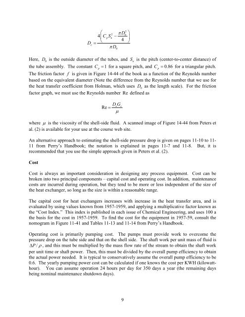
De⎛ π D4⎜CSp4=⎝π D22 0n−0⎞⎟⎠Here, D0is the outside diameter of the tubes, and Snis the pitch (center-to-center distance) ofthe tube assembly. The constant Cp= 1 for a square pitch, and Cp= 0.86 for a triangular pitch.The friction factor f is given in Figure 14-44 of the book as a function of the Reynolds numberbased on the equivalent diameter (Note the difference from the Reynolds number that we use forthe heat transfer coefficient from Holman, which uses D0as the length scale). For the frictionfactor graph, we must use the Reynolds number Re defined asDGµe sRe =where µ is the viscosity of the shell-side fluid. A scanned image of Figure 14-44 from Peters etal. (2) is available for your use at the course web site.An alternative approach to estimating the shell-side pressure drop is given on pages 11-10 to 11-11 from Perry’s Handbook; the notation is explained in pages 11-7 and 11-8. But, it isrecommended that you use the simple approach given in Peters et al. (2).CostCost is always an important consideration in designing any process equipment. Cost can bebroken into two principal components – capital cost and operating cost. In addition, maintenancecosts are incurred during operation, but they tend to be more or less independent of the size ofthe heat exchanger, so long as the size is within a reasonable range.The capital cost for heat exchangers increases with increase in the heat transfer area, and isevaluated by using values known from 1957-1959, and applying a multiplicative factor known asthe “Cost Index.” This index is published in each issue of Chemical Engineering, and uses 100 athe basis for the cost in 1957-1959. To find the cost for the equipment in 1957-59, consult thenomogram in Figure 11-41 and Tables 11-13 and 11-14 from Perry’s Handbook.Operating cost is primarily pumping cost. The pumps must provide work to overcome thepressure drop on the tube side and that on the shell side. The shaft work per unit mass of fluid is∆ P / ρ , and this must be multiplied by the mass flow rate of the stream to obtain the shaft workper unit time or shaft power. Then, this must be divided by the overall pump efficiency to obtainthe actual power needed. It is typical to conservatively assume the overall pump efficiency to be0.6. The yearly pumping power cost can be calculated if one knows the cost per KWH (kilowatthour).You can assume operation 24 hours per day for 350 days a year (the remaining daysbeing nominal maintenance shutdown days).9