Plant layout

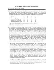
Some of the objectives of the plant layout1. Minimize investment in equipment2. Minimize overall production time3. Utilize existing space most effectively4. Minimize material handling cost3

Systematic Layout PlanningInput Data and ActivitiesFlow of materialsActivity RelationshipsRelationship DiagramSpace RequirementsSpace AvailabilitySpace Relationship DiagramModifying ConsiderationsPractical LimitationsDevelop Layout AlternativesEvaluation4

From – to chart• Provides information concerning thenumber of material handling trips betweendepartments (work centers)5

From-to Chart ExampleComponentProductionquantity / dayRouting1 30 ACBDE2 12 ABDE3 7 ACDBEComponent 1 and 2 have the same size. Component 3is almost twice as large. Therefore, moving two units ofcomponents 1 or 2 is equivalent to moving one unit ofcomponent 3. Show material flows between machineson a from-to chart.6

Machine Sequencing• Machining centers (departments) are laidout in such way that the total forward flowson the line is maximized, or total backwardflows are minimized.• Hollier developed two heuristic algorithmsthat can achieve ordering of machines forminimizing backtrack flows8

Hollier Method 1Step 1:Develop the “From-To” chart from part routing data.The data contained in the chart indicates numbers ofparts moves between machines (or work stations) inthe cell. Moves into and out of the cell are notincluded in the chart.Step 2:Determine the “From” and “To” sums foreach machine. This is accomplished by summing allof the “From” trips and “To” trips for each machine.9

Hollier Method 1Step 3:Assign machines to the cell based on minimum“From” or “To” sums. The machine having thesmallest sum is selected. If the minimum value isa “To” sum, then the machine is placed at thebeginning of the sequence. If the minimum valueis a “From” sum, then the machine is placed at theend of the sequence.10

Hollier Method 1Tie breaker rules: If a tie occurs between minimum “To” sums orminimum ”From” sums, then the machine with theminimum “From/To” ratio is selected. If both “To” and “From” sums are equal for aselected machine, it is passed over and themachine with the next lowest sum is selected. If a minimum “To” sum is equal to a minimum“From” sum, then both machines are selected andplaced at the beginning and end of the sequence,respectively.11

Hollier Method 1Step 4:Reformat the From-To chart. After each machinehas been selected, restructure the From-To chartby eliminating the row and column correspondingto the selected machine and recalculate the“From” and “To” sums.Step 5:Repeat steps 3 and 4 until all machines havebeen assigned.12

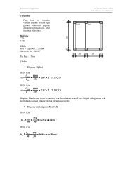
Example 5.1An analysis of 50 parts processed on four machines has beensummarized in the From-to chart of the following table.To: 1 2 3 4From: 1 0 5 0 252 30 0 0 153 10 40 0 04 10 0 0 0Additional information is that 50 parts enter the machinegrouping at machine 3, 20 parts leave after processing atmachine 1, 30 parts leave after machine 4. Determine alogical machine arrangement using Hollier method 1.13

Example 5.1 (solution)Iteration No.1To: 1 2 3 4 “From” SumsFrom: 1 0 5 0 25 302 30 0 0 15 453 10 40 0 0 504 10 0 0 0 10“To” Sums 50 45 0* 40 135* The minimum sum value is the “To” sum for machine 3.Machine sequence:314

Example 5.1 (solution)Iteration No.2To: 1 2 4 “From” SumsFrom: 1 0 5 25 302 30 0 15 454 10 0 0 10“To” Sums 40 5* 40 85* The minimum sum value is the “To” sum for machine 2.Machine sequence:3 215

Example 5.1 (solution)Iteration No.3To: 1 4 “From” SumsFrom: 1 0 25 254 10 0 10*“To” Sums 10* 25 35* There are two minimum sum values in this chart.The minimum “To” sum value for machine 1 is equal tothe minimum “From” sum value for machine 4.Machine sequence:3 2 1 416

Flow diagram101550 in4030253 2 1 430 out5 1020 out17

Percentage of in-sequence moves(%) which is computed by adding all of the values representingin-sequence moves and dividing by the total number of moves101550 in4030253 2 1 430 out5 1020 outNumber of in-sequence moves = 40 + 30 + 25 = 95Total number of moves = 95 + 15 + 10 + 10 + 5 = 135Percentage of in-sequence moves = 95/135 = 0.704 = 70.4%18

Percentage of backtracking moves(%) which is computed by adding all of the values representingbacktracking moves and dividing by the total number of moves101550 in4030253 2 1 430 out5 1020 outNumber of backtracking moves = 10 + 5 = 15Total number of moves = 95 + 15 + 10 + 10 + 5 = 135Percentage of backtracking moves = 15/135 = 0.704 = 11.1%19

Activity relationship analysis• A number of factors other than materialhandling cost might be of primary concernin layout design• Activity relationship chart (REL chart)should be constructed in order to realizethe closeness rating between departments20

An example of REL chartA =Absolutely necessaryE =Especially importantI =ImportantO =Ordinary closenessU =UnimportantX =Undesirable21

Proportion of each ratingRatingA & XProportion tothe whole relations 5%E 10%I 15%O 20%Hence,U 50%22

Relationship diagram• Constitutes the 3rd step of SLP. Itconverts the information in the REL chartinto a diagram• REL diagram can either be constructedmanually or by using computer algorithms23

Layout algorithms• In general, layout algorithms are of two types asImprovement and Construction• Improvement algorithms begin with an initiallayout and search for improved solutions CRAFT (require quantitative flow input) COFAD• Construction algorithms add departments to thelayout, one by one, until all departments havebeen palced ALDEP CORELAP (require qualitative input) PLANET RDP (Relationship Diagramming Process)24

Relationship Diagramming Process (RDP)RDP is a construction algorithm, which addsdepartments to the layout one by one until alldepartments have been placed.Stage 1: Involves 5 steps to determine the order ofplacementStep 1 the numerical values are assigned tothe closeness rating as:A= 10 000, E= 1000, I= 100, O= 10, U= 0, X= – 10 00025

Relationship Diagramming Process (RDP)Step 2 TCR (Total Closeness Rating) for eachdepartment is computed. TCR refers to the sum ofthe absolute values for the relationships with aparticular department.Step 3 The department with the greatest TCRis selected as the first placed department in thesequence of placement.26

Relationship Diagramming Process (RDP)Step 4 Next department in the sequence ofplacement is determined to satisfy the highestcloseness rating with the placed department(s).With respect to the closeness priorities A>E>I>O>UStep 5 Departments having X relationship withthe placed department(s) are labeled as the lastplaced department.Note: If ties exist during this process, TCR valuesare utilized to break the ties arbitrarily.27

Relationship Diagramming Process (RDP)Stage 2: Involves 3 steps to determine the relativelocations of the departmentsStep 6 Calculate Weighted Placement Value(WPV) of locations to which the next department inthe order will be assigned. WPV refers to the sum ofthe numerical values for all pairs of adjacentdepartment(s). When a location is fully adjacent, itsweight equals to 1.0, and when it is partially adjacentits weight equals to 0.5.28

Relationship Diagramming Process (RDP)Step 7 Evaluate all possible locations in counterclock-wise order, starting at the western edge of thepartial layout.Step 8 Assign the next department to the locationwith the largest WPV.Note: If ties exist during this process, first locationwith the largest WPV is selected.29

Example 5.2Given the activity relationship diagram (REL)determine the layout of departments using RDP.30

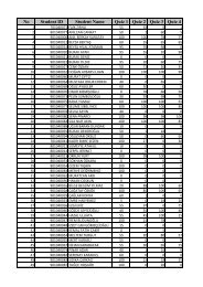
Example 5.2 (solution) 1 st stageCalculate the Total closeness ratings (TCR) withvalues of A=10,000; E=1000; I=100; O=10; U=0Department A E I O U X TCR1 Offices 0 1 0 1 3 0 10102 Foreman 0 1 3 1 0 0 13103 Conf. room 0 1 1 0 3 0 11004 Receiving 1 0 1 0 3 0 101005 Parts ship. 1 1 0 0 3 0 110006 Storage 2 0 1 0 2 0 20100Selected as the firstplaced department31

Example 5.2 (solution) 1 st stageNext department in the sequence of placement is determined tosatisfy the highest closeness rating with the placed department(s).With respect to the closeness priorities A>E>I>O>UPlaced Dept.654 or 5 will be selectedas the next to be placedIf ties exist during this process, TCR values are utilized to break theties arbitrarily. TCR 5 = 11,000 > TCR 4 = 10,1005 is selected as the next to be placed32

Example 5.2 (solution) 1 st stageWith respect to the closeness priorities A>E>I>O>UPlaced Dept.6544 is selected as the next to be placed33

Example 5.2 (solution) 1 st stageWith respect to the closeness priorities A>E>I>O>UPlaced Dept.65422 is selected as the next to be placed34

Example 5.2 (solution) 1 st stageWith respect to the closeness priorities A>E>I>O>UPlaced Dept.6542313 is selected as the next to be placedPlacement sequence: 6,5,4,2,3,135

Example 5.2 (solution) 2 nd stageFullyadjacentWPV1 = 1(10,000)= 10,0008 7 6Next to1652 3 4WPV2 = 0.5(10,000) = 5000Partiallyadjacentbe placedWPV3 = 1(10,000) = 10,000WPV4 = 0.5(10,000) = 5000WPV5 = 1(10,000) = 10,000WPV6 = 0.5(10,000) = 5000WPV7 = 1(10,000) = 10,000WPV8 = 0.5(10,000) = 5000Placing Order654231A = 10,00036

Example 5.2 (solution) 2 nd stage10129 8 75 6 63 4 5Next tobe placedWPV1 = 1(0) = 0WPV2 = 0.5(0) = 0WPV3 = 1(0)+0.5(10,000) = 5000WPV4 = 0.5(0)+1(10,000) = 10,000WPV5 = 0.5(10,000) = 5000WPV6 = 1(10,000) = 10,000WPV7 = 0.5(10,000) = 5000WPV8 = 1(10,000)+0.5(0) = 10,000WPV9 = 0.5(10,000)+1(0) = 5000WPV10 = 0.5(0) = 0PlacingOrder4231A = 10,000 ; U = 037

Example 5.2 (solution) 2 nd stage121211 10 95 6 83 4 74 5 6WPV1 = 1000WPV2 = 500WPV3 = 1150WPV4 = 50WPV5 = 100WPV6 = 50WPV7 = 150WPV8 = 150WPV9 = 50WPV10 = 600WPV11 = 1050WPV12 = 500Next tobe placedPlacingOrder231E = 1000 ; I = 10038

Example 5.2 (solution) 2 nd stage1212311 10 95 6 82 4 74 5 6WPV1 = 50WPV2 = 100WPV3 = 50WPV4 = 100WPV5 = 50WPV6..12 = 0Next tobe placedPlacingOrder31I = 100 ; U = 039

Example 5.2 (solution) 2 nd stage141212133311 10 95 6 82 4 74 5 6WPV1 = 1000WPV2 = 500WPV3 = 1005WPV4 = 510WPV5 = 5WPV6..12 = 0WPV13 = 1005WPV14 = 500Next tobe placedPlacingOrder1E = 1000 ; O = 10 ; U = 040

Example 5.2 (solution) 2 nd stageFinal relationship daigram of the layout31562 441

CRAFT-(Computerized RelativeAllocation of Facilities Technique)• First computer-aided layout algorithm (1963)• The input data is represented in the form of aFrom-To chart, or qualitative data.• The main objective behind CRAFT is to minimizetotal transportation cost:• Improvement-type layout algorithmf ij = material flow between departments i and jc ij = unit cost to move materials betweendepartments i and jd ij = rectilinear distance between departmentsi and j42

Steps in CRAFT• Calculate centroid of each department and rectilineardistance between pairs of departments centroids (storedin a distance matrix).• Find the cost of the initial layout by multiplying the From-To (flow) chart, Unit cost matrix, and From-To (distance) matrix• Improve the layout by performing all-possible two orthree-way exchanges At each iteration, CRAFT selects the interchange that results inthe maximum reduction in transportation costs These interchanges are continued until no further reduction ispossible43

Example (Craft)Initial layoutTotal movement cost = (20 x 15) + (20 x 10) + (40 x 50)+ (20 x 20) + (20 x 5) + (20 x 10) = 320044

SolutionThe possible interchanges for the initial layout are:45

AB interchangingMovement Cost = (20 x 15) + (30 x 10) + (10 x 50)+ (10 x 20) + (30 x 5) + (20 x 10) = 1650The reduction in movement cost = 3200 – 1650 = 155046

AC interchanginggx C = [(100)15+(200)5]/300 = 8.33gy C = [(100)5+(200)10]/300 = 8.33Movement Cost = (10 x 15) + (20 x 10) + (10 x 50)+ (23.34 x 20) + (20 x 5) + (30 x 10) = 1716.8The reduction in movement cost = 3200 – 1716.8 = 1483.247

Other interchanges and savingsADSavings: 0 BC Savings: 0BDSavings: 1383.2 CD Savings: 155048

Current layout after AB interchangeWith this layout new pair wise interchanges are attempted as follows:A D, B C, C DA B not considered since it will result no savingsA C not considered since they don’t have common bordersB D not considered since they don’t have common borders49

Interchanges and savingsADBCSavings: 0 Savings: 0CD Savings: 0So, the current layout is the bestlayout that CRAFT can find50