Webless Migratory Game Bird Program - U.S. Fish and Wildlife Service

U.S. Fish & Wildlife Service
Webless Migratory Game Bird Program
Project Abstracts – 2010-11

Webless Migratory Game Bird
Program
Project Abstracts – 2010 and 2011
Compiled by Tom Cooper
Project Officer
U.S. Fish and Wildlife Service
Division of Migratory Bird Management
5600 American Blvd. West, Suite 950
Bloomington, MN 55437
July 2012
Suggested citation:
Cooper, T. R. (Compiler). 2012. Webless Migratory Game Bird Program, Project Abstracts – 2010 and
2011. United States Department of the Interior, Fish and Wildlife Service, Bloomingtion, MN USA.
140p.
The purpose of this report is to provide updated information on projects being funded through the U.S.
Fish and Wildlife Service’s Webless Migratory Game Bird Program. Any specific questions on projects
should be addressed directly to the abstract authors.
Cover photo by Todd Sanders, U.S. Fish and Wildlife Service, band-tailed pigeons visiting a mineral
site station.

CONTENTS
Development and History of the Webless Program
History and Administration of the Webless Migratory Game Bird Program, 1995-2012 1
David D. Dolton and Thomas R. Cooper
Webless Migratory Game Bird Program Project Abstracts
Mourning Doves
Harvest and Crippling Rates of Mourning Doves in Missouri 6
John H. Schulz, Thomas W. Bonnot, Joshua J. Millspaugh, and Tony W. Mong
Development of a Temporally and Spatially Explicit Model of Mourning Dove Recruitment for Harvest Mgmt. 8
David W. Miller
Improving the Design and Count Methodology of the Mourning Dove Call-count Survey in the Eastern and Central
Management Units: Pilot Study 12
Frank F. Rivera-Milàn, Mark Seamans, and Rebecca Rau
White-winged Doves
Development and Evaluation of a Parts Collection Survey for White-winge Doves in the Southeastern United States 16
Bret A. Collier, Brian L. Pierce, Corey Mason, Kyle Hand, and Taylor Jacobs
Band-tailed Pigeons
Band-tailed Pigeon Use of Supplemental Sodium and Calcium 21
Todd A. Sanders
Sandhill Cranes
Population Genetic Structure in the Eastern Population of Greater Sandhill Cranes 33
Mark E. Berres, Jeb A. Barzen, and Matthew A. Hayes
An Initial Evaluation of the Annual Mid-Continent Sandhill Crane Population Survey 38
Aaron T. Pearse, Gary L. Krapu, and David A. Brandt
Sandhill Crane Nest and Chick Survival in Nevada 42
Chad W. August, James S. Sedinger, and Christopher A. Nicolai
The Use of Satellite Telemetry to Evaluate Migration Chronology and Breeding, Migratory, and Wintering
Distribution of Eastern Population Sandhill Cranes 52
Dave Fronczak and David E. Andersen
American Woodcock
Habitat Use and Origins of American Woodcock Wintering in East Texas 59
Dan S. Sullins, Warren C. Conway, Christopher E. Comer, and David A. Haukos

Assessment of Techniques for Evaluating American Woodcock Population Response to Best Management Practices
Applied at the Demonstration-area Scale 67
Kyle O. Daly, David E. Andersen, and Wayne L. Brininger Jr.
Factors Affecting Detection of American Woodcock on Singing-Ground Surveys 75
Stefanie M. Bergh and David E. Andersen
Marshbirds
The Effect of Waterfowl Impoundments on Sora and Virginia Rail Populations 85
Brian J. Olsen and Ellen P. Robertson
Nesting, Brood Rearing, and Winter Habitat Selection of King Rails and Clapper Rails within the ACE Basin, South
Carolina 92
William E. Mills, Ernie P. Wiggers, Catherine E. Ricketts, Jeffrey Hepinstall-Cymerman, and Sara H.
Schweitzer
Evaluation of an Expert-based Landscape Suitability Model for King Rails in the Upper Mississippi River and Great
Lakes Joint Venture Region 97
David G. Krementz and Jason R. Bolenbaugh
Implementation of the National Marshbird Monitoring Program in Ohio 99
David E. Sherman and John W. Simpson
Implementation of a National Marshbird Monitoring Program: Using Wisconsin as a Test of Program Study Design 103
Andy Paulios and Ryan Brady
Estimating Population Trends, Relative Abundance, and Effects of Management Actions on 7 Species of Webless
Migratory Game Birds 109
Courtney J. Conway, Leonard Santisteban, and Christopher P. Nadeau
Expanding the Michigan Marsh Bird Survey to Facilitate Conservation at Multiple Scales 112
Michael J. Monfils and David L. Cuthrell
Development of a Winter Survey for Wilson’s Snipe in the Mississippi Flyway 116
David G. Krementz and J. Matthew Carroll
Developing Optimal Survey Techniques for Monitoring Population Status of Rails, Coots, and Gallinules 123
Courtney J. Conway, Mark Woodrey, Christopher Nadeau, and Meaghan Conway
King Rail Nesting and Brood Rearing Ecology in Managed Wetlands 126
David G. Krementz and Karen L. Willard
Appendices
Appendix I. Projects Funded by the FY2012 Webless Migratory Game Bird Program 134
Appendix II. Summary of FWS Region 5 Projects Supported by the Webless Migratory Game Bird Program 136

HISTORY AND ADMINISTRATION OF THE WEBLESS MIGRATORY GAME BIRD
PROGRAM, 1995-2012
THOMAS R. COOPER, U.S. Fish and Wildlife Service, Division of Migratory Bird Management, 5600
American Blvd. West, Suite 950, Bloomington, MN 55437, USA (tom_cooper@fws.gov)
DAVID D. DOLTON (retired), U.S. Fish and Wildlife Service, Office of Migratory Bird Management, PO Box
25486 DFC, Denver, CO 80225-0486, USA
Introduction
The Webless Migratory Game Bird (WMGB) Program
is an outgrowth of the WMGB Research Program
(1994-present) and the WMGB Management Program
(2007-present). The revised WMGB Program was
designed to provide cooperative funding for both
research and management activities from the U.S. Fish
and Wildlife Service (USFWS), state wildlife
agencies, and other sources for projects benefitting the
16 species of migratory game birds in North America
(Table 1).
Table 1. The 16 species of migratory shore and upland
game birds eligible for funding through the Webless
Migratory Game Bird Program.
Common Name Scientific Name
King Rail Rallus elegans
Clapper Rail Rallus longirostris
Virginia Rail Rallus limicola
Sora Porzana carolina
Purple Gallinule Porphyrio martinica
Common Gallinule 1 Gallinula galeata
American Coot Fulica americana
Sandhill Crane Grus canadensis
Wilson’s Snipe Gallinago delicata
American Woodcock Scolopax minor
Band-tailed Pigeon Patagioenas fasciata
Scaly-naped Pigeon Patagioenas squamosa
Zenaida Dove Zenaida aurita
Mourning Dove Zenaida macroura
White-winged Dove Zenaida asiatica
White-tipped Dove Leptotila verreauxi
1 Formerly Common Moorhen (Gallinula chloropus)
History
The WMGB Program is an outgrowth of several
funding initiatives, both past and present. The first
effort was the Accelerated Research Program (1967-
1982). Congressional funding of the ARP was
$250,000 annually. Of this total, $175,000 was
1
contracted to states: $50,000 was used directly by the
USFWS to support 2 field stations to study woodcock
and doves; and, $25,000 was retained by the USFWS
to administer the program. The ARP ended when
funding for the program was eliminated due to
USFWS budget constraints in 1982. In 1984, the
International Association of Fish and Wildlife
Agencies (now AFWA) formed the Migratory Shore
and Upland Game Bird (MSUGB) Subcommittee.
One goal of the subcommittee was to reinstate a
webless game bird research program. To accomplish
this goal, the subcommittee documented the past
accomplishments of the ARP and lobbied for
reinstatement of a webless research program. The
efforts and persistence of the MSUGB Subcommittee
came to fruition in the fall of 1994 when funding
became available. The new program was titled the
WMGB Research Program. Projects were selected for
funding beginning in 1995 with funding being
obligated for the entire project. Detailed information
about the history of the ARP and WMGB Research
Programs can be found in Dolton (2009).
The WMGB Research Program was funded at various
levels during 1995-2006; however, funding was
suspended due to budget limitations in 2003 and 2004.
Funding was reinstated in 2005 at a level of
$250,000/year, with $30,000 of the total being
obligated for webless projects in USFWS Region 5
(Northeast U.S.). In 2007, the USFWS received
additional funding for MSUGB work ($487,000/year).
The primary purpose of the new funding was to
address the management needs of MSUGB. From
2007-2009, funding was directed towards supporting
mourning dove banding in several states and other
management related projects for woodcock, rails, and
sandhill cranes.
Another key contribution made by the MSUGB
Committee was the publication of the book entitled
Migratory Shore and Upland Game Bird Management
in North America (Tacha and Braun 1994). This was a

evised and updated version of the book edited by
Sanderson (1977). Priority research and management
activities identified in these books served as a tool for
evaluating proposals submitted to the WMGB
Research Program for funding.
AFWA’s MSUGB Working Group (formerly MSUGB
Subcommittee) provided key support in acquiring the
additional funding. Due to the addition of funding for
management-related projects (as opposed to research
only projects), cooperators made the decision to drop
“research” from the title of the WMGB Program.
The MSUGB Working Group created the MSUGB
Task Force in 2006 in order to update the priority
research and management needs identified in Tacha
and Braun (1994) and to develop funding strategies for
the identified priorities. The task force decided that
the best method to identify priorities and estimate
costs for completing the priorities was to convene a
series of workshops for the webless species identified
in Table 1. The workshops were designed to include
broad representation from experts (e.g., federal and
state agencies, conservation organizations, and
university researchers) for each species-specific group.
To date, the MSUGB Task Force has completed
strategies identifying priority information needs for:
(1) mourning and white-winged doves, (2) hunted rails
and snipe, (3) sandhill cranes, (4) American
woodcock, and (5) American coots, purple gallinules,
and common moorhens. The final workshop covering
the remaining species (Zenaida doves, white-tipped
doves, scaly-naped pigeons, and band-tailed pigeons)
was completed in early 2011. The completed priority
information-need strategies are available on-line at:
www.fws.gov/migratorybirds/NewReportsPublications/Rese
arch/WMGBMR/WMGBMR.html.
These webless funding programs have proved to be
invaluable in providing much-needed funding for
webless species that receive considerably less attention
than waterfowl. To date, the Webless Program has
supported a total of 118 research and management
related projects totaling $5.5 million in WMGB
Research and Management Program funds. The
WMGB Program funds have generated matching
contributions of $10 million from cooperators for a
total $15.5 million being expended on webless species
(Table 2). Projects completed through the program
have resulted in improved knowledge and
management of webless migratory game birds.
Previous annual abstract reports containing results of
projects completed through the program are available
on-line at:
www.fws.gov/migratorybirds/NewReportsPublications
/Research/WMGBMR/WMGBMR.html
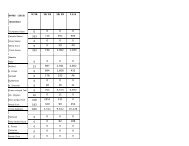
Table 2. Summary of projects funded through the Webless Migratory Game Bird Program, 1995-2012 1 .
No. of
WMGBP
Matching Total Project
Species Group
projects
Funds
Funds
Cost
Doves and Pigeons 41 $2,166,278 $3,953,396 $6,119,674
American Woodcock 16 $1,137,748 $2,161,318 $3,299,066
Sandhill Crane 20 $887,329 $2,035,237 $2,922,566
Marshbirds 2 25 $1,115,356 $1,845,290 $2,960,646
Webless Workshops/other 3 16 $168,095 $41,213 $209,308
Total 118 $5,474,806 $10,036,454 $15,511,260
1 Includes projects funded through FY 2012 Webless funds
2 Includes sora, Virginia rail, king rail, clapper rail, purple gallinule, common gallinule, American coot, and Wilson’s snipe
3 Includes a series of 6 workshops held during 2008-10 where priority information needs for webless species were identified
2

Program Administration
The USFWS Project Officer for the WMGB Program
distributes an annual request for proposals (RFP) in
May to USFWS Flyway Representatives, Regional
Migratory Bird Coordinators, USGS-Biological
Research Division (BRD) Regional Offices, and the
USGS Cooperative Research Units office. In addition,
the funding opportunity is posted at: www.grants.gov.
Flyway Representatives are responsible for
distributing the RFP to biologists in their respective
states. State biologists, in turn, are asked to send the
information to other state personnel, universities, and
any others who may be interested. Migratory Bird
Coordinators forward the letter to National Wildlife
Refuges and other federal offices. USGS-BRD
Regional Offices are asked to forward the RFP to all
their respective Science and Technology Centers,
while the Cooperative Research Units office
distributes the RFP to all Cooperative Fish and
Wildlife Research Units. Funding proposals may be
submitted for any webless migratory game bird
identified in Table 1. Proposals may be orientated
toward research or management-related projects. At
least 1/3 of the total project cost must come from a
funding source other than the WMGB Program. Inkind
services, such as salaries of state employees and
vehicle expenses, are acceptable as matching funds.
Additionally, a letter of support is required for each
proposal from the state in which it originates.
Proposals for the program are due by November 1
each year.
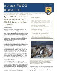
Four regional review committees (Fig. 1) that follow
the boundaries of the North American Flyways (Fig. 2)
rank all proposals submitted to the program. The
Flyway-based committees are composed of individuals
with knowledge of the research and management
needs for these species. The chairperson of each
Flyway-based review committee serves on a National
Review Committee (NRC), which makes final project
selections based on input from each Flyway-based
committee. The NRC is composed of the Flywaybased
Chairs, the U.S. Fish and Wildlife Service
Program Manager, and Representatives from the
Migratory Shore and Upland Game Bird Support Task
Force. The NRC evaluates and ranks proposals based
on how well the proposals address the priority
information needs that have been identified for the 16
species of Migratory Shore and Upland Game Birds
(see Appendix A for specific priorities). After project
selection, the NRC is responsible for developing an
explanation documenting why successful projects were
3
selected for funding. In addition, the NRC provides
unsuccessful applicants with comments on why their
project was not funded.
Pacific Flyway
Review Comm.
RFP Developed and Released
Proposals Developed by PIs
Central Flyway
Review Comm.
Mississippi Flyway
Review Comm.
National Review Comm.
Summary Report w/ decision rationales
Priority Projects funded
Atlantic Flyway
Review Comm.
Figure 1. Diagram of review process for proposals
submitted to the Webless Migratory Game Bird Program.
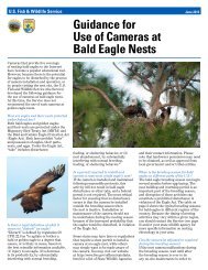
Figure 2. Map of North American Flyway boundaries in
the United States. Proposals working with the 16 species
identified in Table 1 will be accepted from throughout North
America.

Literature Cited
Dolton, D.D. (compiler). 2009. History and
administration of the Webless Migratory Game
Bird Research Program, 1995-2008. In Webless
Migratory Game Bird Research Program, Project
Abstracts – 2008. United States Department of the
Interior, Fish and Wildlife Service, Denver,
Colorado. 66 pp.
www.fws.gov/migratorybirds/NewReportsPublicat
ions/Research/WMGBMR/WMGBR%20ABSTR
ACTS%202008%20rev.pdf
Sanderson, G.C., editor. 1977. Management of
migratory shore and upland game birds in North
America. International Association of Fish and
Wildlife Agencies, Washington, D.C. 358 pp.
Tacha, T.C., and C.E. Braun, editors. 1994.
Migratory shore and upland game bird
management in North America. International
Association of Fish and Wildlife Agencies.
Washington, D.C. 223 pp
4

Appendix A – Priority Information Needs for Migratory Shore and Upland Game Birds
Priority information needs have been developed for the following groups: 1) mourning and white-winged doves; 2) hunted
rails (sora, clapper, king, and Virginia) and Wilson’s snipe; 3) sandhill cranes; 4) American woodcock; 5) American coots,
common moorhens, and purple gallinules; and 6) band-tailed pigeon, scaly-naped pigeon, Zenaida dove, and white-tipped
dove. Proposals should address the priorities listed below for each species group. A full description and justification are
available at www.fws.gov/migratorybirds/NewReportsPublications/Research/WMGBMR/WMGBMR.html.
Mourning and White-winged Dove Priorities:
� Implement a national banding program for doves
� Implement a national dove parts collection survey
� Develop independent measures of abundance and/or trends for doves
� Create a database of predictors of dove vital rates
Hunted Rails and Wilson’s snipe Priorities:
� Implement a national monitoring program
� Continue to improve the Harvest Information Program sampling frame
� Improve the rails and snipe parts collection survey
� Estimate vital rates to support population modeling
Sandhill Crane Priorities:
� Improve Sandhill Crane Harvest-Management Decision Structures
� Improve the Eastern Population Sandhill Crane Survey
� Better understand distribution and population trends for sandhill crane populations in the west
� Assess Effects of Habitat Changes on the Rocky Mountain Population of Sandhill Cranes
� Improve Population Abundance Estimates for the Mid-Continent Population of Sandhill Cranes
American Woodcock Priorities:
� Develop a demographic-based model for assessing American woodcock population response to harvest and habitat
management
� Develop communication strategies to increase support for policies and practices that benefit American woodcock
and other wildlife of young forests
� Improve understanding of migration, breeding, and wintering habitat quality for American woodcock
� Improve the American woodcock Singing-ground Survey
American Coot, Common Moorhen, and Purple Gallinule Priorities:
� Implement a national marshbird monitoring program
� Support National Wetlands Inventory updates and improvements
� Continue to improve the Harvest Information Program sampling frame
� Determine the origin of harvest in select high harvest states in order to help inform monitoring programs
Band-tailed Pigeon, Zenaida Dove, White-tipped Dove, and Scaly-naped Pigeon Priorities:
� Reliable demographics of band-tailed pigeons
� Association of food availability with abundance and distribution of band-tailed pigeons
� Status assessment of white-tipped doves in south Texas to determine distribution, population abundance, and
biology
� Population and harvest data collected annually for Zenaida doves and scaly-naped pigeons
� Adaptive harvest strategy for Zenaida doves and scaly-naped pigeons
5

Webless Migratory Game Bird Research Program Projects
Progress to Date
Mourning Doves
HARVEST AND CRIPPLING RATES OF MOURNING DOVES IN MISSOURI
JOHN H. SCHULZ, 1 Missouri Department of Conservation, Resource Science Center, 1110 South College
Avenue, Columbia, MO 65201, USA (John.H.Schulz@mdc.mo.gov)
THOMAS W. BONNOT, Department of Fisheries and Wildlife Sciences, University of Missouri, 302 Anheuser-
Busch Natural Resources Building, Columbia, MO 65211, USA
JOSHUA J. MILLSPAUGH, Department of Fisheries and Wildlife Sciences, University of Missouri, 302
Anheuser-Busch Natural Resources Building, Columbia, MO 65211, USA
TONY W. MONG, 2 Department of Fisheries and Wildlife Sciences, University of Missouri, 302 Anheuser-
Busch Natural Resources Building, Columbia, MO 65211, USA
Final Report
Mourning dove (Zenaida macroura) harvest
management requires an assessment of birds shot and
not recovered (hereafter crippled doves) to determine
harvest mortality. However, estimating crippling rates
is challenging. We estimated mourning dove harvest
mortality in Missouri, which included crippling rates,
by monitoring radio-marked doves. We also
compared crippling rates of radio-marked doves to
hunter-reported estimates of crippling. During 2005–
2008, we estimated annual harvest mortality between
23–30% on one locally managed public hunting area.
Crippling rates ranged from 18–50% of harvest
mortality in radio-marked doves (Table 1). In
comparison, hunter-reported crippling rates during
2005–2011 (14−18%) were, on average, 30% lower
but more consistent than estimates from radio-marked
doves (Table 1). During 2005–2008, harvest mortality
of radio-marked doves was 27%, with one quarter of
this mortality coming from crippled doves (Table 1).
These results demonstrate crippling was a sizeable
component of dove harvest; however, it was within the
range of earlier crippling rate estimates for doves.
Bias in hunter-reported crippling rates could result in
overharvest if not accounted for. Future harvest
management decisions should not overlook the
potential impacts of crippling on populations,
especially on locally managed public hunting areas.
Field work on this project concluded during 2008 with
analysis and reporting on various other manuscripts;
6
this abstract is one of several documents constituting
the final report. Funding and support for this work
were provided by the Missouri Department of
Conservation–Resource Science Division, the
University of Missouri–Department of Fisheries and
Wildlife Sciences, and by the U.S. Fish and Wildlife
Service Webless Game Bird Research Grant Program.
David Dolton (retired USFWS) watches Tony Mong
implant a subcutaneous radio transmitter in a mourning
dove captured and released on the James A. Reed
Memorial Wildlife Area. Photo by Missouri DOC

Table 1. Harvest and crippling of mourning doves on the James A. Reed Memorial Wildlife Area during 2005–2011.
Harvest rates (h) and crippling rates (c) of were derived from numbers of radio-marked recovered and crippled doves
available on the area during the first 2-days of the annual managed hunt. Estimated hunter-reported crippling rates ( ) are
based on surveys of all hunters visiting the area during the same 2-day period.
Radio-marked data Hunter-reported data
Year Available a Recovered b Crippled c
Harvest
mortality d h e c f
Recovered Crippled
2005 73 14 3 17 0.23 0.18 6039 1076 0.15
2006 88 20 6 26 0.3 0.23 5000 1006 0.17
2007 21 3 3 6 0.29 0.5 1818 408 0.18
2008 41 8 3 11 0.27 0.27 2406 479 0.17
2009 -- d -- -- -- -- -- 2052 415 0.17
2010 -- -- -- -- -- -- 1745 363 0.17
2011 -- -- -- -- -- -- 2088 330 0.14
Total 223 45 15 60 0.27 0.25 21148 4077 0.16
a Sample size of radio-marked doves detected on the area during harvest.
b Radio-marked doves that were recovered: number of radio-marked doves shot,
recovered by hunters, and checked by hunters.
c Radio-marked doves that were crippled: number of radio-marked doves shot but not
recovered by hunters.
d Harvest mortality of radio-marked doves: recovered radio-marked doves + crippled
radio-marked doves.
e Harvest rate of radio-marked doves: proportion of radio-marked doves that were
available on the site that were either shot and recovered by hunter (recovered radiomarked
dove) or shot but not recovered by hunter (crippled radio-marked dove).
f Crippling rate of radio-marked doves: proportion of harvest mortality of radio-marked
doves that were crippled (shot but not recovered by hunter).
7

DEVELOPMENT OF A TEMPORALLY AND SPATIALLY EXPLICIT MODEL OF
MOURNING DOVE RECRUITMENT FOR HARVEST MANAGEMENT
DAVID A.W. MILLER, U.S. Geological Survey, Patuxent Wildlife Research Center, 12100 Beech Forest Road,
Laurel, MD 20708. (davidmiller@usgs.gov)
Progress Report; Expected Completion: Fall 2013
Introduction
A coordinated effort by state and federal agencies
has been undertaken to improve our understanding
of the harvest dynamics of mourning doves and to
better manage populations. The mourning dove
national strategic harvest management plan was
developed as part of this effort, calling for the
implementation of an informed strategy for harvest
derived from predictions based on population
models of the species (USFWS 2004). Establishing
monitoring programs for population vital rates was a
critical component of the plan. This included
instituting a large-scale operational program for
monitoring reproductive rates and determining how
to integrate data from the monitoring program into
harvest decision making. In 2005, with the
cooperation of 22 state agencies, US Fish and
Wildlife Service personnel, and funding from the
Webless Migratory Gamebird Research Grant
program, a pilot harvest parts collection program
began as the first step in developing a national
program for monitoring dove recruitment rates
(Miller 2009, Miller and Otis 2010). This was
followed in 2007 with the implementation of a
national mail survey conducted by the US Fish and
Wildlife Service and which now serves as the
operational program for monitoring dove
recruitment. These wings are aged by state and
federal biologists at an annual wing bee that has
been hosted each year by the Missouri Department
of Conservation
This abstract summarizes results of the first year of a
new 3-year study funded by the Webless Migratory
Game Bird Research Program (U.S. Fish and
Wildlife Service). The work focuses on developing
an initial model for recruitment, which will serve as
a link between the recently implemented recruitment
monitoring effort and the development of a
population model that can be used in a decision
support framework for harvest management.
Previous work has suggested potentially useful
structure for a recruitment model that can be used in
the context of harvest decision making (Runge et al.
2002, USFWS 2004, AFWA 2008,Miller 2009, Otis
2010). Three basic components for such a model are:
1) Mean recruitment estimates: Previous work
has demonstrated large geographic variation
in dove recruitment rates (Miller and Otis
2010). Differences in recruitment among the
3 dove management units are a necessary
minimum that must be estimated when
determining harvest effects. Further work to
determine within region differences in
recruitment will provide further insights
about how life-history variation is structured
across the range of the mourning dove.
2) Environmental effects on annual variation:
Large-scale drivers of annual variation in
recruitment are likely to be due to annual
variation in weather (Runge et al. 2002,
AFWA 2008, Miller 2009). Weather
patterns can be correlated across large
spatial scales necessary to create
synchronized annual variation across regions
used for management. The degree to which
this will be useful part of a recruitment
model will depend on whether or not
correlated large-scale variation in
recruitment occurs, whether weather
predicts this recruitment variation, and
whether this variation can be incorporated
into predictions on a time-scale useful for
harvest decision making (AFWA 2008).
3) Density-dependent effects: Densitydependence
can have significant impacts on
recruitment rates (Runge et al. 2002) and has
important implications for harvest decision
making (Runge et al. 2006). Densitydependence
is one of the mechanisms that
can lead to surplus availability of birds for
harvest and therefore should be incorporated
into a useful model if it occurs for doves.
Though these factors are not exhaustive,
understanding them is an important first step in
predicting recruitment dynamics and serve as a
8

idge between current monitoring efforts and the
proposed harvest decision making framework.
Wings are scored annually at the Mourning Dove
Wing Bee held outside of Kansas City, Missouri.
Photo by David Miller
Completed Work
The first step in completing the project was to
develop a comprehensive analysis framework for
estimating recruitment parameters from the mail
survey data. The mourning dove parts survey has the
advantage of most wings collected during the first
weeks of September are local birds. Greater than
93% of band-returns for harvested doves come from
less than 100 km from where banding occurred.
Thus, the survey provides local replication across
their range that can be used to determine patterns.
Proper analysis that takes advantage of this
replication needs should account for the fact that
only a small number of wings are collected at any
location and that spatial autocorrelation is likely to
occur among collection points.
I have developed a hierarchical modeling framework
to analyze the data that addresses these issues. When
wings are collected the county where they were
harvested is recorded. Wings are assigned a spatial
location by the centroid of the county and are
aggregated to cells from hexagonal grid that spans
their range. The hierarchical model accounts for
sampling error related to sample size and local
variation within cells by treating the number of
hatch-year individuals in the sample as repeated
binomial samples. Spatial correlation among cells is
accounted for using a conditional autoregressive
(CAR) parameter. Accounting for spatial correlation
has the advantage of borrowing information among
cells when estimating recruitment. In addition,
accounting for spatial correlation is important to
address the lack of independence among close by
collection points for future work that will examine
factors related to recruitment variation.
As an initial proof of concept I conducted 2
analyses, the results of which were shared with state
cooperators at the Central Management Unit
Technical Meeting in March of this year. First I
estimated mean recruitment rates for each of the
cells using all years of data (Fig.1 – panel 1). The
results indicated a high-level of spatial correlation
among cells and are consistent with previous
analyses of the initial wing collection data (Miller
and Otis 2010). In general, recruitment was highest
in the eastern states and lower in the western states.
In the west, recruitment was higher in the northwest
and was lowest in a region that spanned from
Arizona to west Texas. The results indicate that very
different recruitment patterns occur among the 3
dove management units. This has implications when
estimating the impact of harvest on dove population
dynamics.
The second analysis I conducted was to estimate
annual variation in recruitment. In Fig. 1 (panel 2 –
6), I present annual differences from then mean
value in recruitment. Thus, positive values (yellow
and orange) indicate an above average year and
negative values (green) a below average year.
Although much noisier than the pattern for mean
recruitment, the results indicate that annual variation
in reproductive output may also be synchronized
across large areas. For example, in the eastern states
recruitment was nearly universally high in 2007 and
2011 and low in 2009 and 2010, with a split between
northern and southern states in the east during 2008.
Although preliminary, these results suggest that
relevant variation (i.e., differences at the
management level) occurs in annual recruitment
Next Steps
I am currently working on building more
comprehensive models for spatial variation. The
goal will be to determine how some simple habitat
measures (e.g., mean annual rainfall, forest cover,
and human development) relate to geographic
variation in recruitment. I anticipate finishing this
9

component of the project by this coming fall.
In addition, I have conducted preliminary analyses to
look at the relationship between weather and annual
recruitment. These indicate a strong role for summer
conditions in predicting reproductive output (Fig. 2).
However, these were based on a relatively short
sampling period (3 years) and ignored spatial issues.
Once wing data and weather covariates are available
for 2012, I will begin to integrate this component
into the estimated recruitment model.
Figure 2. Preliminary results suggest summer conditions
can affect mourning dove recruitment at the regional
level. This figure shows the relationship between
residuals for the annual proportion of hatch year wings in
the mail survey sample and the residual for the annual dry
heat index for 2007 to 2009. Each point represents values
for a single year and region combination (regions were
southeast, south-central, southwest, northeast, northcentral,
and northwest). Future work to explore these
patterns will incorporate additional years of data and a
more robust methodology to estimate effects
Acknowledgements
Special thanks goes to the efforts of all the state
agencies involved in the initial pilot recruitment
monitoring effort and the current monitoring effort.
Dave Otis, John Schulz, Mark Seamans, Paul
Padding, Ken Richkus, Khristi Wilkins, Robert
Raftovich, and Philip Dixon have all provided
significant technical and logistic support.
Literature Cited
Association of Fish and Wildlife Agencies’
Migratory Shore and Upland Game Bird Task
Force (AFWA). 2008. Priority information
needs for mourning and white-winged doves: a
funding strategy. Report by D.J. Case &
Associates, 11 pp.
Miller, D.A. 2009. Reproductive ecology of the
mourning large-scale patterns in recruitment,
breeding endocrinology, and developmental
plasticity. Iowa State Univeristy, PhD
dissertation.
Miller, D.A., and D.L. Otis. 2010. Calibrating
recruitment estimates for mourning doves from
harvest age ratios. Journal of Wildlife
Management 74:1070-1079.
Otis, D.L. 2010. Summary of Current Relevant
Information and Suggestions for Development
of Population Models for Use in Mourning Dove
Harvest Management. Unpublished report.
Runge, M.C., F.A. Johnson, J.A. Dubovsky, W.L.
Kendall, J. Lawrence, and J. Gammonley. 2002.
A revised protocol for the adaptive harvest
management of mid-continent mallards. U.S
Fish and Wildlife Service, Division of Migratory
Bird Management, Arlington, Virginia.
U.S. Fish and Wildlife Service, Pacific, Central,
Mississippi, and Atlantic Flyway Councils
(USFWS). 2003. Mourning dove national
strategic harvest management plan. National
Mourning Dove Planning Committee. 12pp.
10

Figure 1. Estimated age ratios of mourning dove wings collected by the U.S. Fish and Wildlife Service mail survey from
2007 to 2011. Values are plotted for all cells where wings were actually collected and are estimated using a hierarchical
model that accounts for spatial autocorrelation. Mean age ratios are highest in the eastern part of the range and are lowest in
the region from western Texas to Arizona. Annual differences from the mean for each of the 5 years show some evidence of
regional correlation consistent with an influence of large-scale processes affecting annual recruitment.
11

IMPROVING THE DESIGN AND COUNT METHODOLOGY OF THE MOURNING DOVE
CALL-COUNT SURVEY IN THE EASTERN AND CENTRAL MANAGEMENT UNITS:
PILOT STUDY, APRIL�JUNE 2011 AND 2012
FRANK F. RIVERA-MILÁN AND REBECCA RAU, U.S. Fish and Wildlife Service, Division of Migratory
Bird Management, Branch of Population and Habitat Assessment, Patuxent Wildlife Research Center,
Laurel, MD 20708 (frank_rivera@fws.gov)
MARK SEAMANS, U.S. Fish and Wildlife Service, Division of Migratory Bird Management, Branch of
Population and Habitat Assessment, 755 Parfet Street, Lakewood, CO 80215.
Progress Report; Expected Completion: 2013
The goals of this project are (1) to augment the value
of monitoring data for harvest management by
improving the design and methodology of the
Mourning Dove Call-Count Survey, and (2) to provide
an independent measure of abundance that can be used
in combination with band-recovery and part-collection
survey data to guide regulatory decisions, estimate
population trends, and make predictions about
population response to management. To achieve these
goals, we are surveying on-road and off-road points
and analyzing survey data using a combination of
count methods (e.g., conventional, multiple-covariate,
and hierarchical distance sampling). In addition to
point location (1 = on-road, 2 = off-road), we are
exploring the effect of multiple covariates that may
affect mourning dove detection probability and
abundance along and away from roads (e.g., 2observer
team, cluster size, detection time, detection
form, time of day, sampling period, vegetation cover,
and disturbance level among others).
Table 1. Survey effort (k = 423 points) and sample size (n
= 582 detections before data truncation at distance w = 180
m). Points were visited 3 times (April 16�30, May 1�14,
May 15�June 5).
We conducted training workshops at Patuxent Wildlife
Research Center (Apr 2011) and Texas A&M,
Kingsville (Apr 2012). In this report we provide
12
details of conventional and multiple-covariate distance
sampling surveys conducted by 20 2-observer teams at
225 on-road points and 198 off-road points in 21 callcount
routes in 7 states of the Eastern Management
Unit (Table 1 and Fig. 1).
Figure 1. Off-road point and habitats on Route 390 in
Pennsylvania, off-road points were located 200�400 m from
the nearest paved or unpaved road, including driveways.
On-road and off-road points were sampled 3 times in
April 16�30, May 1�14, and May 15�June 5 (i.e.,
survey effort/point, v = 3). Aural and visual detections
were recorded during 6 1-min counts/point. Detection
form was recorded as heard only (1 = no visual
contact) or heard-seen or seen only (2 = visual
contact). Two-observer teams surveyed all points,
with one observer recording the data and the other
measuring detection distances. Both observers
remained side by side for 6-min, recording the time of
first detection (6 1-min intervals) and measuring radial
distances to calling and noncalling doves detected
singly or the geometric center of clusters. A cluster
was defined as 2 or more doves within 10 m of each

other, showing similar behavior (e.g., feeding on the
ground). Rangefinders were used to measure exact
detection distances. However, when this was not
possible (e.g., dove heard only), detections were
grouped into distance categories (0–15, 16–30, 31–45,
46–60, 61–90, 91–120, 121–180, 181–240, 241–340,
and 341–440 m). The purpose of having two-observer
teams was to increase the chance of meeting method
assumptions (i.e., detecting all doves at point centers;
determining their initial locations before movement;
estimating cluster sizes accurately; and measuring
distances exactly or at least allocating singles and
clusters to correct distance categories).
We truncated the distance data (w = 180 m) to reduce
cluster size-bias effect, remove outliers, and improve
the fit of detection models. After data truncation, we
evaluated the fit of detection models with quantilequantile
plots and goodness-of-fit tests. Model
selection was based on minimization of Akaike
Information Criterion (AIC). Models with differences
in AIC < 2 were considered to be equally supported by
the data. We used nonparametric bootstrapping for
robust estimation of standard errors and 95%
confidence intervals, and accounted for model
selection uncertainty through model averaging.
We made 582 mourning dove detections (n) at 423
surveyed points (k). Detection form was the only
covariate that caused heterogeneity in the detection
function of mourning doves (Table 2, Figs. 2 and 3).
Overall, estimated density was 0.114 doves/ha (95%
CI = 0.076, 0.174), encounter rate (n/K) was 0.308
(0.306, 0.309), detection probability was 0.371 (0.339,
0.406), and effective radius of detection was 110 m
(105, 115; Tables 3 and 4). Factors affecting detection
probability were the most important with respect to
density variation; and the main source was detection
form. Detection probability was 0.643 (0.502, 0.822)
for doves heard only and 0.221 (0.165, 0.297) for
doves heard/seen or seen only (Table 5). Density was
0.047/ha (0.033, 0.063) for doves heard only and
0.061//ha for doves heard-seen or seen only (Table 6).
We tested a number of hypotheses, including a
positive road bias on mourning dove detection and
abundance. However, on-road detection was 0.339
(0.261, 0.440), off-road detection was 0.271 (0.142,
0.519), on-road density was 0.057/ha (0.034, 0.083),
and off-road density was 0.052/ha (0.032, 0.076;
13
Tables 7 and 8).
Detection distance (m)
450
400
350
300
250
200
150
100
50
0
1 2
Detection form
Figure 2. Box plot of mourning dove detection distance
and detection form (1 = heard only, 2 = heard and seen or
seen only).
From these results, we concluded (1) that the value
monitoring data can be augmented by improving
survey design and count methods, and (2) that it is
possible to provide an independent measure of density
(number/unit area) and abundance (number in survey
region) for mourning dove harvest management. In
April�June 2012, we are planning to repeat surveys in
the Eastern Management Unit and initiate surveys in
the Central Management Unit (TX, AR, OK, KS, CO,
LA, and NM).
Figure 3. Detection functions of mourning doves heard
only (solid line) and heard-seen or seen only (dashed line).

Table 2. Top 10 detection models for mourning doves (k = 423, n = 372, w = 180 m).
Key Series Covariate AIC �AIC
Hazard rate None Detection form 3,793.86 0.00
Hazard rate 1 cosine Detection form 3,794.26 0.40
Half-normal 1 cosine Detection time 3,799.19 5.33
Half-normal None Detection form 3,805.03 11.16
Hazard rate None Detection time 3,820.06 26.19
Half-normal 1 cosine None 3,820.82 26.95
Hazard rate 1 cosine None 3,822.05 28.18
Hazard None None 3,822.83 28.97
Hazard rate None Traffic 3,823.72 29.86
Hazard rate None Time of day 3,824.00 30.14
Table 3. Mourning dove density and abundance estimates during 3 sampling periods (v = 3 visits/points).
Period D SE CV N SE 2.5% 97.5%
1 0.098 0.021 0.208 2,512 523 1,654 3,635
2 0.097 0.033 0.339 2,484 845 1,548 4,315
3 0.146 0.048 0.331 3,731 1,233 2,006 6,579
Overall 0.114 0.025 0.215 2,913 626 1,939 4,444
Table 4. Mourning dove encounter rate, detection probability, and effective radius of detection (m) during 3 sampling
periods (v = 3 visits/points).
Period n/K SE Pd|a SE p 2.5% 97.5%
1 0.270 0.089 0.334 0.027 104 96 113
2 0.267 0.099 0.364 0.031 109 100 118
3 0.344 0.131 0.314 0.027 101 93 110
Overall 0.308 0.080 0.371 0.017 110 105 115
14

Table 5. Detection probability and effective radius of detection of mourning doves heard only and heard-seen or seen only
Detection form Pd|a SE p 2.5% 97.5%
Heard only 0.643 0.080 144 128 163
Heard-seen or seen only 0.221 0.033 85 73 98
Table 6. Estimated density of mourning doves heard only and heard-seen or seen only
Detection form D SE CV 2.5% 97.5%
Heard only 0.047 0.008 0.174 0.033 0.063
Heard-seen or seen only 0.061 0.014 0.224 0.037 0.090
Table 7. Detection probability and effective radius of detection of mourning doves detected along roads and away from
roads
Point location Pd|a SE p 2.5% 97.5%
On road 0.339 0.045 105 92 119
Off road 0.271 0.046 94 67 131
Table 8. Estimated density of mourning doves detected along roads and away from roads
Point location D SE CV 2.5% 97.5%
On road 0.057 0.013 0.228 0.034 0.083
Off road 0.052 0.012 0.231 0.032 0.076
15

White-winged Doves
DEVELOPMENT AND EVALUATION OF A PARTS COLLECTION SURVEY FOR WHITE-
WINGED DOVES (ZENADIA ASIATICA) IN THE SOUTHWESTERN UNITED STATES
BRET A. COLLIER, Institute of Renewable Natural Resources, Texas A&M University, College Station, Texas
77845 (bret@tamu.edu)
BRIAN L. PIERCE, Institute of Renewable Natural Resources, Texas A&M University, College Station, Texas
77845
COREY MASON, Texas Parks and Wildlife Department, San Marcos, Texas 78667
KYLE HAND, Department of Wildlife and Fisheries Sciences, Texas A&M University, College Station, Texas
77845
TAYLOR JACOBS, Department of Wildlife and Fisheries Sciences, Texas A&M University, College Station,
Texas 77845
Undergraduate Students: Kyle Hand, Taylor Jacobs, Progress Report; Expected Completion: Fall 2013
Project Justification
Information on harvest age ratios (ratio of immature
birds per adult in the harvest) combined with data on
age-specific harvest vulnerability reported from
banding studies represents the foundation for
estimating population level recruitment of migratory
game birds (Munro and Kimball 1982). Estimates of
recruitment, when combined with data on population
distribution, size, and survival, provide the basis for
development of population models focused on
adaptive harvest management of dove species within
the United States (Runge et al. 2002).
Age ratio data are typically acquired via part collection
surveys where parts (typically wings) from harvested
individuals (e.g., doves, waterfowl, woodcock) are
collected via mail surveys or collection stations and
aged based on morphological characteristics (Morrow
et al. 1995, Mirarchi 1993, Miller and Otis 2010). As
outlined in the “Priority Information Needs for
Mourning and White-winged Doves” (Ad Hoc Dove
Advisory Committee 2008), development of an
operational dove parts collection program for both
mourning and white-winged doves was identified as a
major priority. This priority is repeated in the 2010
Webless Migratory Game Bird Program RFP:
Appendix A, highlighting the importance of accurate
PCS methods. One major problem exists with the
current status of the United States Fish and Wildlife
Services (USFWS) Parts Collection Survey (PCS) for
doves within the U.S.; only the mourning dove has a
practical parts collection aging key, and even this key
is not 100% accurate (Cannell 1984, Miller and Otis
16
2010). This lack of fundamental information limits
management activities, particularly where regulatory
restrictions are expected to be based on informed
knowledge of species population trajectories.
Especially troubling is the fact that although whitewinged
dove harvest accounts for nearly 1.4 million
doves harvested in the Central and Pacific Flyway and
≥500,000 hunter days afield (Raftovich et al. 2010),
little or no effort has been focused on determining
intermediate metrics necessary for estimating
rangewide recruitment rates.
There have been several approaches suggested for
aging white-winged doves. Early research indicated
that the number of juvenile primaries present on
harvested white-winged doves provided a good
measure of individual age (Saunders 1944, but also
reproduced in Cottam and Treften 1968: pp 324-325).
Saunders (1950) key approximates age based on
primary replacement (Swank 1955, Bivings IV and
Silvy 1980), however aging based on primary
replacement is known to exhibit considerable variation
in mourning doves (Rous and Tomlinson 1967,
Morrow et al. 1992) and we would expect a similar
result with white-winged doves. George et al. (2000),
working with data from 1950-1978, suggested that
white-winged doves can be classified to juvenile or
adult using a combination of leg color and primary
covert color (thin white borders, pp 11). While these
findings are likely based on the experience of the
authors of this report, no data or reference information
was provided to support this contention (George et al.
2000). Leg color has been indicated as a potential

mechanism for accurate aging of white-winged doves
by several authors (Cottom and Treften 1968, Uzzell,
unpublished data). As detailed by Cottam and Treften
(1968, pp 323-324), leg color age identification, with
accuracy assessment using Bursa of Fabricius and
primary molt, indicated high accuracy, but reliability
estimates using these data were never published and
are thus unavailable. Recent aviary work by Texas
A&M University-Kingsville (Fedynich and Hewitt
2009) suggests primary molt sequence and
presence/absence of buffy tipped primary coverts
could be used in combination to potentially segregate
juveniles from adults, but variability was high for the
oft cited buffy-tips on primary coverts (range between
104 and 161 days based on a sample of n ≤ 20 captive
individual) leading to considerable variation in the
final predictive accuracy. Thus, although referenced
in several locations, we have found no definitive,
research data which has proven useful for classifying
white-winged doves to age classes (HY, AHY) for use
in a PCS.
Our inability to accurately quantify age of harvested
white-winged doves based on wing morphology
compromises the current USFWS PCS for whitewinged
doves and hinders development of adaptive
harvest management strategies that provide for
informed regulatory decision making for doves across
the United States. Given these conditions, the focus of
our study will be to 1) identify morphological
characteristics that can be used to assign white-winged
doves to age classes and easily incorporated into the
U.S. Parts Collection Survey and 2) use those
characteristics to develop an accurate approach to
aging harvested white-winged doves across the species
southwestern U.S. range.
Project Objectives:
1. Identification of qualitative and quantitative
morphological characteristics for use in
accurately identifying age of harvested whitewinged
doves across the southwestern U.S.
2. Explore the relationship between estimated
population productivity using harvest age
ratios and independent estimates of
recruitment from previous field research.
Methods
Study Sites & Data Collection
During the week of 1-6 September 2011, staff with the
Institute of Renewable Natural Resources at Texas
17
A&M University, in collaboration with personnel from
the United States Fish and Wildlife Service, Texas
Parks and Wildlife Department, New Mexico
Department of Game and Fish, and Arizona Game and
Fish Department collected and processed (see methods
below) white-winged doves at 9 locations across
Texas, New Mexico, and Arizona (Figure 1).
Figure 1. White-winged dove collection locations during
2011.
Gross Morphological Evaluation
For each harvested bird (n = 2,220) we collected
measurements of the following gross morphological
metrics upon initial collection:
� Eye Ring Color (Cottam and Trefethen 1968,
George et al. 1994)
� Iris Color (Cottam and Trefethen 1968,
George et al. 1994)
� Leg Color (Cottam and Trefethen 1968, Uzell,
unpublished data)
� Bill Color (Cottam and Trefethen 1968,
George et al. 1994, Collier)
� Primary Covert Molt (Saunders 1950, Cottam
and Trefethen 1968, George et al. 1994,
Fedynich and Hewitt 2009)
� Primary Molt Pattern (Saunders 1950, Cottam
and Trefethen 1968, Fedynich and Hewitt
2009)
� Weight (Proctor and Lynch 1993)
� Wing Chord Length (Proctor and Lynch 1993)
� Bill Length (bill from feathers; Proctor and
Lynch 1993, Loncarich and Krementz 2004)
� Bill Depth (measured at the base; Proctor and
Lynch 1993, Loncarich and Krementz 2004)
� Tarsus Length (Proctor and Lynch 1993)
� Tail Length (Proctor and Lynch 1993)

Laboratory Evaluation
To ensure accurate aging of birds while in hand, we
will perform a laboratory necropsy on whole harvested
individuals to determine presence and size of the
Bursa of Fabricius (Proctor and Lynch 1993), as
reduction in size (and involution) can be used to age
from HY to AHY after 8 th primary loss (Saunders
1950, Cottam and Trefethen 1968, Kirkpatrick 1994,
Mirarchi 1993, Abbate et al. 2007). Bursa of Fabricius
absence implies adult (Wight 1956), although
remnants (

Currently laboratory measurements of whole birds is
ongoing with expected completion of 2011 samples by
August 2012.
Figure 2. Primary molt pattern for white-winged doves
collected across the southwestern United States during
2011.
Finally, we are archiving wing, deck feathers, and
multiple tissue samples within the specimen collection
at the Texas Cooperative Wildlife Collections
http://www.wfsc.tamu.edu/tcwc/tcwc.htm) at Texas
A&M University. The specimens archived from our
work will represent the largest, and to our knowledge
only, white-winged dove specimen collection in the
nation providing an host of information for future
study of white-winged dove ecology.
Acknowledgements
Our results represent data from the first year of a 3
year study funded by the Webless Migratory Game
Bird Management Program (U.S. Fish and Wildlife
Service) and the Texas Parks and Wildlife
Department, with field support provided by Texas
Parks and Wildlife Department, New Mexico
Department of Game and Fish, Arizona Game and
Fish Department, and California Department of Fish
and Game.
Literature Cited
Abbate, F., C. Pfarrer, C. J. P. Jones, E. Ciriaco, G.
Germana, and R. Leiser. 2007. Journal of
Anatomy 211:387–398.
Baird, J. 1963. On aging birds by skull ossification.
Ring 37:253-255.
19
Bivings, IV, A. E., and N. J., Silvy. 1980. Primary
feather molt of adult mourning doves in central
Texas. Proceedings Annual Conference
Southeastern Association of Fish and Wildlife
Agencies 34:410–414.
Cottam, C., and J. B Trefethen. 1968. Whitewings.
The life history, status, and management of the
white-winged dove. D. Van Nostrand Company,
Inc. Princeton, New Jersey, USA.
Fedynich, A. M., and D. G. Hewitt. 2009.
Developing an aging criteria for hatch-year whitewinged
doves. Final Report, Texas Parks and
Wildlife Department.
George, R. R., R. E. Tomlinson, R. W. Engel-Wilson,
G. L. Waggerman, and A.G. Spratt. 1994.Whitewinged
dove. Pages 28–50 in T. C. Tacha and C.
E. Braun, editors. Migratory shore and upland
game bird management in North America.
International Association of Fish and Wildlife
Agencies. Washington, D.C., USA.
George, R. R. 2004. Mourning dove and whitewinged
dove biology in Texas. In N. J. Silvy & D.
Rollings (Eds.), Dove biology, research, and
management in Texas. (pp. 4-10). San Angelo,
Texas, USA.: Texas A&M University Research
and Extension Center.
Kirkpatrick, C. M. 1944. The Bursa of Fabricius in
ring-necked pheasants. Journal of Wildlife
Management 8:118–129.
Loncarich, F. L., and D. G. Krementz. 2004. External
determination of age and sex of the common
moorhen. Wildlife Society Bulletin 32: 655–660.
Mirarchi, R. E. 1993. Aging, sexing, and
miscellaneous research techniques. Pages 399-408
in T. S. Baskett, M. W. Sayre, R. E. Tomlinson,
and R. E. Mirarchi, editors. Ecology and
management of the mourning dove. Stackpole
Books, Harrisburg, Pennsylvania, USA.
Miller, A. H. 1946. A method of determining the age
of live passerine birds. Bird-Banding 37:33-35.
Miller, D. A., and D. L. Otis. 2010. Calibrating
recruitment estimates for mourning doves from
harvest age ratios. Journal of Wildlife
Management 74: 1070–1079.
Morrow, M. E., N. J. Silvy, and W. G. Swank. 1992.
Post-juvenal primary feather molt of wild
mourning doves in Texas. Proceedings Annual
Conference Southeastern Association of Fish and
Wildlife Agencies 46:194–198.
Munro, R. E., and C. F. Kimball. 1982. Population
ecology of the mallard. VII. Distribution and
derivation of the harvest. Resource Publication

147. United States Fish and Wildlife Service,
Washington, D.C., USA. 127pp.
Proctor, N. S., & Lynch, P. J. (1998). Manual of
ornithology: avian structure & function. New
Haven, Connecticut, USA.: Yale University Press.
Raftovich, R. V., K. A. Wilkins, K. D. Richkus, S. S.
Williams, and H. L. Spriggs. 2010. Migratory bird
hunting activity and harvest during the 2008 and
2009 hunting seasons. U.S. Fish and Wildlife
Service, Laurel, Maryland, USA.
Runge, M. C., F. A. Johnson, J. A. Dubovsky, W. L.
Kendall, J. Lawrence, and J. Gammonley. 2002.
A revised protocol for the adaptive harvest
management of mid-continent mallards. U.S. Fish
and Wildlife Service, Division of Migratory Bird
Management, Arlington, VA, USA.
Saunders, G. B. 1940. Eastern white-winged dove
(Melopelia asiatica asiatica) in southeastern
Texas. U. S. Biological. Survey, Washington, D.
C., USA.
Swank, W. G. 1955. Feather molt as an ageing
technique for mourning doves. Journal of Wildlife
Management 19: 412–414.
Table 2. Anatomical variables by field classification (adult or other) for all birds to date (n = 1,058).
Field
Classification
Weight
Bill
Length
Bill
Depth
Bill
Width
Tarsus
Length
Tail
Length
Wing
Length
Other N 717 717 717 717 717 717 717
Mean 138.4 12.7 4.1 3.9 24.9 104.0 154.4
SD 18.1 1.2 0.4 0.6 2.8 11.2 7.1
Adult N 341 341 341 341 341 341 341
Mean 148.0 12.6 4.3 3.7 25.8 107.1 156.4
SD 14.3 1.0 0.5 0.5 1.5 9.5 5.3
Total N 1058 1058 1058 1058 1058 1058 1058
Mean 141.5 12.7 4.2 3.8 25.2 105.0 155.1
SD 17.5 1.1 0.5 0.6 2.5 10.8 6.7
Figure 3: A. Hatch year white-winged dove wing showing buffy coverts, white-tipped alular quills, and scalloped
scapular/tertiary; B. After hatch year white-winged dove wing showing lack of buffy coverts, lack of white-tipped alular
quills, and lack of scalloped scapular/tertiary coverts. Photo by Kyle Hand.
20

Band-tailed Pigeons
BAND-TAILED PIGEON USE OF SUPPLEMENTAL SODIUM AND CALCIUM
TODD A. SANDERS, Population Ecologist, U.S. Fish and Wildlife Service, Division of Migratory Bird
Management, 911 NE 11th Avenue, Portland, OR 97232, USA (todd_sanders@fws.gov)
Final Report
Introduction
In the Pacific Northwest, band-tailed pigeons have a
strong affinity for and use mineral sites (mineralized
water or soil) during the nesting season (Sanders and
Jarvis 2000). The principal attractant at these sites
appears to be sodium ions, but the birds may also seek
calcium ions. Pigeons in the U.S. Interior and
southern Pacific Coast regions generally do not exhibit
this behavior; however, the species should have the
same physiology and mineral needs throughout its
range. Band-tailed pigeons are thought to have an
increased need for sodium, and possibly calcium,
during the nesting season for egg and crop milk
production. Specific information about the mineral
needs and intake of breeding pigeons are unknown.
However, the timing and region of mineral site use is
associated with reproduction and the availability of red
elderberry, cascara, and blue elderberry berries, which
are known to be primary food items consumed by
band-tailed pigeons when available. The properties of
the berries most likely causing pigeons to seek
supplemental minerals are high potassium content, low
sodium and calcium content, high moisture content,
high acidity, and secondary plant compounds such as
alkaloids and tannins known to occur in red elderberry
and cascara. A plausible explanation for differential
mineral site use by band-tailed pigeons throughout
their range is a more diverse fruit, acorn, and nut diet
consumed by birds in the Interior and southern Pacific
Coast regions and greater availability of mineralized
grit or alkaline soils in the Interior region compared to
the Pacific Northwest. The band-tailed pigeon need
for supplemental sodium and calcium during
reproduction or in association with a berry diet has not
been tested experimentally, and information about the
minerals associated with food items and mineral sites
is currently limited to elderberry and cascara berries
and mineral sites in Oregon. Also, the potential of grit
to provide minerals differently across the species range
has not been evaluated. Furthermore, band-tailed
pigeons are counted annually at select mineral sites by
wildlife agencies in British Columbia, Washington,
21
Oregon, and California to monitor the status of the
species (relative abundance) without a clear
understanding of what factors may cause these counts
to vary in time and space (other than population
abundance and rainfall during counts) and information
about the proportion of the population that these
relative counts represent (i.e., density or absolute
abundance).
Female band-tailed pigeon. Photo by Todd A. Sanders
My goal was to test the hypothesis that band-tailed
pigeons need supplemental sodium and calcium during
reproduction and in association with a berry diet and to
determine supplemental mineral use patterns. Specific
objectives were:
(1) Determine mineral content of crop milk, food
items, grit, and mineral sites used by these

irds throughout their range in the Interior and
Pacific Coast regions,
(2) Determine specific supplemental mineral
selection and use patterns of captive and free
ranging band-tailed pigeons, and
(3) Determine maintenance and reproductive
consequences to captive band-tailed pigeons
from restricted access to supplemental
minerals when consuming an exclusively
berry diet.
Methods
Essential components of the study necessary to
accomplish objectives included: (1) collection and
evaluation of ionic content of crop milk, food items,
grit, and mineral sites known to be used by band-tailed
pigeons throughout their range in the Interior and
Pacific Coast regions; (2) a feeding trial to
experimentally test whether reproduction and food
items are associated with supplemental mineral use
and to determine the consequences of limited access to
minerals; and (3) monitoring of free ranging bandtailed
pigeons at a mineral site to determine visitation
patterns and use of specific minerals. Methods and
results sections are organized under subheadings
according to these primary study components.
Ionic content of resources
I collected the gizzard and crop contents from bandtailed
pigeons in the Interior and Pacific Coast regions
during 2008–2010. Most were voluntarily donated by
sportsmen after collection in September, and birds in
California, Oregon, and Washington were primarily
harvested near mineral sites. Additionally in
California, 84 birds were seized as illegal harvest in
November and 22 were legally harvested in December
near a mineral site. Twelve pigeons were collected via
scientific collection permit in Washington during June
at a mineral site. For each bird, crop and gizzard
contents were examined to identify food items
consumed, and where possible (i.e., in cases where
crop glands were fully active), crop milk was collected
in an individual sterile sample bag. I submitted crop
milk samples to the Forage Testing Laboratory at
Dairy One, Inc. for analysis of cation composition by
induction-coupled plasma (ICP) spectrometer scan.
Gizzard contents were washed into a glass beaker with
deionized water and grit was carefully separated by
floating lighter organic material to the surface. I
determined the number, mass (oven dry), volume, size
of pieces (via testing sieves or calipers) and angularity
class (1 = angular, 2 = sub-angular, 3 = sub-rounded, 4
22
= rounded, and 5 = well rounded) of grit from each
bird. Assessment of the food items consumed was
used to verify published accounts (Keppie and Braun
2000, Braun 1994, Jarvis and Passmore 1992, Neff
1947) and provided the basis for subsequent food item
sampling for mineral content. Although I collected no
birds during mid-June through August, primary food
items consumed were apparent from observations of
flocks during food item collection and examination of
droppings at mineral sites.
Mineralized water and salt deposits on rock outcropping
at Jarbo Gap mineral site along the Feather River in
northern California. Photo by Todd Sanders
The individual collections of grit from 60 randomly
selected pigeons, 30 from each of the Interior and
Pacific Coast regions, were submitted to the
GeoAnalytical Lab at Washington State University for
mineral composition determination via ThermoARL
Advant'XP+ sequential X-ray fluorescence (XRF)
spectrometer analysis. Samples were ground to a fine
powder, weighed with di-lithium tetraborate flux (2:1

flux:rock), fused at 1000°C in a muffle oven, and
cooled; the bead was then reground, refused, and
polished on diamond laps to provide a smooth flat
analysis surface. Samples were then assessed for
composition of the 10 major and minor elements of
most rocks, plus 19 trace elements.
I collected ≥1 sample of the fruit, acorn, and nut
species consumed by band-tailed pigeons throughout
their range in the Interior and Pacific Coast regions
depending on plant species distribution. All samples
were collected and analyzed in duplicate subsamples
and results were averaged to produce a sample
estimate. I submitted food item samples to the Forage
Testing Laboratory at Dairy One, Inc. for analysis of
cation composition by ICP spectrometer. Mineral
results are presented based on percent of dry matter.
I sampled ionic content at all mineral sites known to
be currently used by band-tailed pigeons in British
Columbia, Washington, Oregon, and California where
permission for access could be obtained. This
included all of the sites were band-tailed pigeons are
counted by government agencies to monitor the status
of the species and other sites know to be used by these
birds. A 0.5 l water (or soil sample if water was not
available) was collected from each site after observing
the general location that pigeons used and identifying
the area with the greatest conductance measured with a
conductivity meter. I submitted water and soil
samples to Oregon State University’s Central
Analytical Laboratory for analysis of cation
composition by ICP spectrometer scan.
Feeding trials
I conducted feeding trials in during summer 2009 and
2010 on 24 pairs of wild-caught band-tailed pigeons.
Birds were captured in late May–early June prior to
feeding trials in 2009 and kept overwinter together in 3
large outdoor aviaries for trials in 2010. During
feeding trials, each pair was kept individually in an
outdoor flight cage made of 14 gauge 2.5 × 2.5 cm
galvanized welded wire mesh measuring 81 cm wide,
152 cm tall, and 122 cm deep with a removable
dropping tray below each cage. I randomly assigned
pigeons to a cage with the constraint that each cage
contained a male and female. The sex of each bird
was determined by plumage examination and
submitting a blood sample from each pigeon via
toenail clipping to Zoogen DNA Services for analysis
of the DNA from the sex chromosomes of each bird
via Polymerase Chain Reaction. Each cage had a wire
23
mesh loft and plastic nest bowl with pad, 2 perch poles
across the width of the cage made of about 5 cm
diameter natural wood limbs, and 3 spill proof plastic
containers: 1 for feed, 1 for fresh water, and 1 for
mineral solution depending on treatment assignment. I
randomly assigned each cage (i.e., pair of birds) to 1 of
4 treatment groups (n = 6 per treatment), and the
mineral solution container was filled accordingly with
either water, sodium chloride solution at 3,500 ppm
sodium concentration, calcium chloride solution at
1,500 ppm calcium concentration, or sodium chloride
and calcium chloride solution at 3,500 ppm sodium
and 1,500 ppm calcium concentrations. Sodium and
calcium solutions were similar in concentration to the
mean of mineral springs used by band-tailed pigeons
in Oregon (Sanders and Jarvis 2000). Birds were
offered an unlimited amount of feed, water, and
mineral solution (during feeding trials) and serviced
daily. Cages and droppings trays were cleaned prior to
the start of feeding trials each year and only as needed
during trials to minimize disturbance, but nest bowls
and food and water trays were replaced at least biweekly
with sterilized replacements.
Feeding trials consisted of 3 to 5 consecutive weeks of
feeding a single food item; either grain or elderberry or
cascara berries. The grain was Fancier’s Choice with
17% protein, a commercially available non-medicated
animal feed specifically formulated for pigeons by
Land O’Lakes, Inc. (guarantee analysis was 17%
adjusted crude protein, 7.5% crude fiber, 6.0% crude
fat, 0.06% calcium and 0.004% sodium). I fed birds
Fancier’s Choice prior to the start of the feeding trials
in 2009 when birds adjusted to captivity and
overwinter. Berries were wild picked, frozen, and
thawed prior to feeding. Berries were kept ≤3 months.
Band-tailed pigeon pairs were provided about 500 g of
fresh berries daily, and generally consumed about
240–375 g per day. Feeding trials within a year were
back to back. For feeding trials in 2009, I fed grains
for 3 weeks followed by red elderberry for 5 weeks,
cascara for 4 weeks, and red elderberry again for 4
more weeks while in 2010 I fed grains for 1 week, red
elderberry for 5 weeks and cascara for 3 weeks. Only
12 pairs of overwintering birds were retained for the
berry feeding trials in 2010 due to limited availability
of berries, while the other 12 pairs remained on
Fancier’s Choice. I originally intended to feed birds
blue elderberry during the last 4 weeks of feeding
trials to simulate the natural progression of primary
food item availability, but there was little available for
collection due to poor berry production.

Evaporation was measured in 4 spill proof plastic
containers placed adjacent to the cages and protected
from animal access. I measured evaporation and fluid
consumption based on weight once weekly less
measured quantities added as needed during the week
to maintain containers at full service level. Individual
birds were weighed at the beginning and end of each
feeding trial to the nearest 100 th gram. A fecal sample
was collected from each cage dropping pan during the
last week of each feeding trial for assessment of
mineral excretion. Dropping trays were cleaned 1–7
days prior to collection of fecal samples. I submitted
fecal samples to the Forage Testing Laboratory at
Dairy One, Inc. for analysis of cation composition by
ICP spectrometer scan.
I also conducted a similar feeding trial on 30 pairs of
wild-caught rock doves, primarily to evaluate
reproductive performance associated with access to
supplemental minerals, but rock doves were fed
cracked corn during a single feeding trial in 2009 and
Fancier’s Choice during a single feeding trial in 2010.
No fecal samples were collected from rock pigeons
and fluid consumption was measured only during
2009. Young were weighed at fledging (25 days post
hatch) and removed from breeding cages.
In 2009, there was no evidence that reproductive
success, fluid (fresh, mineralized, and total)
consumption, mass, or mineral excretion differed
between water and calcium treatment groups or
between sodium and sodium-calcium treatment groups
(all 95% confidence intervals overlapped) for both
band-tailed pigeons and rock pigeon feeding trials.
Therefore, treatment groups were reduced for trials in
2010 to water or sodium chloride solution at 3,500
ppm sodium concentration, and all pairs were provided
unlimited access to commercially available flint grit
(insoluble Cherrystone Grit made from crushed 100%
quartzite rock, small #1, similar in size to that found in
necropsied birds) and oyster shell (calcium) grit.
Fresh water consumption was not measured in 2010,
but all birds again had access to fresh water regardless
of treatment group.
Mineral site use
I tested the possibility of creating a mineral site during
2008–2011 in a forested area in southwestern
Washington within the breeding range of band-tailed
pigeons. The mineral site was maintained at least
March through September each year. The mineral site
design evolved over time, but generally consisted of a
24
wood platform about 1.2 m above ground that held 2
or more round plastic trays. Trays were about 6 cm
tall and 60 cm in diameter with 11 L capacity each.
During pilot study work in 2008 and 2009, trays were
filled with tap water, water from a mineral site known
to be used by band-tailed pigeons, tap water and
sodium chloride mixed to 3,500 ppm sodium
concentration, tap water and calcium chloride mixed to
1,500 ppm calcium, or soil from the area finely sifted
and mixed with sodium chloride to about 3,500 ppm
sodium or calcium carbonate mixed to about 1,500
ppm calcium. Whole corn was placed around the site
or in a tray on the platform to encourage pigeon
discovery during March–May. Band-tailed pigeons
quickly found and used the site beginning in 2008 and
band-tailed pigeon use of the site was periodically
observed and fluid consumption monitored. Pigeons
generally showed no interest in corn after wild berries
became available in June; also in June young of the
year birds were first observed and birds begin showing
interest in supplemental minerals. Pigeon use of the
site increased in 2009 compared to 2008.
After pilot study work during 2008 and 2009 (see
Sanders 2009 for results), I used passive integrated
transponders (PIT, passive radio frequency
identification) to better quantify band-tailed pigeon
use patterns in 2010 and 2011 with an objective to
estimate frequency of supplemental mineral use and
specific mineral selection.
Close up of the created mineral site station showing the
trays with mineralized water and the perch rail and
antenna around the station platform. Photo by Todd
Sanders

The mineral station design was adjusted slightly and
consisted of a 1.2 � 1.8 m wood platform 1.2 m above
ground with a 1.2 � 2.4 m plywood roof held 1.8 m
above the platform by 4, 5.1 � 7.6 cm board. The roof
was necessary for better control of mineral water
concentration during spring precipitation events. The
station was also fitted with a 2.5 � 5.1 cm wood perch
rail around the edge and about 20 cm above the
platform. An antenna was housed in a 3.8 cm
diameter white PVC pipe around the platform and was
attached to the bottom of the wood perch rail (about 16
cm above the platform). The antenna was connected
to a stationary ISO transceiver (Destron Fearing
FS1001A) that registered system diagnostics and PIT
tag detections by time and identification code on a 1minute
unique delay. A laptop computer running
software MiniMon was connected to the transceiver
and both were housed in a cabinet about 7 m from the
mineral station. The computer collected information
about system diagnostics and PIT tag detections from
the transceiver and wrote an electronic file with the
information at midnight daily.
Pigeons were trapped near the mineral station using a
box trap baited with whole corn. Pigeons were
immediately removed from the trap and marked with a
PIT tag and U.S. Geological Survey aluminum leg
band. PIT tags were 12 mm, 134.2 kHz Super Tag II
(TX1411SST) programmed with a unique 10
hexadecimal (base sixteen) character identification
code (15 digit decimal code) from Biomark. PIT tags
were implanted subcutaneously in the hind neck using
a syringe-style implanter with 3.2 cm 12 gauge
hypodermic needle (MK7) from Biomark. Each tag,
needle, and the bird hind neck was sterilized with
rubbing alcohol and 1% iodine solution was applied to
the hind neck post tag insertion. Successful tag
implantation was verified with visual inspection and a
hand held tag reader prior to release of each bird.
To establish baseline visitation patterns, a single
station offered sodium and calcium in 2010. To
determine selection for sodium and calcium, I
established a second identical mineral station placed
50 m from the initial station in 2011. One station
offered sodium and the other calcium, and these
offerings were rotated systematically. The original
station started with calcium and was switched 1 June,
9 July (after 38 days), and 16 August (after 38 days). I
initially offered whole corn along with mineral water
at the stations to attract birds for capture, help birds
25
find the mineral, verify willingness to use both stations
in 2011, and to identify the tagged population
confirmed to be in the area. The stations were
monitored 24 hours a day without interruption in 2010
(155 total days) during 5 May–14 June (41 days) with
corn and mineral water and 15 June–6 October (114
days) with mineral water only (i.e., no corn in the
vicinity), and again in 2011 (184 total days) during 25
March–31 May (68 days) and 1 June–24 September
(116 days) similar to the previous year.
In 2010 the mineral station platform held finely-sifted
soil from the area surrounding a single tray with
mineral water. The soil was mixed with sodium
chloride and calcium carbonate while tap water was
mixed with sodium chloride and calcium chloride,
both to about 3,500 ppm sodium and 1,500 ppm
calcium. Mineral soil and water offerings were
replaced regularly to maintain concentrations and
cleanliness. Birds showed no interest in the soil given
the availability of mineral water during 2010.
Therefore, in 2011 I eliminated the mineral soil and
increased the mineral water offering by fitting each
station with 3 trays. All trays at a station had either
sodium chloride in tap water mixed to 3,500 ppm
sodium or calcium chloride in tap water mixed to
1,500 ppm calcium. Trays were maintained within 2
liters of capacity and cleaned and refilled weekly to
maintain mineral concentrations and cleanliness.
In 2010, a replicate mineral station was created in
northwestern Oregon, identical to the mineral station
in southwestern Washington, but that station was
dropped in 2011 based on results from 2010 and the
logistical challenge of managing 2 remote sites.
To confirm tag retention and lack of apparent
complications associated with tag implantation, I
tagged the 60 rock pigeons and 48 band-tailed pigeons
held in captivity for feeding trials. These birds were
marked in April and evaluated through August 2010.
Results
Ionic content of resources
I necropsied 371 band-tailed pigeons during
2008–2010 to collect grit and determine food
items consumed. All Interior pigeons (n = 40)
had grit while only 70% of Pacific Coast pigeons
(n = 331) had girt. Most (94%) of the pigeons
without grit had consumed Pacific dogwood (n =
81), cherry (n = 9), or both (n = 1). Interior band-

tailed pigeons with grit had 163 ± 45.5 ( ± SE;
range = 7–1,782) stones in their gizzard with a
mass of 1.9 ± 0.14 g (range = 0.1–4.1). Pacific
Coast band-tailed pigeons had 72 ± 7.6 (range =
1–525) stones in their gizzard with a mass of 1.2 ±
0.08 g (range =

unripe], cascara, and blue elderberry) were especially
high in moisture (70.5–79.0%), calcium (0.28–0.49%),
and potassium (1.31–1.81%). Other known fruit food
items consumed (chokecherry, bitter cherry,
coffeeberry, and Pacific madrone), particularly in
California, were high in moisture (51.6–65.6%),
calcium (0.20–0.42%), and potassium (1.11–1.32%)
with the exception of Pacific dogwood, which was low
in moisture (48.2%), high in calcium (0.73%), and low
in potassium (0.66%). Other fruits (black hawthorn,
green-leaf manzanita, Himalayan blackberry, Oregon
crab apple, Oregon grape, plum, red huckleberry,
redosier dogwood, salal, salmonberry, Saskatoon
serviceberry, thimbleberry, and twinberry
honeysuckle) that may be consumed by band-tailed
pigeons were high in moisture (52.0–89.3%), calcium
(0.10–0.49%), and potassium (0.72–1.44%, except
twinberry 2.26%). Red elderberry, cascara, and blue
elderberry samples from the Pacific Coast region were
combined into 2 subsamples for proximate analysis of
macronutrients. Elderberry and cascara berries were
similar in macronutrients with 11.4 ± 1.0% adjusted
crude protein, 18.2 ± 1.7% crude fiber, 19.8 ± 5.1%
crude fat, and 5,856 ± 253 calories per gram gross
energy.
I located and sampled 66 mineral sites known to be
used by band-tailed pigeons including all the sites
where these birds are counted annually by government
agencies to monitor pigeon population status in the
western U.S. Of the mineral sites, 42 were springs, 19
were estuaries, 4 were soil (1 livestock salting area),
and 1 was wastewater associated with a paper mill.
Mineral sites varied in mineral composition, but were
highest in sodium and calcium compared to all other
minerals. Spring and wastewater sites had 4,237 ± 677
ppm sodium and 2,774 ± 574 ppm calcium. Soil sites
had 1, 860 ± 405 ppm sodium and 1,083 ± 232 ppm
calcium. Estuary sites had 6,499 ± 926 ppm sodium
and 261 ± 33 ppm calcium, but results depended on
tides and site capacity to retain more saline water (i.e.,
in pools or other reservoirs protected from fresh water
inundation). All tidal areas had the potential to
provide a mineral resource equivalent to seawater,
which I found to have 9,010 ± 590 ppm sodium and
331 ± 6 ppm calcium. Aluminum, arsenic, cadmium,
chromium, cobalt, lead, molybdenum, and selenium
were all below detectable limits (

perished during trials. Body mass increased more for
the treatment group that had access to sodium (60.7 ±
4.6 g) compared to the group that did not (43.3 ± 4.5 g;
t46 = 2.69, P = 0.01; difference = 17.4 ± 6.5) in 2009,
but groups did not differ in 2010 (t24 = 0.23, P = 0.82;
difference = 2.0 ± 8.5). Within specific food-item
feeding trials, body mass did not change differently
between treatment groups (t≤0.53, df = 46 except 22
during red elderberry and cascara trials in 2010,
P≥0.60) except that in 2009 birds without access to
sodium lost 15.2 ± 5.4 g (t46 = 2.82, P

at the station each day ranged from 0–14 (4.14 ± 0.30)
and use peaked mid-August. Each marked pigeon
visiting the station did so up to 12 different days (5.08
± 0.31), but 83.9% of the birds visited ≤8 days and
10.8% visited only 1 day. The mean span between
daily visits for each bird with ≥2 visits (n = 83) was
13.08 ± 0.89 days and ranged from 3.8–65.0 days.
The number of 1-minute unique detections for each
bird within a daily visit ranged from 1–7, but 80.1%
(378 of 472) had ≤2. Most all (93.1%) of the 403 time
spans between repeat detections in a day were ≤60
minutes and only 5 were >90 minutes (max = 269
minutes). Marked birds visited the station between
0601–2001 hours (daylight), 68.0% by noon and
95.0% by1500 hours. Most (54.6%) of the males first
visited the station by 1000 hours and 86.0% of the
females after 1000 hours.
In 2011, 2 adjacent stations provided supplemental
minerals, 1 with sodium solution and 1 with calcium
solution, and both additionally offered whole corn
before 1 June. Pigeons used both stations equally
before June and were observed flying between stations
during use. Overall mineral station use patterns in
2011 were similar to that in 2010. However, pigeons
did not use the station with supplemental calcium after
2–3 days following change from supplemental sodium
and pigeon use immediately tracked the sodium
station. Combining use information from both
stations, and when mineral was the only offering, I
detected 1,126 daily-unique visits by 174 marked
pigeons during 116 days (1 June–24 September) in
2010. The 174 unique birds represented only 32.7% of
the 220 birds marked earlier that year (29.1% of the
351 birds banded in the previous year) near the station
and 71.0% of the 245 birds confirmed to be in the area
and using the station that year (184 days, 25 March–24
September). Birds that did use the station with only
supplemental minerals first used the station more
quickly than in 2010; 25% of the unique birds were
first detected after 2 days, 50% after 12 days, but still
only 75% after 44 days. The number of marked birds
at the station each day ranged from 0–37 (9.71 ± 0.56)
and use peaked mid to late August. Each marked
pigeon visiting the station did so up to 20 different
days (6.47 ± 0.32), but 82.2% of the birds visited ≤10
days and 13.2% visited only 1 day. The mean span
between daily visits for each bird with ≥2 visits (n =
151) was 13.74 ± 0.81 days, but ranged from 1.0–85.0
days. The number of 1-minute unique detections for
each bird within a daily visit ranged from 1–8;
however 80.9% (911 of 1,126) had ≤2. Most all
29
(92.0%) of the 879 time spans between repeat
detections in a day were ≤60 minutes and only 5 were
>90 minutes (max = 269 minutes). Marked birds
visited the station between 0545–1930 hours
(daylight), 77.5% by noon and 94.6% by1500 hours.
Most (51.3%) of the males first visited the station by
1000 hours and 81.0% of the females after 1000 hours.
Periodic observations indicate that about 5% of the
population of pigeons using the mineral stations were
marked (n = 37 flocks, 54 marked of 1,078 birds
examined) and in no case was a marked bird observed
on an antenna rail or in a station where a detection
could not be subsequently verified at the station during
the same time.
In May 2010, I also marked 98 adult band-tailed
pigeons with a PIT tag and aluminum leg band in
northwestern Oregon near a replicate mineral site
created that month. The station, mineral offerings,
procedures, and monitoring (114 days, 15 June–6
October) were the same as the created mineral site in
southwestern Washington. Only 11 birds returned to
use the station with mineral only and 14 in total
including the earlier days with corn and mineral
beginning 12 May when the station was established.
Six birds used the mineral station only 1 day while the
other 5 birds used the station 2–8 days (2.91 ± 0.88).
The span between visits for birds with ≥2 visits was
9.38 ± 4.60 days (range = 2–27), but sample size was
small (n = 5). So although use patterns were similar
among created mineral sites for birds that used them, I
discontinued monitoring at this station because the
effective sample size was small for the number of
birds marked, which I assume was due to its recent
creation and close proximity (600 ppm at
95.5% of mineral sites and >300 ppm at all sites while
calcium was >600 ppm at only 48.5% of mineral sites
and 47.0% of the sites had

from Sanders and Jarvis (2000) restricted to Oregon,
but I was able to find a high concentration of sodium
at the only site they reported to be low (

that Interior birds tended to retain more (in number of
stones and mass) grit, likely owing to the more diverse
nature of their diet. I remain unable to demonstrate
why pigeons in the Interior region do not generally use
supplemental minerals, other than the apparent lack of
sodium-rich mineral sources (i.e., mineralized springs
and soils) in the Interior region and the pigeon’s more
diverse diet there compared to the Pacific Coast
region.
My research on the visitation patterns of band-tailed
pigeons at mineral sites provides information that is
useful for interpreting counts of pigeons at mineral
sites in July, as is done annually by government
wildlife agencies to monitor the status of these
populations. Counts of pigeons at mineral sites
probably represent only a fraction of the birds in that
area (considering that some birds don’t use mineral
sites, some only once, and others visit on average once
every 13.4 days, and counts through noon represent
only 72.8% of birds likely to use the site in any one
day). Also, birds using mineral sites generally do not
return more than once in a day after they have
successfully obtained supplemental minerals; and if
they did, the second visit would likely be after about 3
PM, so the probability of double counting birds before
then is very low. However, because the cause and
effect relationship resulting in mineral site use remains
unknown, there continues to be a lack of assurance
that counts at mineral sites represent an unbiased
proportion of the population across space and time.
The number of birds that pursue nesting activities, the
number of initiated nests, and the distribution of birds
are known to be highly related to food availability, and
food availability (e.g., Pacific dogwood vs.
elderberries and cascara) varies annually and
geographically and could influence the extent of
interest in supplemental minerals accordingly.
This study provides results with application
throughout the species’ range where little is known
about supplemental mineral use and contributes to the
priority research needs for this species where the
population status is largely either unknown or thought
to be less abundant than in the past. Specifically, this
research provides information toward developing
reliable population monitoring techniques for use
throughout the range of the species, describing
seasonal habitats essential for maintaining pigeon
populations, and understanding the effects of land
management practices on food (and associated
supplemental mineral) availability and abundance
31
needed to maintain breeding populations.
This work could not have been completed without the
financial support provided by the Webless Migratory
Game Bird Program. This work also would not have
been possible without the substantial contributions of
cooperators including: Ryan Koch, U.S. Fish and
Wildlife Service; Peter Cheeke, Oregon State
University; Don Kraege, Washington Department of
Fish and Wildlife; Brad Bales, Oregon Department of
Fish and Wildlife; Jesse Garcia, California Department
of Fish and Game; Scott Hayes, Arbor House Tree
Farm; Frank Tepley, Oregon State University; Jay
Bogiatto, Chico State University; Steve Cordes,
California Department of Fish and Game; Terry
Strange, Strange Resource Management; Bob Trost,
U.S. Fish and Wildlife Service; Laurence Schafer,
U.S. APHIS Wildlife Services; Gary Renfro; David
Schmedding; Scot Williamson, Wildlife Management
Institute; Ken Richkus, U.S. Fish and Wildlife Service;
and numerous biologists, sportsmen, and private
landowners.
Additional Planned Work
The created mineral site in southwestern Washington
will be monitored at least during June–September in
2012 and offer only sodium. Use patterns will be
compared to the 2 previous years when the site offered
both sodium and calcium to verify that mineral station
use patterns remain unchanged. Manuscripts will be
prepared and submitted for publication in scientific
journals.
Literature Cited
Braun, C. E. 1994. Band-tailed pigeon. Pages 60–74
in T. C. Tacha and C. E. Braun (editors),
Migratory shore and upland game bird
management in North America. International
Association of Fish and Wildlife Agencies,
Washington, D. C.
Jarvis, R. L., and M. F. Passmore. 1992. Ecology of
band-tailed pigeons in Oregon. Biological Report
6, U.S. Department of the Interior, Fish and
Wildlife Service, Washington D. C.
Keppie, D. M., and C. E. Braun. 2000. Band-tailed
Pigeon (Columbia fasciata). In The Birds of North
America, No. 530 (A. Poole and F. Gill, eds.).
The Birds of North America, Inc., Philadelphia,
PA.

Neff, J. A. 1947. Habits, food, and economic status of
the band-tailed pigeon. North American Fauna 58,
U.S. Department of the Interior, Fish and Wildlife
Service, Washington, D. C.
Passmore, M. F. 1977. Utilization of mineral sites by
band-tailed pigeons. M.S. thesis, Oregon State
University, Corvallis, OR.
Sanders, T. A. 2010. Band-tailed pigeon use of
supplemental sodium and calcium. Pages 34–37
in T. R. Cooper (compiler), Webless Migratory
32
Game Program Abstracts—2009. U.S.
Department of the Interior, Fish and Wildlife
Service, Fort Snelling, MN.
Sanders, T. A., and R. L. Jarvis. 2000. Do band-tailed
pigeons seek a calcium supplement at mineral
sites? Condor 102:855–863.
Sanders, T. A., and R. L. Jarvis. 2003. Band-tailed
pigeon distribution and habitat availability in
western Oregon. Northwest Science 77: 183–193.

Sandhill Cranes
POPULATION GENETIC STRUCTURE IN THE EASTERN POPULATION OF GREATER
SANDHILL CRANES (GRUS CANADENSIS TABIDA)
MARK E. BERRES, University of Wisconsin – Madison, 1675 Observatory Dr., Madison, Wisconsin 53706,
USA (meberres@wisc.edu)
JEB A. BARZEN, International Crane Foundation, P. O. Box 447, Baraboo, Wisconsin 53913, USA
(jeb@savingcranes.org)
Graduate Student: Matthew A. Hayes (PhD); Expected Completion: December 2012
Sandhill Cranes (Grus canadensis) are the most
populous crane species and found breeding and
wintering throughout North America. The Eastern
Population (EP) of Greater Sandhill Cranes is
expanding from a bottleneck in the 1930’s which
reduced this population to around 300 birds scattered
between fragmented local areas in Wisconsin,
Michigan, and Minnesota (Henika 1936). This
population currently numbers around 60,000 birds
(U.S. Fish and Wildlife Service, unpub. data) and has
rapidly expanded and began nesting throughout much
of its former range in Illinois, Iowa, Ohio, Indiana, and
Ontario (Meine and Archibald 1996) and into the
northeast U.S. in Pennsylvania, New York, Maine,
Massachusetts, and Vermont (Melvin 2002). The birds
breeding in the northeastern U.S. are of special interest
because it is assumed that they were established by
Sandhill Cranes from the Great Lakes region
dispersing to the east.
A population’s ability to recover on its own from a
demographic bottleneck is remarkable and
understanding the process that allowed the EP to do so
can further our understanding of species recovery. A
first step to accomplishing this is to quantify
movements made by Sandhill Cranes in the EP.
Measuring dispersal in large, highly-mobile avian
species such as Sandhill Cranes is a difficult task,
especially in a migratory population. Therefore,
indirect measurement of dispersal through genetic
analysis of molecular markers is often used.
Understanding gene flow patterns between sample
locations allow us to understand historic patterns of
movement and successful integration into breeding
populations.
The goal of this project was to determine whether
population genetic structure was present in the EP of
Greater Sandhill Cranes. If there is genetic structure
33
present, can we use this information to estimate
historic movements made between sampling locations?
The objectives of this project were to 1) capture, color
band, and collect DNA from Sandhill Cranes at
discrete locations throughout the EP and 2) apply
genetic analysis to detect any genetic structure present
in this population.
Progress
Flightless Sandhill Crane chicks were captured by foot
pursuit until they hid and could be handled (Figure 1;
Hoffman 1985). Each chick was banded with a U.S.
Geological Survey band along with an engraved 3”
band and a unique combination of 1” color bands
(Figure 2) to allow identification in the field from a
wide audience of observers with varied training.
Additionally, a small DNA sample was collected from
jugular or tarsal veins for genetic analysis.
Figure 1. Andrew Gossens with the International Crane
Foundation releasing a newly banded Sandhill Crane chick
in northwestern Pennsylvania. Photo by Hoa Nguyen
Field Sampling Progress
Sample locations throughout the EP are listed in Table
1. This includes Briggsville, WI, where the
International Crane Foundation has been banding and
monitoring Sandhill Cranes since 1991. We focused

on sampling areas that served as refugia for this
population during the bottleneck (sites 2, 3, 4, 5, and
7) as well as nearby areas that have been recolonized
following the bottleneck. The samples in table 1 were
compared to other samples collected by various
entities to assist in this project. These samples
included a Sandhill Crane that was found as an injured
hatch year chick in Maine in 2007 and now resides at
the Brandywine Zoo in Wilmington, Delaware, 25
samples from flightless Sandhill Crane chicks in
Illinois northeast of Chicago collected by Jeff Fox at
the Illinois Natural History Survey, and five samples
collected from adult Sandhill Cranes in Ohio by Dave
Sherman with Ohio DNR. These collectively
represent a well-distributed sample of the EP.
Figure 2. A color-banded Sandhill Crane chick following
release in northwestern Pennsylvania. Photo by Hoa Nguyen
Color band re-sightings from throughout the migratory
flyway suggest extensive mixing of breeding
populations on migratory stopover and wintering areas
(Figure 3). For ICF’s long-term study area near
Briggsville, WI, band re-sightings suggest strong natal
philopatry for chicks hatched in this area. The farthest
an individual has been observed was a one-year old
bird found dead 200 km north of the study area. Most
individuals are observed or tracked within 50 km of
their natal area and all individuals found on breeding
territories are within 15 km of their natal area. For
those cranes banded outside of Briggsville, we have
received few re-sightings on breeding areas, but the
few we have received suggest natal philopatry is also
strong. We hope to continue to receive band resightings
from these areas into the future.
In 2011, we successfully sampled seven flightless
Sandhill crane chicks in New York and Pennsylvania
from 16 June – 27 June 2011. Two chicks were
34
captured in New York and five chicks were captured
in Pennsylvania (Table 1). Four of these chicks were
1-2 weeks old when captured and were not large
enough to be color-banded, so only a small blood
sample was collected before release. Three chicks
were at least five weeks old and were color-banded.
At least one of these chicks was re-observed prior to
migration near the breeding area in northwestern
Pennsylvania. Additional attempts were made to
capture a breeding pair of adults in New York on State
Game Lands using whole kernel corn as bait and leg
snares designed for catching cranes (Hereford et al.
2001). This pair was known to be local as they had
been observed with chicks up to three-four days before
we arrived, but subsequently lost them to predation
before we could capture the chicks. We were
unsuccessful in attracting the pair to our bait as the
pair regularly used a germinating corn field and had
plentiful food available for them.
Figure 3. Re-sightings of banded Sandhill Cranes during
migration and on wintering areas
Genetic Analysis Progress
Amplified Fragment Length Polymorphisms (AFLP;
Vos et al. 1995) were used to estimate gene flow
between sampled areas. AFLP samples neutral loci
throughout the genome and is capable of

distinguishing between nearly identical strains of
bacteria and plants. Empirical studies and our own
experience indicate that scoring and reproducibility of
the AFLP technique approaches 100 percent. We
generated 210 loci with one AFLP primer pair, of
which 158 showed appropriate baseline resolution and
were capable of being consistently scored as present or
absent.
Pairwise Fst, scaled between 0 and 1 and a measure of
genetic relatedness between sampling locations, was
calculated using AFLP-SURV-1.0 (Vekemans 2002).
The figures in Table 2 suggest strong differentiation
between most sampling locations suggesting strong
genetic structure. This further supports the banded
bird observations of strong natal philopatry. Chicks
are choosing to not only return to near their natal area,
but breed near that area as well. Interestingly, some
re-colonized areas do show a lack of significant
differentiation (i.e. high amounts of gene flow) with
specific refugia (e.g. Briggsville and northeastern
Illinois) which could suggest that individuals from
these sample sites likely served as founders for these
populations. Crex Meadows in northwestern
Wisconsin, is an interesting outlier where four out of
14 sampling locations show high amounts of gene
flow. This includes several sites that served as refugia
during the bottleneck including Waterloo in
southeastern Michigan and Seney NWR in the Upper
Peninsula of Michigan. This suggests that historically,
the birds at Crex Meadows may have dispersed widely
and may have integrated into many populations.
Conversely, many populations may have also
immigrated into Crex during this population nadir.
Gene flow estimates prior to the bottleneck are
unknown.
In the northeast U.S., there is strong differentiation
based on pairwise Fst between these locations and
other sampling spots, including Ohio. This could
suggest gene flow from unsampled areas, including
Quebec and the Maritime Provinces of Canada.
Caution needs to be taken with these results, however,
due to small sample sizes in these locations. Future
analyses will focus on clustering of individuals
together based on genetic similarity.
Future Work
Pairwise Fst is a crude measure of genetic relatedness
and assumes that individuals captured in a population
are resident within that population. While most of the
birds sampled in this study were flightless chicks and
35
known to have hatched within a few miles of where
they were captured, the parents are from unknown
areas. Assignment of individuals into genetic clusters
has been found to be an unbiased estimator of genetic
relatedness between individuals in a population.
Moreover, appropriate statistical models which
explicitly take into account the spatial distribution of
genotype are applicable to dominant AFLP.
GENELAND (Guillot et al. 2005, Guillot et al. 2010)
is a Bayesian statistical analysis program which can
incorporate genetic data with coordinate information
to determine how many genetic clusters are present in
a sample as well as which individuals best fit into
which clusters. While the coordinate data may assist
in determining structure if it is weak, it does not
override the clustering analysis.
This summary is for the first year of a two-year project
funded by the Webless Migratory Game Bird Research
Program (U.S. Fish and Wildlife Service),
International Crane Foundation, University of
Wisconsin – Madison, Wisconsin Society for
Ornithology, and Henry Vilas Zoo. This study will go
towards fulfillment of a PhD for graduate student
Matthew Hayes from the University of Wisconsin –
Madison under the advisement of Mark Berres and
collaboration with Jeb Barzen (co-advisor) with the
International Crane Foundation. Final reports are
expected by December 2012.
Acknowledgements
This project took a huge effort of collaboration
between the International Crane Foundation,
University of Wisconsin – Madison, State Wildlife
Agencies, U.S. Fish and Wildlife Service, interns,
volunteers and private landowners. Field work during
summer 2011 in the northeast U.S. was a huge
undertaking and would not have been possible without
the help of Dan Brauning, Doug Gross, and Jerry Bish
from the Pennsylvania State Game Commission, along
with Trudy Gerlach in Pennsylvania, as well as Jim
Eckler and staff from the New York State Department
of Environmental Conservation, and Linda Ziemba
and Jackie Bakker with Montezuma National Wildlife
Refuge in New York. Their help and on-the-ground
information was vital in allowing us to successfully
sample these areas.
Literature Cited
Guillot, G., A. Estoup, F. Mortier, and J. F. Cosson.
2005. A spatial statistical model for landscape
genetics. Genetics 170:1261-1280.

Guillot, G., and F. Santos. 2010. Using AFLP markers
and the Geneland program for the inference of
population genetic structure. Molecular Ecology
Resources 10:1082-1084.
Henika, F. S. 1936. Sandhill cranes in Wisconsin and
other lake states. Proceedings North American
Wildlife Conference 1:644-646.
Hereford, S. G., T. E. Grazia, M. Nagendren, and A.
Hussain. 2001. Use of traditional Indian trapping
methods to capture Sandhill Cranes [abstract].
Proceedings North American Crane Workshop
8:220.
Hoffman, R. 1985. An evaluation of banding sandhill
cranes with colored leg bands. North American
Bird Bander 10:46-49.
Table 1. Sample locations and numbers for the Eastern Population of Greater Sandhill Cranes.
Location
Number
1
2
Location Name Sample Dates
Sherburne National Wildlife Refuge,
central MN
Crex Meadows, Fish Lake, Amsterdam
Slough State Wildlife Areas,
northwestern WI
Meine, C. D. and G. W. Archibald. 1996. The cranes:
status survey and conservation action plan.
IUCN, Gland, Switzerland, and Cambridge,
U.K.
Melvin, S. M. 2002. First breeding records and
historical status of sandhill cranes in Maine and
New England. Northeastern Naturalist 9:193-
202.
Vekemans, X. 2002. AFLP-SURV version 1.0.
Distributed by the author. Laboratoire de
Génétique et Ecologie Végétale, Université
Libre de Bruxelles, Belgium.
Vos, P., R. Hogers, M. Bleeker, M. Reijans, T. van der
Lee, M. Hornes, A. Frijters, J. Pot, J.
Peleman, M. Kuiper, and M. Zabeau. 1995. AFLP: a
new technique for DNA fingerprinting. Nucleic
Acids Research 23:4407-4424.
Number of
chicks sampled
Number of families
sampled
7/9 - 7/12/2007 11 10
7/13 - 7/16/2007 8 8
3 Briggsville, central WI 1996 – 2011* 121 60
4
5
Necedah National Wildlife Refuge,
central WI
Waterloo State Recreation Area,
southeast MI
2000** 23 16
6/16 - 6/18/2008 14 10
6 Gun Lake Tribal Lands, southwest MI 6/20 - 6/23/2008 10 7
7
8
9
10
Seney National Wildlife Refuge, Upper
Peninsula MI
Thessalon and surrounding areas,
southeastern ON
Central NY (Montezuma NWR and
surrounding areas)
Northwestern PA (Pymatuning Lake and
surrounding areas)
7/5 – 7/8/2009, 7/12 –
7/15/2010
7 6
7/5 – 7/8/2009 13 10
6/16 – 6/20/2011 2 2
6/21 – 6/26/2011 4 2
11 Northeastern PA (Dushore) 6/27/2011 1 1
*Samples from flightless chicks banded as part of a long-term research project on habitat selection of sandhill cranes by the
International Crane Foundation.
**Samples from chicks (collected as eggs at Necedah NWR) trained to follow ultralight aircraft to initiate a migratory population
of whooping cranes (Urbanek et al. 2005).
36

Table 2. Pairwise Fst Values between sampling locations in the Great Lakes and Northeastern U.S.
NY PA Ohio Water Gun IL Briggs Nec Crex Sher Ont Seney
Central NY -
NW and NE PA 0.1840* -
Ohio 0.3075* 0.3176* -
Waterloo, MI 0.3019* 0.2908* 0.1053* -
Gun Lake, MI 0.3053* 0.2578* 0.0666* 0.0586* -
Northeastern IL 0.2100* 0.2484* 0.0820* 0.1136* 0.0976* -
Briggsville, WI 0.2186* 0.3034* 0.1721* 0.1974* 0.1594* 0.0466 -
Necedah NWR, WI 0.2984* 0.3146* 0.2175* 0.1546* 0.1886* 0.1236* 0.1183* -
Crex Meadows, WI 0.2387* 0.2486* 0.1039* 0.0237 0.0550 0.0742* 0.1347* 0.0753* -
Sherburne NWR, MN 0.2979* 0.2731* 0.2058* 0.0964* 0.1690* 0.1376* 0.2140* 0.1436* 0.0584* -
Southeastern ON 0.2611* 0.2966* 0.1666* 0.0947* 0.1234* 0.1020* 0.1366* 0.0894* 0.0353 0.0883* -
Seney NWR, MI 0.2776* 0.2993* 0.2034* 0.1005* 0.1820* 0.1334* 0.1785* 0.0682* 0.0419 0.0728* 0.0139 -
Overall pairwise Fst = 0.1962*
*significant pairwise Fst (p

AN INITIAL EVALUATION OF THE ANNUAL MIDCONTINENT SANDHILL CRANE
POPULATION SURVEY
AARON T. PEARSE, GARY L. KRAPU, and DAVID A. BRANDT , U.S. Geological Survey, Northern
Prairie Wildlife Research Center, Jamestown, ND 58401, USA (apearse@usgs.gov)
Progress Report; Expected Completion: Fall 2013
Introduction
The midcontinent population of sandhill cranes (Grus
canadensis) is among the most widely dispersed
populations of game birds in the world; breeding in
remote regions from western Quebec to northeastern
Russia and wintering across a wide area of the southcentral
and southwestern United States and northern
Mexico (Krapu et al. 2011). The U.S. Fish and
Wildlife Service (USFWS) has conducted an annual
survey of midcontinent sandhill cranes each spring at
their major migratory stopover site along the Central
and North Platte River Valleys (NPRV and CPRV) in
Nebraska for >30 years. Since 1982, estimates of
crane abundance have been derived using a probability
based sampling design and photo correction of
observed crane groups (Benning et al. 1987). The
survey is conducted on the fourth Tuesday of March,
which generally corresponds to peak abundance of
cranes at this staging site (USFWS 1981). Due to
annual variation in migration chronology, estimates of
crane abundance at the Platte River can be interpreted
as indices of midcontinent crane abundance, because
an unknown proportion of the population is present in
the surveyed area each year. Large annual fluctuations
in survey estimates have cast doubt on the survey’s
ability to reliably track population abundance (Tacha
et al. 1994). This variation may be due to numerous
factors, including sampling error, observer bias, and
variation in detection probabilities. In efforts to
improve the survey, experimental techniques designed
to greatly reduce variation due to sampling and
visibility have been evaluated, including nocturnal
surveys of cranes roosting on the river (e.g., Kinzel et
al. 2006). Although promising, updated survey
methods that provide more accurate estimates of
cranes at the Platte River will only be useful for
management if these values are a reliable index of the
entire midcontinent population. Yearly variation in
the proportion of the population at the Platte River
during the spring survey (i.e., cranes available to be
sampled in the survey zone) degrades the ability of
survey estimates to track changes in population
abundance; improved survey methods along the Platte
38
River cannot completely ameliorate this variation.
Herein, we assess fundamental assumptions of the
midcontinent sandhill crane survey using data from an
extensive investigation of spring-staging cranes, which
included data from individuals marked with platform
transmitting terminals (PTTs), very high frequency
(VHF) transmitters, and ground surveys. Specifically,
we were interested in estimating variation in the
proportion of cranes generally present at the Platte
River during the survey period and cranes present
within the surveyed area. This information would
allow determination of a best time to conduct surveys
and how much yearly variation due to these factors
could be expected. Determining reliability of survey
indices with respect to natural variation in migration
chronology will provide insight as to how much
improvement in the survey is necessary to consistently
meet monitoring objectives given this uncontrolled
variation.
Methods
During late February and early April 1998–2006, we
captured and tagged sandhill cranes in the CPRV with
VHF transmitters to obtain information on arrival to
and departure from the CPRV. We also tagged
captured cranes with PTTs during this same time
period to determine geographic distributions (Krapu et
al. 2011). Trapping and tagging efforts were
conducted at numerous sites, and generally included
pasture or haylands between Chapman and Lexington
in the CPRV and near North Platte in the NPRV
(Krapu et al. 2011; Fig. 1). To capture cranes, we used
rocket-propelled nets and taxidermy-mounted sandhill
crane decoys (Wheeler and Lewis 1972). We attached
a VHF transmitter (20-25 g, Advanced Telemetry
Systems Inc., Isanti, MN) to the left leg of randomly
selected captured cranes using a two-piece leg band.
We released most captured birds simultaneously
within 30 min (range 15–60 min) of capture to
maintain potential group and family bonds. The VHF
transmitters were programmable, enabling us to get
multiple years of data on individual tagged cranes. All

VHF transmitters were synchronized by simultaneous
activation in mid-February to allow us to locate any
cranes arriving at the Platte River at the onset of the
staging period in subsequent years. Cranes carrying
potentially functioning transmitters were searched for
each evening throughout the staging period. We did
not use data from mark-year birds to reduce potential
bias. Newly detected arrivals were located nightly
through departure to determine patters of roost-site
use, movements, and length of stay in the region.
Figure 1. Sandhill crane survey zones in Nebraska and
areas within South Dakota where PTT-marked cranes were
located during crane surveys, 1999–2004 (A). Locations of
cranes during ground surveys in 2009-2011 near the James
River in South Dakota (B). Sandhill crane survey zone
along the CPRV in Nebraska and 8 north-south transects
used during road-based surveys (C).
A random sample of adult sandhill cranes were
captured and marked with PTTs during 1998-2003,
which allowed monitoring of crane distribution during
spring migration. The CPRV and NPRV were chosen
for trapping and tagging cranes because available
information suggests virtually the entire population
stops at these sites during March and April (Krapu et
al. 2011). We determined distribution of cranes within
a 7-day period surrounding scheduled survey dates
each year from 1999–2004. We used this information
to direct ground-based surveys conducted during
springs 2009–2011, where we visited areas of past use,
noted current distributions, and enumerated cranes
present (Fig 1). We also included any observations of
cranes in the general survey area when traveling
between survey points and recorded geographic
locations.
39
We established 8 road-based transects in the CPRV
(Fig. 1) to estimate distances cranes foraged from the
river and temporal use of the CPRV by cranes. We
conducted ground surveys each week on Tuesdays
beginning the third week of March and continuing
through the first week of April 1998–2002, and 2009–
2011. Each transect extended 16.1 km north and south
from the main channel of the Platte River and was 440
m on each side of maintained roads (2,834 ha/transect;
Fig. 1). Beginning at 0800 hours, a field technician
drove the survey route, enumerated cranes in each
transect, and recorded their distance from the river
channel. We calculated percentage of cranes observed
on transects outside of survey bounds used by the
USFWS to conduct the aerial crane survey (Fig. 1) for
each year.
Results
Over 7 years, we monitored locations of 167 PTTtagged
cranes in the CPRV and NPRV. A total of 74
sandhill cranes carried functioning PTTs while on their
wintering grounds and returned to the CPRV and
NPRV in spring. During 7-day periods surrounding
scheduled survey dates, most cranes were located
along the Platte River, and the remainder resided in the
James River Valley in east-central South Dakota (Fig
1A). Based on this distribution, we selected 159
sections to visit during springs 2009–2011 concurrent
with the Platte River crane survey. During these
surveys, we enumerated 17,082 cranes during 24-26
March 2009, 8,671 cranes during 23-24 March 2010,
and 15,104 cranes during 21-22 March 2011 (Fig 1B).
We marked 456 cranes with VHF transmitters during
springs 1998–2006. Number of cranes reported
staging in the CPRV ≥1 year after marking varied
from 16 in 2001 to 86 in 2006 (Table 1). Between
2001 and 2007, the scheduled survey date (4 th Tuesday
of March) varied between 22 and 28 March. The
greatest percentage of marked cranes were present on
the scheduled survey date during 2001 and 2006
(94%), whereas only 71% of marked cranes were
present in 2007 (Table 1). On average, 85% of cranes
were present during the scheduled survey date and the
standard deviation due to annual variation was 9%. In
each year, a portion of cranes had yet to arrive in the
CPRV (2-17%); in 5 of 7 years, some cranes departed
before the survey date (≤27%; Table 1). By date, the
greatest mean percentage of cranes present during
2001–2007 occurred on 26 March, and 22–26 March
corresponded with the lowest estimated annual
variation (Fig. 2).

% MCP cranes
100
80
60
40
20
Mean % presence
Yearly variation (SD)
0
18-Feb 25-Feb 04-Mar 11-Mar 18-Mar 25-Mar 01-Apr 08-Apr 15-Apr
Date
Figure 2. Annual mean percentage of sandhill cranes
present at the Platte River during spring migration (solid
line) and annual variation (dashed line), 2001–2007.
Table 1. Percentage of midcontinent sandhill cranes staging
in CPRV that were present, not yet arrived, or already
departed the area during the scheduled survey date on the
fourth Tuesday of March each year, 2001–2007.
Year Cranes Date
During scheduled survey
%
present
% not
arrived
%
departed
2001 16 27 Mar 94 6 0
2002 34 26 Mar 91 9 0
2003 24 25 Mar 75 17 8
2004 59 23 Mar 81 10 9
2005 42 22 Mar 88 10 2
2006 86 28 Mar 94 2 4
2007 44 27 Mar 71 2 27
Mean 85 8 7
SD 9 5 9
We encountered between 12 and 40 thousand cranes
during each of 24 ground-based transect surveys
conducted over an 8-year period during 1998–2002
and 2009–2011. We estimated 0–11% of cranes were
outside of the established survey boundary during the
week of the scheduled crane survey (mean = 3%; SD =
4%; Table 2). A smaller percentage of cranes were
encountered outside of the survey boundary the week
preceding scheduled surveys (mean = 2%) and a
greater percentage during week after the scheduled
survey (mean = 11%; Table 2).
40
Table 2. Percentage of midcontinent sandhill cranes
observed outside of the survey boundary used in the
USFWS coordinated crane survey along the CPRV the week
preceding, week of, and week after the scheduled survey,
1998-2002 and 2009-2011.
Year Pre-survey During survey Post survey
1998

Alternatively, a different survey method, potentially
counting roosting birds, would alleviate this source of
variation.
Based on natural variation in cranes present at the
Platte River, certain changes to the crane survey may
be necessary before it can be used to reliably track
midcontinent crane population abundance. Initially,
variation associated with the Platte River survey itself
could be minimized or eliminated, including sampling
error and error due to estimation of observation bias.
This could be achieved by a fundamental change to
how the survey is conducted, potentially shifting from
a diurnal sample survey approach to a nocturnal
enumeration of roosting cranes. With these sources of
variation minimized, efforts would still be needed to
reduce variation due to population turnover at the
Platte River staging area.
Surveying areas outside of the Platte River area
represent one potential solution. Although PTTmarked
cranes were observed only in South Dakota
during scheduled survey, results from VHF-marked
birds indicate that surveys could be useful south and
north of the Platte River, likely in South Dakota,
Kansas, Oklahoma, and Texas. Compatibility with
estimates from the Platte River survey could be
achieve through improvements from incidental counts
that have been conducted in association with the
spring survey in the past. Our ground-survey in South
Dakota provided a reasonable survey area, although
data from PTT-marked cranes indicated that a larger
area may need to be included. An aerial survey would
likely be necessary to effectively survey the area if the
goal were to generate an estimate of abundance for the
region. Developing and conducting these surveys
annually might prove cost prohibitive if birds are
distributed over a large area. Alternatively, annual
estimates or predictions of the percentage of the
population present at the Platte River could be used in
conjunction with the survey. Our study provided 7
years of data, which could serve as initial estimates for
this endeavor. Additional years of data would be
necessary to capture the level of variation that might
be apparent in this measure. To facilitate these efforts,
a manuscript is in preparation that presents these
provisional estimates and sets forth a framework for
updating estimates as new data become available.
This type of approach may be useful because it is
reasonable to assume estimates will change with time
due to changes in land use and climate.
41
Acknowledgments
Funding for analysis of these data was provided by the
Webless Migratory Game Bird Research Program.
We thank numerous organizations and individuals for
financial and field support in collection of the larger
data sets (see Krapu et al. 2011 for a complete list).
Reviewers provided comments to earlier versions of
this manuscript. Any use of trade, product, or firm
names is for descriptive purposes only and does not
imply endorsement by the United States Government.
Literature Cited
Benning, D. S., and D. H. Johnson. 1987. Recent
improvements to sandhill crane surveys in
Nebraska's central Platte River Valley.
Proceedings North American Crane Workshop
5:10-16.
Kinzel, P. J., J. M. Nelson, R. S. Parker, and L. R.
Davis. 2006. Spring census of mid-continent
sandhill cranes using aerial infra-red
videography. Journal of Wildlife Management
70:70–77.
Krapu, G. L., D. A. Brandt, K. L. Jones, and D. H.
Johnson. 2011. Geographic distribution of the
mid-continent population of sandhill cranes
and related management applications. Wildlife
Monographs 175:1–38.
Kruse, K. L., D. E. Sharp, and J. A. Dubovsky. 2008.
Status and harvests of sandhill cranes: Mid-
Continent, Rocky Mountain and Lower
Colorado River Valley Populations.
Administrative Report, U.S. Fish and Wildlife
Service, Denver, Colorado. 11pp.
Tacha, T. C., S. A. Nesbitt, and P. A. Vohs. 1994.
Sandhill Cranes. Pages 77-94 in T. C. Tacha
and C. E. Braun, eds. Migratory Shore and
Upland Game Bird Management in North
America. International Association of Fish and
Wildlife Agencies, Washington D.C.
U.S. Fish and Wildlife Service. 1981. The Platte River
Ecology Study. U.S. Fish and Wildlife
Service, Jamestown, North Dakota, USA.
Wheeler, R. H., and J. C. Lewis. 1972. Trapping
techniques for sandhill crane studies in the
Platte River Valley. U.S. Fish and Wildlife
Service Resource Publication 107.

SANDHILL CRANE NEST AND CHICK SURVIVAL IN NEVADA
CHAD W. AUGUST, Department of Natural Resources and Environmental Science, University of Nevada-
Reno, Reno, NV, 89512 (c.w.august@gmail.com)
JAMES S. SEDINGER, Department of Natural Resources and Environmental Science, University of Nevada-
Reno, Reno, NV, 89512
CHRISTOPHER A. NICOLAI, United States Fish and Wildlife Service, 1340 Financial Boulevard, Suite 234,
Reno, NV 89502
Graduate Student: Chad W. August (M.S.); Final Report
Introduction
Sandhill cranes (Grus canadensis) are among the
longest lived (annual survival rates = 0.86-0.95; Tacha
et al. 1992), and have the lowest recruitment rates of
any game bird in North America (Drewien et al. 1995).
Population growth of sandhill cranes is therefore most
susceptible to changes in recruitment rate of young
into the breeding population, in the absence of harvest
or additional sources of adult mortality. Because
sandhill cranes exhibit low fecundity, with small
clutch size (1.94 ± 0.02, Drewien 1973) and low
incidence of renesting (1.5-10.5% of total nests
[Austin et al. 2007]), nest success may limit
recruitment and therefore population growth.
Human modification of the landscape influences nest
success for birds, often by influencing predation
(Stephens et al. 2003). Roads may attract nest
predators by increasing abundance of carrion (Knight
and Kawashima 1993). Roads have been associated
with increased reproductive success of common ravens
(Corvus corax) because of anthropogenic food sources
associated with roads (Kristan 2001). Ravens are an
important egg predator for sandhill cranes in the
western U.S. (Walkinshaw 1949, Drewien 1973,
Littlefield 1976, Littlefield and Thompson 1987). No
studies have yet documented impacts of human
development, including roads, on nest survival of
sandhill cranes.
Previous studies on nest success of greater sandhill
cranes (Grus canadensis tabida; hereafter cranes)
focused on the importance of water depth (Austin et al.
2007, Ivey and Dugger 2008, McWethy and Austin
2009) and vegetation height surrounding nests
(Littlefield and Ryder 1968), and examined effects of
land management that reduce nesting cover (Littlefield
and Paullin 1990, Austin et al. 2007, Ivey and Dugger
2008). These studies did not, however, examine
possible direct impacts of grazing on nest success.
Because livestock often use mesic habitats in the arid
42
west (Fleischner 1994), impacts of livestock on nest
survival of cranes is possible and should be assessed.
Few studies have accounted for variation in crane nest
survival within a year (Austin et al. 2007, Ivey and
Dugger 2008). No studies have attributed intraseasonal
variation in nest survival associated with a
particular environmental factor.
Previous research has focused primarily on
productivity of nesting cranes on national wildlife
refuges, with limited studies on private agricultural
land. Although refuges may provide important habitat,
the overall contribution to population dynamics of
cranes nesting on state and federal wildlife
management areas may be relatively minor, because
suitable habitat may largely occur on private land.
Chick (hereafter colt) survival is the least understood
component of recruitment in cranes. Previous studies
have focused on identifying direct causes of colt
mortality, including predators and disease (Littlefield
and Lindstedt 1992, Desroberts 1997, Ivey and
Scheuering 1997), or habitat use. Although this may
be informative for selective management of causes of
mortality, the relative contribution of other
environmental factors is unknown. No studies have
estimated colt survival relative to time-dependent
factors such as weather and hatching date.
Mortality of precocial young is often high early in
development, and survival probability commonly
increases with age (Flint et al. 1995, Stafford and
Pearse 2007, Fondell et al. 2008), which has been
attributed to increased ability to thermoregulate,
forage, and evade predators during the growth period.
Weather may have greater effect on survival at young
ages, when chicks are more susceptible to cold
temperatures. Also, inherent heterogeneity in traits
affecting survival of colts allows selective removal of
lower-quality individuals. Although previous studies
have demonstrated high mortality of young colts

(Bennett and Bennett 1990, Nesbitt 1992), no studies
so far have estimated daily survival rates of colts.
Our objectives were to estimate daily nest survival
rates, nest success, and prefledging survival of cranes
nesting primarily on private lands in northeastern
Nevada. We hypothesized nest survival would be
negatively related to human development and density
of crane pairs. Among land-use practices, we
hypothesized survival would be lowest for nests within
summer-grazed fields, because of disturbance by
livestock.
Study Area
Our study area encompassed Elko, White Pine, and
extreme northern Lincoln Counties in northeastern
Nevada, USA (Fig. 1). Topography was characterized
by north-south oriented mountain ranges and
associated basins (Fiero 1986). Average annual
precipitation and average annual snowfall in Elko, NV
during this study was 24 cm and 73 cm, respectively.
Average daily temperatures from April-June in Elko,
NV during this study ranged from 21° C to 2° C.
Elevation in the study area ranged from approximately
1,300 m at the edge of the Great Salt Lake Desert, to
nearly 4,000 m at Wheeler Peak. Lower elevation
areas in the study area were used primarily for cattle
grazing and native hay production in pastures irrigated
by geothermal springs and from intermittent mountain
streams via diversion ditches. Although 86% of the
land area is in public ownership in Nevada, >85% of
lowland meadow habitat is privately owned (McAdoo
et al. 1986). Field work was performed at a mean
elevation of 1,757 ± 6 m and directed towards known
concentrated breeding areas of cranes in northeastern
Nevada (Rawlings 1992).
We divided the study area into five subareas each
representing a concentrated crane breeding area (Fig.
1): Ruby Valley Area (composed of Ruby, Secret,
Steptoe, Spring, and Lake Valleys), Huntington Valley
(composed of Huntington Creek Floodplain and
Mound and Newark Valleys), Lamoille Valley Area
(composed of Humboldt River Floodplain and
Lamoille and Starr Valleys), Independence Valley
Area (composed of South Fork of the Owyhee River
Floodplain and Independence Valley), and North Fork
Area (composed of O’Neil Basin, Thousand Springs
Valley, and floodplains of the Upper North Fork
drainages of the Humboldt River, Bruneau River,
Salmon Falls Creek, and Mary’s River).
43
Methods
Field Methods
Nesting data.—We searched for nests in hay meadows
and pastures in northeastern Nevada from early April
to early July in 2009 and 2010. We searched wetmeadow
habitat in pastures and hay fields composed
of grasses (Poa spp.), rushes (Juncus spp.), and sedges
(Carex spp.). We also searched emergent vegetation
along slow-moving streams and in beaver ponds,
within natural and artificial ponds, and within marshes
containing common cattail (Typha latifolia), hardstem
bulrush (Scirpus acutus), and willow (Salix spp.). We
began searches on 7 April in 2009 and 11 April in
2010 and searched for nests daily between 1 hr after
sunrise and 1 hr before sunset. We focused our nest
searching efforts in areas where cranes were present
and signs of breeding were observed. We located
active crane nests during searches on foot (n = 120
nests), helicopter (n = 37) and fixed-wing aircraft (n =
28) surveys, remote observations using spotting scopes
or binoculars (n = 18), and canoeing (n = 3). We spent
≤2 consecutive days searching for nests at each
property and rotated among four subareas (≤5
consecutive days per subarea) to ensure even coverage
of the study area and an adequate sample of nests
spanning the entire nesting season (Fig. 1).
Figure 1. Location of greater sandhill crane study area and
five subareas in northeastern Nevada, USA, 2009-2010.

When we found a nest, we floated each egg to estimate
incubation stage (6 flotation stages span 3-8 days each,
Westerskov 1950) and hatch date (Westerskov 1950,
Fisher and Swengel 1991). We assumed eggs were laid
at 2-day intervals (Littlefield and Ryder 1968,
Drewien 1973). To assess abandonment due to
investigator disturbance, we marked an X on one side
of each egg and laid the marked side facing down. We
considered nests with cold, intact eggs, no rotation of
marked eggs from the previous visit, and no crane
present on subsequent visits as abandoned. We
checked all nests classified as abandoned again after 6
days to verify abandonment. We used a handheld
Global Positioning System (GPS) unit to record
Universal Transverse Mercator (UTM) coordinates of
nests. We revisited nests regularly (mean interval = 8
days) until fate was determined (≥1 egg hatched
[success] or the nest was destroyed or abandoned
[fail]). We also visited nests near the expected hatch
date to capture and radio-tag chicks (August 2011).
We used presence of detached egg shell membranes or
egg shell fragments, behavior of the territorial pair, or
presence of young in, or near, nests to indicate a
successful hatch (Nesbitt 1992). Any of these
indicators subsequent to pipping eggs was also
assumed to indicate a successful nest. Failed nests
were represented by broken or missing eggs (Ivey and
Dugger 2008). During each nest visit, we floated eggs
and measured water depth (±1 cm) 1 m from nest
edges, and vegetation height (±1 cm) 4 m from nest
centers and at 1 m height in each cardinal direction
using a modified Robel pole (Toledo et al. 2008). We
recorded vegetation height as the lowest one
centimeter band ≥50% obscured by vegetation. We
averaged 4 measurements for each visit to obtain datespecific
measurements for each nest.
We projected hatch dates using flotation of each egg in
the clutch and assuming an average incubation period
of 30 days (30.2 ± 0.19 d, Drewien 1973). We floated
each egg in the clutch during each nest visit to refine
estimates of incubation stage and hatch dates. We
captured colts when they were present during a nest
visit and after all viable eggs hatched. We assumed
eggs hatched at 1-day intervals (Drewien 1973,
Walkinshaw 1973). We also captured colts incidental
to nest searches when crane pairs displayed parental
behavior (i.e., wing display or guard call).
We classified the land-use practice in fields containing
nests into 1 of 4 categories: idled, hayed, fall-grazed,
or summer-grazed. We classified natural habitats or
44
fields managed for wildlife as idled, which primarily
occurred on National Wildlife Refuge land. Fields cut
for hay and subsequently fall-grazed during the
previous growing season were classified as hayed. We
hypothesized direct impacts of livestock (i.e.,
disturbance) being present during nesting would have
a greater impact on nest survival than reduction in
vegetation height associated with grazing during the
previous or current growing season. Therefore, we
classified fields as summer-grazed if livestock were
present during nesting.
Pair density.—To assess density-dependent effects, we
identified pair locations through the presence of nests,
young, or pairs. In conjunction with ground searches
of nests, we regularly monitored suitable crane habitat
for occupancy and we monitored pairs for nesting
activity throughout the nesting period in 2009 and
2010. Cranes have high nest-site fidelity (Drewien
1973), and adult cranes generally nest annually (Tacha
et al. 1992). Therefore, a pair location for one year was
assumed to represent a pair location during the entire
two-year study period. Also, failed breeders generally
do not abandon nesting and brood-rearing areas until
after the conclusion of the nesting period (Drewien
1973). We performed fixed-wing aircraft surveys on
13 and 20 May 2009, and helicopter surveys during
19-25 May 2010, to identify crane territories and
access areas not available for observation from the
ground. We augmented aerial sightings through
ground surveys and field observations in areas not
covered during the aerial surveys. Where possible, we
located nests and young, and confirmed pair locations
on the ground within a week after aerial surveys.
To avoid double-counting pairs in areas with high
nesting densities and consequently overestimating
density of pairs, we identified renesting pairs using
multiple criteria. We classified nests as renests if
distance between nests was ≤350 m (Drewien 1973)
and if both 1) the interval between failure and
initiation of nests was ≥10 days (Gee 1983), and 2)
failure of a potential preceding nest occurred before 15
days of incubation (Drewien 1973). We also assumed
females produced similar egg sizes (Walkinshaw
1973), and used this as a final criteria to identify
renests. To identify the same pairs between years, we
assumed a similar distance (≤350 m) between nests of
the same pair, and we assumed similar egg sizes for
the same nesting pairs in successive years.
Consequently, our estimates of pair density were
conservative.

Spatial Data
Landscape-scale data — We analyzed the importance
of different habitat types using land cover data derived
from the Southwest Regional Gap Analysis Project.
We employed the land cover types: open water, North
American arid West emergent marsh (hereafter
marsh), Great Basin foothill and lower montane
riparian woodland and shrubland (hereafter riparian),
inter-mountain basins semi-desert grassland (hereafter
grassland), and agriculture (USGS National Gap
Analysis Program, 2004). Open water was defined as
water bodies with 80% vegetation cover. Riparian
areas had >20% vegetative cover of forest or
shrubland and periodically saturated soil or substrate.
Grassland was sparse to moderately dense herbaceous
layer dominated by medium-tall and short bunch
grasses, often in a sod-forming growth, on lowland
and upland areas. These areas were often floodirrigated
for hay production or pasture. Agriculture
consisted of both center-pivot irrigated crops and hay
fields. We observed a large proportion of hay
meadows categorized as agriculture that was visually
indistinguishable from grassland. Additionally, crop
land composed a minor portion of the study area, and
was primarily unused by nesting crane pairs.
Therefore, we combined the land types agriculture and
grassland to create a meadow habitat type. Because of
limited vegetation cover, we hypothesized open water
habitats would be negatively related to nest survival.
Conversely, we hypothesized marsh and meadow
habitat would have positive effects on nest survival,
because increased vegetation cover should have
provided increased nest concealment. Because
common ravens prefer riparian areas for nest and roost
sites (Engel and Young 1992), we hypothesized
increased riparian habitat would result in decreased
nest survival.
To assess anthropogenic impacts on nest survival, we
identified sources of human development or human
disturbance. We identified occupied residences during
field observations and recorded locations on aerial
photos using ArcMap. We extracted named roads from
a Bureau of Land Management road network data
layer to identify primary or regularly-traveled roads.
We employed a Geographical Information System
(GIS) using ArcMap to help characterize the spatial
aspects of our landscape-scale analysis. We calculated
distance to nearest roads and distance to the nearest
45
development (roads or settlements) using ArcGIS. We
summed the number of 30-m pixels for each habitat
type at radii within 100 m (area = 3 ha), 200 m (13 ha),
400 m (50 ha), 800 m (201 ha), and 1000 m (314 ha)
of nests. These radii represent varying scales of habitat
selection for nesting area, brood-rearing area, foraging
area, territory, and home range, respectively (Baker et
al. 1995). To identify con-specific effects on nest
survival, we calculated density of territories (pair per
hectare) around nests within radii of 800 m (201 ha),
which approximates the upper limit of territory sizes
estimated for cranes (McMillen 1988, Duan et al.
1997).
Weather data.—We gathered weather data from
Remote Automated Weather Stations (RAWS) and
Natural Resource Conservation Service’s SNOTEL
sites through MesoWest, and National Weather
Service’s Cooperative weather stations through the
National Climate Data Center. We collected daily
minimum temperature, daily maximum temperature,
and daily precipitation for each nest from the nearest
low-elevation weather station with available data
(distances from nests to stations = 0.8 – 42.0 km). We
estimated daily weather values for 24-hr periods
ending at 0800.
Data Analysis
To assess fluctuations in water levels and vegetation
height throughout the incubation period, we applied a
general linear regression between date-specific
measurements across nest visits. We assumed linear
changes in water depth and vegetation height because
intervals between nest visits were relatively short
(mean = 8 days). For nests with only one day of
measurement (n = 6 nests), we calculated average
change (i.e., slope) in water depth or vegetation height
across all active nests for that date. For nests with
missing values during one visit, but with
measurements from ≥2 visits, we interpolated using
the slope from the regression equation to estimate
missing values (n = 7 nests). We also averaged datespecific
measurements across all visits for each nest to
estimate one season-specific measurement for each
nest.
We used the nest-survival module in Program MARK
and an information-theoretic approach to evaluate
support for competing models (Burnham and
Anderson 2002). We evaluated the strength of support
for each model by ranking models with Akaike's
Information Criterion adjusted for small sample size

(AICc) and by calculating AICc model weights (wi;
Burnham and Anderson 2002). Prior to model
building, we standardized nest-site habitat, landscape,
pair density, and weather variables and we
standardized nest initiation dates within years (mean =
0 ± 2 SD).
We developed univariate nest survival models to
analyze temporal variation in daily nest survival
associated with nest initiation date, nest age, and year.
Daily nest survival rates often vary with date (Grant et
al. 2005), so some models included nest initiation date
as a covariate to account for this variation. We fit a
linear trend on nest survival because daily survival
commonly increases with nest age (Van Der Burg et
al. 2010). To allow for nonlinear patterns in daily
survival, we also fit a quadratic trend to nest age. To
assess the role of weather variables on temporal
variation in nest survival, we compared performance
of models containing nest initiation date and nest age
variables against models including only timedependent
weather variables (daily minimum and
maximum temperatures, and daily precipitation).
Annual variation in nest survival rates is often due to a
variety of factors including weather conditions and
fluctuations in predator and prey numbers (Bety et al.
2001, Dinsmore et al. 2002), that we did not measure.
Therefore, we did not attempt to explain annual
variation in nest survival using covariates. We also
considered two-factor models allowing year to be
additive or interactive with continuous time-dependent
variables.
We developed univariate models containing different
habitat types and anthropogenic impacts to detect
sources of variation in nest survival beyond the spatial
scale of a nest-site. To avoid obtaining competitive
models that spuriously resulted by comparing models
of different habitat types at different spatial scales, we
chose a posteriori to restrict model comparison to a
single spatial scale. We compared the relative
performance of course-scale (1000 m spatial scale)
models with their equivalent fine-scale (100 m and
200 m) models. Overall, we found course-scale models
performed better than fine-scale models, so we
restricted our comparison of habitat models to the
1000 m spatial scale. We incorporated spatial variables
into our main-effects models containing land-use
practice and nest habitat variables if 85% confidence
intervals did not overlap zero (Arnold 2010).
46
To reduce bias in daily nest survival estimates
attributed to human disturbance during nest visits, we
estimated observer-effects (Rotella et al. 2000). We
assumed a nest visitation effect on nest survival
occurred during a short period (one day) following
visits (Rotella et al. 2000). We added the observereffects
variable to the best approximating model
lacking observer effects to assess the impact of nest
visitation on nest survival.
We calculated nest exposure days as the period from
initiation of incubation to hatching of the last egg. We
assumed eggs hatched at 1-day intervals (Drewien
1973; Walkinshaw 1973). We calculated nest success
by multiplying daily nest survival rates over the first
30 days of incubation (mean incubation period = 30.2
± 0.19 d, Drewien 1973).
We estimated daily survival rates of colts using the
nest-survival module in Program MARK because
exact date of mortality was not known for all colts
(White and Burnham 1999). We censored encounter
histories of colts with undetermined fate at the time
when colts were last known alive. We used an
information-theoretic approach to evaluate support for
competing models (Burnham and Anderson 2002) by
ranking models using Akaike's Information Criterion,
adjusted for small sample size (AICc), and by
calculating AICc model weights (Burnham and
Anderson 2002).
Results
We monitored 161 nests in 2009 and 2010. Of 49 nests
monitored in 2009, 18 were successful. Of 112 nests
monitored in 2010, 38 were successful. We monitored
nests located in hayed (63%, n = 102), fall-grazed
(21%, n = 34), idled (11%, n = 17), and summergrazed
(5%, n = 8) fields.
We found no support for differences in daily survival
rates between years, but we found a significant
interaction between year and a quadratic trend on nest
age. From field observations, we suspected, a priori,
weather conditions were different between years. May
of 2009 was cooler (

time-dependent variable of minimum daily
temperature or maximum daily temperature. We found
that a model containing quadratic trend in nest age and
an interaction between minimum daily temperature
and nest age performed better than the year-by-trend
model, so we constrained all further models to contain
this temporal variation. In addition, we found nest
initiation was later in 2009 (mean Julian date = 135 ±
2.00, mode = 138) compared to 2010 (mean Julian
date = 128 ± 1.61, mode = 122). Because we
standardized initiation dates within years, we needed
to account for seasonal variation in nest survival
attributed to an environmental factor. Our best
temporal model that accounted for seasonal variation
in nest survival contained an interaction between daily
precipitation and initiation date. Therefore, our final
temporal model contained a quadratic trend on nest
age, minimum daily temperature, interaction between
minimum daily temperature and nest age, initiation
date, daily precipitation, and interaction between
initiation date and daily precipitation. All terms within
the temporal model except initiation date and daily
precipitation were important for explaining temporal
variation in daily survival rates. Therefore, we
constrained all further models to contain these
variables accounting for temporal variation, and
considered this our base model for comparison of
landscape or habitat effects.
We found pair density within 800 m of nests to be an
important spatial variable, so we incorporated this
variable into our final model set. Within our
landscape-scale analysis of univariate models, both
distance to roads and distance to development were
important. Models

etween relative body size and age of colt (∑wi =
0.98). We found moderate support for differences in
colt survival related to year (∑wi = 0.65). Modelaveraged
variables important (i.e., 85% confidence
intervals did not overlap zero) for colt survival
included year (2009 β = 0.66 ± 0.33), additive effect of
private and state versus federal ownership (β = 1.14 ±
0.41), a linear trend on colt age (βAGE = 0.064 ±
0.037), an interaction between relative body size
(βBODY = 0.92 ± 0.39) and colt age (βBODY × AGE
= − 0.03 ± 0.01).
Discussion
We found nest survival was negatively related to pair
density, which was the most important variable
describing variation in nest survival. This is the first
study we are aware of to detect density-dependent
effects on nest survival of cranes. Density-dependent
predation may be caused by either a functional or
numerical response to prey density (Krebs 2001).
Predators with large home ranges may detect
heterogeneity in local prey density and alter search
image or foraging pattern (Schmidt and Whelan 1999).
Effects of density-dependent predation on nest success
have been mixed. Density-dependent predation may
vary with availability of alternate prey (Bety et al.
2001), or local predator communities (Ackerman et al.
2004).
Contrary to our initial prediction, we found higher
survival for nests closer to roads. Activity patterns of
predators may shift in human altered and disturbed
landscapes (McClennen et al. 2001). In Illinois,
coyotes and red foxes (Vulpes vulpes) were less
common in developed areas compared to raccoons
(Procyon lotor; Randa and Yunger 2006). We
frequently observed coyotes during field observations,
but rarely observed red foxes, striped skunks (Mephitis
mephitis), or raccoons. Coyotes are known to exclude
red foxes (Sargent et al. 1987). Coyotes in areas with
more human disturbance decrease diurnal activity and
increase nocturnal activity, presumably to avoid
human disturbance, shooting or trapping mortality, and
competition with domestic canids (McClennen et al.
2001). We believe higher survival of nests closer to
roads was primarily related to persecution of coyotes.
No crane studies have yet to assess impacts of human
development on nest success. The Eastern migratory
population of cranes exhibited a long-term increase
(Van Horn et al. 2010), which may be explained by
48
positive impacts of human development on nest
success.
Similar to other studies, we found nest-site habitat to
be important for nesting cranes. Previous studies
consistently found water depth (Austin et al. 2007,
Ivey and Dugger 2008, McWethy and Austin 2009) to
be important, but importance of vegetation was
inconsistent. In contrast, we found nest-site vegetation
height had a greater impact on nest survival than water
depth. Consequently, tall vegetation (e.g. cattails and
bulrush) may largely be concentrated in areas
inundated by water. We suspect vegetation height
provided a simpler, more informative description of
both vegetation height and water depth, and may act as
a surrogate for both nest concealment and isolation.
However, we found no correlation between vegetation
height and water depth at nests (r = 0.07, P = 0.39).
We failed to find any importance of habitat beyond the
scale of the nest-site, but the resolution (0.09 ha) of
available data may have limited our ability to detect
fine-scale landscape features important for nest
survival.
Similar to previous studies (Austin et al. 2007, Ivey
and Dugger 2008), we failed to detect variation in nest
survival among idled, hayed, or fall-grazed fields. We
found weak to modest support for a summer-grazing
effect, but inferences are limited due to small sample
size and consequently large variation in survival rates
for these fields. We also did not distinguish between
types of livestock (e.g. horses, bulls, cow-calf pairs,
yearling cattle), which could influence the effect of
livestock on cranes. We compared a stocking rate
covariate to our categorical covariate of livestock
presence and found the categorical covariate
performed better.
Nest success estimates for the Lower Colorado River
Valley Population of greater cranes nesting in
northeastern NV (0.32 ± 0.08 for 30-d incubation
period, in fields ungrazed during summer) was lower
than estimates from either the Central Valley (0.72 ±
0.04, Ivey and Dugger 2008) or Rocky Mountain (0.41
± 0.03, Austin et al. 2007; 0.65 ± 0.10, McWethy and
Austin 2009) populations. Comparisons are limited
because only one study (McWethy and Austin 2009)
occurred on private land, and previous studies report
apparent nest success or variations of Mayfield
estimates, which assume constant daily survival rates
that can inflate nest success estimates (Jehle et al.
2004).

We found colt survival was lower on Ruby Lake NWR
versus state or private lands, despite high nest success
(C. W. August, unpublished data) and abundance of
marsh and wet meadow habitat found at Ruby Lake
NWR. Therefore, we believe observed differences in
survival was primarily related to differences in
management of predator populations. In 1984,
predator management ceased on Ruby Lake NWR.
During 1986-1993, no colts fledged from an average
annual population of 15 breeding pairs (J. Mackay,
unpublished report). Reduction in the size of a local
breeding population of cranes has been observed in
areas with persistently low recruitment (Littlefield
1995, J. Mackay, personal communication). Abundant
populations of generalist predators, such as coyotes,
may exhibit predation that is inverse densitydependent
predation, whereby predation exceeds
recruitment, which can lead to extinction of prey
populations (Sinclair and Pech 1996). In the arid
intermountain west, maintenance of wetland or mesic
habitats that are attractive to waterbirds may create
sink habitats because predators respond numerically to
the increased number of nests such habitats create
(Hartman and Oring 2009). Future studies that
manipulate predator populations are needed to assess
the role of predation in population regulation of cranes
before implementing predator management programs.
Additionally, we suggest caution with species-specific
predator control because compensatory predation may
occur (Drewien and Bouffard 1990, Littlefield 2003,
Ivey and Dugger 2008).
Acknowledgements
This study was supported by a USFWS Webless
Migratory Game Bird Program grant that provided
funding for a graduate student, four field assistants,
equipment, and miscellaneous expenses. An additional
USFWS grant from the Region 8 Migratory Bird
program provided funding for two field assistants and
graduate student support. In-kind support was
provided by Ruby Lake National Wildlife Refuge and
Nevada Department of Wildlife. Nevada Waterfowl
Association provided administrative and financial
support. We thank P. Bradley, J. Mackay, and C.
Mortimore for field assistance and project logistics.
We thank A. August, K. Blake, C. Deane, B. Delight,
J. Gardner, and K. Kasten for assistance collecting
field data. We especially thank private landowners for
permitting data collection on their property.
49
Literature Cited
Ackerman, J. T., A. L. Blackmer, and J. M. Eadie.
2004. Is predation on waterfowl nests density
dependent? – Tests at three spatial scales. Oikos
107:128-140.
Arnold, T. W. 2010. Uninformative parameters and
model selection using Akaike’s information
criterion. Journal of Wildlife Management
75:1175-1178.
August, C. W. 2011. Reproductive ecology of greater
sandhill cranes in Nevada. Thesis, University of
Nevada, Reno, USA.
Austin, J. E., A. R. Henry, and I. J. Ball. 2007.
Sandhill crane abundance and nesting ecology at
Grays Lake, Idaho. Journal of Wildlife
Management 71:1067-1079.
Baker, B. W., B. S. Cade, W. L. Mangus, and J. L.
McMillen. 1995. Spatial Analysis of sandhill crane
nesting habitat. Journal of Wildlife Management
59:752-758.
Bennett, A. J., and L. A. Bennett. 1990. Survival rates
and mortality factors of Florida sandhill cranes in
Georgia. North American Bird Bander 15:85-87.
Bety, J., G. Gauthier, J.-F. Giroux, and E. Korpimaki.
2001. Are goose nesting success and lemming
cycles linked? Interplay between nest density and
predators. Oikos 93:388–400.
Burnham, K. P., and D. R. Anderson. 2002. Model
selection and multimodel inference: a practical
information–theoretic approach. Second edition.
Springer-Verlag, New York, New York, USA.
Desroberts, K. J. 1997. Survival and habitat use of
greater sandhill crane colts on Modoc National
Wildlife Refuge, California. Proc. North Am.
Crane Workshop 7:18-23.
Dinsmore, S. J., G. C. White, and F. L. Knopf. 2002.
Advanced techniques for modeling avian nest
survival. Ecology 83:3476-3488.
Drewien R. C. 1973. Ecology of Rocky Mountain
greater sandhill cranes. Dissertation, University of
Idaho, Moscow, USA.
Drewien, R. C., and S. H. Bouffard. 1990. Predator
control of whooping crane and sandhill crane
production at Grays Lake National Wildlife
Refuge, Idaho. Pages 8–9 in Proceedings of the
symposium on managing predation to increase
production of wetland birds, Northern Prairie
Wildlife Research Center, 15–17 August 1990,
Jamestown, North Dakota, USA.
Drewien, R. C., W. M. Brown, and W. L. Kendall.
1995. Recruitment in Rocky Mountain greater
sandhill cranes and comparison with other crane

populations. Journal of Wildlife Management
59:339-356.
Duan W., T. A. Bookhout, and R. P. Urbanek. 1997.
Home range and habitat use by isolation-reared
sandhill cranes. Proc. North Am. Crane Workshop
7:72-78.
Engel, K. A., and L. S. Young. 1992. Movements and
habitat use by common ravens from roost sites in
southwestern Idaho. Journal of Wildlife
Management 56:596-602.
Fiero, B. 1986. Geology of the Great Basin. University
of Nevada Press, Reno, NV.
Fisher, I. J. and S. R. Swengel. 1991. A guide for
aging sandhill crane eggs. Wildlife Society
Bulletin 19:494-497.
Fleischner, T. L. 1994. Ecological costs of livestock
grazing in Western North America. Conservation
Biology 8:629-644.
Flint, P. L., J. S. Sedinger, and K. H. Pollock. 1995.
Survival of juvenile Black Brant during brood
rearing. Journal of Wildlife Management 59:455-
463.
Fondell, T. F., D. A. Miller, J. B. Grand, and R. M.
Anthony. 2008. Survival of dusky Canada goose
goslings in relation to weather and annual nest
success. Journal of Wildlife Management 72:1614-
1621.
Gee, G. F. 1983. Crane reproductive physiology and
conservation. Zoo Biology 2:199-213.
Grant, T. A., T. L. Shaffer, E. M. Madden, and P. J.
Pietz. 2005. Time-specific variation in passerine
nest survival: new insights into old questions. Auk
122:661-672.
Hartman, C. A., and L. W. Oring. 2009. Reproductive
success of long-billed curlews (Numenius
americanus) in northeastern Nevada hay fields.
Auk 126:420-430.
Ivey, L. G., and B. D. Dugger. 2008. Factors
influencing nest success of greater sandhill cranes
at Malheur National Wildlife Refuge, Oregon.
Waterbirds 31:52-6.
Ivey, G. L., and E. J. Scheuering. 1997. Mortality of
radio-equipped sandhill crane colts at Malheur
National Wildlife Refuge, Oregon. Proc. North
Am. Crane Workshop 7: 14-17.
Jehle, G., A. A. Yackel Adams, J. A. Savidge, and S.
K. Skagen. 2004. Nest survival estimation: a
review of alternatives to the Mayfield estimator.
Condor 106:472-484.
Knight, R. L., and J. Y. Kawashima. 1993. Responses
of raven and red-tailed hawk populations to linear
right-of-ways. Journal of Wildlife Management
50
57:266-271.
Krebs, C. J. 2001. Ecology: the experimental analysis
of distribution and abundance. Benjamin
Cummings, San Francisco, California, USA.
Kristan, W. B., III. 2001. Effects of habitat selection
on avian population ecology in urbanizing
landscapes. Dissertation, University of California,
Riverside, USA.
Littlefield, C. D. 1976. Productivity of greater sandhill
cranes at Malheur National Wildlife Refuge,
Oregon. Proceedings International Crane
Workshop 1:86–92.
Littlefield, C.D. 1995. Sandhill crane nesting habitat,
egg predators, and predator history on Malheur
National Wildlife Refuge, Oregon. Northwestern
Naturalist 76:137-143.
Littlefield, C.D., and S. M. Lindstedt. 1992. Survival
of juvenile greater sandhill cranes at Malheur
National Wildlife Refuge, Oregon. Pages 21-31 in
D. A. Wood, ed. Proc. 1988 crane workshop.
Florida Game Fresh Water Fish Commission.
Nongame Wildlife Program Tech. Rep. 12.
Littlefield, C. D., and D. G. Paullin. 1990. Effects of
land management on nesting success of sandhill
cranes in Oregon. Wildlife Society Bulletin 18:63-
65.
Littlefield, C. D,, and S. P. Thompson. 1987. Greater
Sandhill Cranes and common ravens on Malheur
National Wildlife Refuge, Oregon: their history
and relationship. In: Lewis JC, editor. Proceedings
1985. Crane Workshop. Grand Island, NE: Platte
River Whooping Crane Habitat Maintenance
Trust. P 156–166.
Littlefield, C. D., and R. A. Ryder. 1968. Breeding
biology of the greater sandhill crane on Malheur
NWR, Oregon. Trans, 33 rd N. Am. Wildl. And
Nat. Res. Conf:444-454
McAdoo, J. K., G. N. Back, M. R. Barrington, and D.
A. Klebenow. 1986. Wildlife use of lowland
meadows in the Great Basin. Trans. North Am.
Wildl. Nat. Resource. Conf. 51:310-319.
McClennen, N., R. R. Wigglesworth, S. H. Anderson
and D. G. Wachob. 2001. The Effect of Suburban
and Agricultural Development on the Activity
Patterns of Coyotes (Canis Latrans). American
Midland Naturalist 146:27-36.
McMillen, J. L. 1988. Productivity and movements of
the greater sandhill crane population at Seney
National Wildlife Refuge: potential for an
introduction of Whooping Cranes. Dissertation,
Ohio State University, Columbus, USA.

McWethy, D. B., and J. E. Austin. 2009. Nesting
ecology of greater sandhill cranes (Grus
canadensis tabida) in riparian and palustrine
wetlands of eastern Idaho. Waterbirds 32:106-115.
Nesbitt, S. A. 1988. Nesting, renesting, and
manipulating nesting of Florida sandhill cranes.
Journal of Wildlife Management 52:758-763.
Nesbitt, S. A. 1992. First reproductive success and
individual productivity in sandhill cranes. Journal
of Wildlife Management 56:573-577.
Randa, L. A., and J. A. Yunger. 2006. Carnivore
occurrence along an urban-rural gradient: a
landscape-level analysis. Journal of Mammalogy
87:1154-1164.
Rawlings, M. S. 1992. Distribution and status of
greater sandhill cranes in Nevada. Pages 33-42 in
D. A. Wood, ed. Proc. 1988 North American crane
workshop. Florida Game and Fresh Water Fish
Comm., Nongame Wildl. Program Tech. Rep. 12,
Tallahassee.
Rotella, J. J., M. L. Taper, and A. J. Hansen. 2000.
Correcting nesting-success estimates for observer
effects: maximum-likelihood estimates of daily
survival rates with reduced bias. Auk 117:92-109.
Sargeant, A. B., S. H. Allen, and J. O. Hastings. 1987.
Spatial relations between sympatric coyotes and
red foxes in North Dakota. Journal of Wildlife
Management 39:30-39.
Schmidt, K. A., and C. J. Whelan. 1999. Nest
predation on woodland songbirds: when is nest
predation density dependent? Oikos 87:65-74.
Sinclair, A. R. E., and R. P. Pech. 1996. Density
dependence, stochasticity, compensation and
predator regulation. Oikos 75:164-17.
Stafford, J. D., and A. T. Pearse. 2007. Survival of
radio-marked mallard ducklings in South Dakota.
Wilson Journal of Ornithology 119:585-591.
51
Stephens, S. E., D. A. Koons, J. J. Rotella, and D. W.
Willey. 2003. Effects of habitat fragmentation on
avian nesting success: a review of the evidence at
multiple spatial scales. Biological Conservation
115:101-110.
Tacha, T. C., S. A. Nesbitt, and P. A. Vohs. 1992.
Sandhill Crane. In A. Poole, P. Stettenheim, and F.
Gill, eds. The Birds of North America, 31. Acad.
Nat. Sci., Philadelphia, Pa., and Am. Ornithol.
Union, Washington, D.C. 24pp.
Toledo, D. N., L. Abbott, and J. E. Herrick. 2008.
Cover pole design for easy transport, assembly and
field use. Journal of Wildlife Management 72:564-
567
Van Der Burg, M. P., L. A. Powell, and A. J. Tyre.
2010. Finding the smoothest path to success:
model complexity and the consideration of
nonlinear patterns in nest-survival data. Condor
112:421-431
Van Horn, K., T. White, W. Akins, T. Cooper, S.
Kelly, R. Urbanek, D. Holm, D. Sherman, D.
Aborn, J. Suckow, K. Cleveland, and R. Brook.
2010. Management plan for the Eastern Population
of sandhill cranes. The Ad Hoc Eastern Population
Sandhill Crane Committee: 34pp.
Walkinshaw, L. H. 1949. The Sandhill Cranes.
Bulletin No. 29. Bloomfield Hills, MI: Cranbrook
Institute of Science.
Walkinshaw, L. H. 1973. Cranes of the World.
Winchester Press, New York, New York.
Westerskov, K. 1950. Methods for determining the age
of game bird eggs. Journal of Wildlife
Management 14:56-67.
White, G. C., and K. P. Burnham. 1999. Program
MARK: survival estimation from populations of
marked animals. Bird Study 46 (Supplement):120-
138.

THE USE OF SATELLITE TELEMETRY TO EVALUATE MIGRATION CHRONOLOGY
AND BREEDING, MIGRATORY, AND WINTERING DISTRIBUTION OF EASTERN
POPULATION OF SANDHILL CRANES
DAVE FRONCZAK, U.S. Fish and Wildlife Service, 5600 American Blvd. West, Bloomington, MN 55437,
USA (dave_fronczak@fws.gov)
DAVID E. ANDERSEN, U.S. Geological Survey, Minnesota Cooperative Fish and Wildlife Research Unit, 200
Hodson Hall, 1980 Folwell Ave, St. Paul, Minnesota, USA (dea@umn.edu)
Graduate Student: Dave Fronczak (M.S.); Expected Completion: December 2013
Introduction
The Mississippi and Atlantic Flyway Councils recently
endorsed a management plan for the EP of sandhill
cranes (Grus canadensis) due to their increasing
population. The plan’s stated goal is to manage EP
cranes in the Mississippi and Atlantic Flyways at a
sustainable population level that is consistent with
habitat and societal values (EP Management Plan
2010). The main objectives of the plan include:
1. Maintain the population index between
30,000-60,000 cranes as measured by the
U.S. Fish and Wildlife Service (USFWS)
Coordinated Fall Survey.
2. Reduce agricultural damage and conflicts
due to EP cranes.
3. Provide non-consumptive opportunities
4. Provide consumptive opportunities.
Objective One of the management plan states that the
population status will be monitored by the fall sandhill
crane survey coordinated by the USFWS. The fall
survey is a long-term annual survey, established in
1979. It consists of efforts by volunteers and state and
federal agencies from the Atlantic and Mississippi
Flyways (Wisconsin, Michigan, Indiana, Tennessee,
Georgia, and Florida). The main goal of the survey is
to count EP cranes that concentrate in Indiana,
Michigan, and Wisconsin. The survey is also timed to
count birds migrating from the Manitoulin Island
staging area in northern Lake Huron, Ontario (EP
Management Plan 2010). The 2011 fall survey
resulted in a population index of approximately 72,000
with a five-year average (2007-2011) of 52,300 (Fig.
1).
Early observation records indicate that EP cranes
formerly bred across the Great Lakes region
(Michigan, Ontario, and Wisconsin) and wintered in
Florida and southern Georgia (Walkinshaw 1960).
52
However, the extent of the breeding range in Ontario
is unclear. Observation records also indicate that EP
cranes migrate southward from their breeding grounds
through an east-central corridor that includes Illinois,
Indiana, Ohio, Kentucky, Tennessee, and Alabama,
enroute to wintering grounds in southern Georgia and
central Florida (Walkinshaw 1973, Lewis 1977, Tacha
et al. 1992, Meine and Archibald 1996).
Figure 1. Number of Eastern Population sandhill cranes
counted on fall surveys. Survey was not conducted in 2002.
U.S. Fish and Wildlife Service data.
EP cranes appear to be expanding their traditional
breeding range and migration routes. A 1977-1979
cooperative inventory of sandhill cranes in Minnesota
observed breeding pairs, young, and non-breeding
sandhill cranes in northwest and east-central counties
during the months of May through August. Those
cranes observed in east-central Minnesota were
considered part of the EP (Henderson 1979). Since the
late 1970s, the EP breeding range has expanded to the
south and now includes northern Iowa, Illinois,
Indiana, and Ohio (Tacha et al. 1992; David Sherman,
Ohio Department of Natural Resources, pers. com.).

Recent advancements in technology allow a better
examination of sandhill crane movements than was
previously possible. For example, in 2007, platform
transmitter terminal (PTT) satellite transmitters were
placed on 6 sandhill cranes in north-central and
southwest Louisiana (Sammy King, U.S. Geological
Survey [USGS] Louisiana Cooperative Fish and
Wildlife Research Unit 2007). Two of the 6 marked
birds migrated east of the Mississippi River into the
EP range. The remainder migrated west of the
Mississippi River into the Mid-Continent Population
(MCP) range, suggesting mixing between the EP and
MCP in Louisiana. Of the 2 birds that migrated east of
the Mississippi River, 1 migrated through a less
traditional route of west Tennessee through Illinois
and into Wisconsin. That same year, Long Point
Waterfowl – Bird Studies, Canada placed 4 PTT
satellite transmitters on EP sandhill cranes on the north
shore of Lake Ontario, Canada and described cranes
using traditional migration routes and breeding and
wintering areas (Long Point Waterfowl - Bird Studies
Canada 2009).
In 2009, the Association of Fish and Wildlife
Agencies’ Migratory Game Bird (MGB) Support Task
Force composed of U. S. and Canadian academic,
state/provincial, and federal agency experts met to
identify priority information needs for the 6 migratory
populations of sandhill cranes. These priority needs
focused on initiating or enhancing monitoring efforts
and estimating vital rates during the annual cycle of
sandhill cranes (D. J. Case and Associates 2009).
Reviewing the main objectives of the EP management
plan and available EP crane studies, the MGB Support
Task Force identified 2 primary information needs for
EP cranes:
1. Describe the geographic extents of the
breeding and wintering range. Document the
spatial and temporal aspects of migration and
make appropriate suggestions towards
improving the design of the USFWS
coordinated survey that will reflect current
distribution and migration patterns.
2. Conduct a critical review of the current
USFWS coordinated survey and evaluate its
effectiveness to monitor the population,
recommend improvements for the survey, and
develop a standard survey protocol.
The objectives of our study are to address the first
53
information priority need for EP cranes identified by
the MGB Support Task Force. We will describe the
EP breeding and wintering range and migration by
trapping sandhill cranes with rocket nets on major
staging grounds and placing solar GPS satellite
transmitters on 30 EP sandhill cranes. We will trap EP
sandhill cranes at the Jasper-Pulaski FWA during the
fall months of October and November and then at the
Hiawassee Wildlife Refuge, Tennessee during the
winter months of December and January, 2010-2011.
Study Area
We trapped and placed 21 solar-powered GPS satellite
transmitters on sandhill cranes staging at Jasper-
Pulaski Fish and Wildlife Area (FWA), Jasper,
Pulaski, and Starke Counties, Indiana and at the
Hiawassee Wildlife Refuge, Armstrong and Blythe’s
Ferry Units, Meigs County, Tennessee (Fig. 2). The
Jasper-Pulaski FWA encompasses 3,263 ha and is
located in northwest Indiana within the Kankakee
Outwash and Lacustrine Plain physiographic region.
Small dunes and low marsh lands dominate the area as
a result of the retreat of the Saginaw Lobe of the
Wisconsin Glacier. The land use surrounding JP is
predominately agriculture, particularly corn and soy
bean production. Land use on the Jasper-Pulaski FWA
is approximately 810 ha of wetland, shallow aquatic
impoundments, and upland comprised of 2,023 ha of
woodlands (Quercus spp. dominate) and 405 ha of
upland/cropland. Crops produced for wildlife include
corn, soybeans, and winter wheat. Hunting wildlife is
allowed in designated zones within the Jasper-Pulaski
FWA. However, protection zones are incorporated
within the Jasper-Pulaski FWA for crane roosting,
feeding, and loafing (Indiana Department of Natural
Resources internal report, unpublished).
Hiawassee Wildlife Refuge is located in eastern
Tennessee within the Southern Ridge and Valley
Physiographic System 13 (Partners In Flight:
Physiographic Area Plan 2010) and the tablelands of
the Southern Cumberland Plateau. The most abundant
land-cover types are oak-hickory or oak-pine
mesophytic forest, with scattered agricultural fields
comprising a low proportion of the total landscape.
The Hiwassee Wildlife Refuge encompasses
approximately 2,428 ha (1,112 ha land and 1,416 ha
water) located within the Chickamauga Reservoir at
the confluence of the Hiwassee and Tennessee Rivers.
Included are 162 ha of Hiwassee Island. Land use is
approximately 30% agricultural and is cropped and
70% is a wooded mix, primarily of pine and hardwood

forest. Crops produced for wildlife consumption
include corn, winter wheat, soybeans, milo, varieties
of millet, and buckwheat (Tennessee Wildlife
Resource Agency, Important Bird Areas 2006).
Adjacent sand bars and low water levels on
Chickamauga Lake create ideal roosting habitat for
waterfowl and sandhill cranes during the fall and
winter months. The refuge is managed to provide
habitat for wildlife, specifically wintering waterfowl.
We also trapped and placed transmitters (n = 5) on EP
cranes at Goose Ponds FWA, Greene County, Indiana
during the 2010 spring migration, Sherburne NWR,
Sherburne County, Minnesota during the 2010 fall
migration, Crex Meadows Wildlife Area, Burnett
County, Wisconsin during the 2011 fall migration, and
Hop-In Wildlife Refuge, Obion County, Tennessee
during the 2011 winter (Fig. 2). EP cranes stage and
winter at these areas, however cranes do not
concentrate at these areas to the extent they do at
either Jasper–Pulaski FWA or Hiawassee Wildlife
Refuge.
The Goose Pond FWA was established by the Indiana
Department of Natural Resources in 2005 and is
described as a glacial wetland within the White River
Drainage Basin that lies in the Ohio Ecosystem
(Indiana Department of Natural Resources 2011).
Goose Pond FWA is approximately 3,258 ha and 60%
of the land cover consists of herbaceous marsh, wet
meadows, and open water. Migrating cranes roost
along shallow wetlands on the property and feed in the
adjacent agriculture land that includes corn, soybean,
and winter wheat production. A peak estimate of
11,000 cranes was observed during an evening feeding
flight in March 2010 (Brad Feaster, Indiana
Department of Natural Resources, pers. com.).
The Sherburne NWR is located in the Mississippi
Headwaters/Tall Grass Prairie Ecosystem in eastcentral
Minnesota and encompasses approximately
12,373 ha (2,959 ha water and 9,378 ha land). Refuge
wetlands provide suitable nesting habitat for
approximately 30-40 nesting pairs of EP cranes
annually and are preferred for roosting habitat for an
estimated 2,500-3,500 migrating cranes during the fall.
Land use to the north, west, and northeast of
Sherburne NWR is predominately agriculture and
includes corn, soybeans, and cattle pasture that provide
food resources for migrating cranes (USFWS,
Sherburne NWR Comprehensive Conservation Plan,
2005).
54
Figure 2. Eastern Population sandhill crane trapping
locations in Indiana, Minnesota, Tennessee, and Wisconsin.
The Crex Meadows Wildlife Area is located within the
remaining Northwest Wisconsin Pine Barrens and is
approximately 12,040 ha in size consisting of
interspersions of brush prairie, oak-jack pine (Pinus
banksiana) forest, and an extensive sedge marsh,
which was once the Glacial Lake Grantsburg (Crex
Meadows Wildlife Area, Wisconsin Department of
Natural Resources 2012). Crex Meadows has an
increasing amount of breeding pairs of sandhill cranes
within the sedge marsh. However, the largest numbers
of sandhill cranes are seen during the staging period
prior to fall migration. Recent estimates are that
approximately 7,000 EP cranes use Crex Meadows
Wildlife Area and the surrounding agricultural fields
while staging prior to fall migration (Steve Hoffman,
Wisconsin Department of Natural Resources, pers.
com.).
The Hop-In Wildlife Refuge is managed by the
Tennessee Wildlife Resource Agency and is part of the
J. Clark Akers Wildlife Complex within the
Mississippi Valley Loess Plains Ecoregion [Tennessee

Wildlife Resource Agency, Obion (South Fork)
Watershed 2008]. The Hop-In Wildlife Refuge unit is
251 ha in size and provides roosting habitat within the
moist soil units that were created for wintering
waterfowl. The surrounding agriculture land (winter
wheat, corn, soybeans) offers winter foraging for an
average of 1,500-2,000 cranes (Tennessee Wildlife
Resource Agency, Important Bird Areas, 2008).
Methods
We used rocket nets as the primary method to trap EP
sandhill cranes within the Jasper-Pulaski FWA and
Hiawassee Wildlife Refuge during the fall and winter
months. We began by identifying daytime loafing
sites by observing crane movements, and baiting
loafing sites with whole corn. We used the protocol
for identifying potential trapping sites developed for
rocket netting MCP cranes (David Brandt, USGS
Northern Prairie Wildlife Research Center, pers.com.),
giving priority to loafing sites with >20 cranes present
in pasture or other open land-cover types. When
cranes responded to bait for 2 consecutive days, we
assembled a rocket net trap as described by Wheeler
and Lewis (1972) and David Brandt (USGS Northern
Prairie Wildlife Research Center, pers. com.).
Trapping was mainly conducted in the morning
because cranes consistently return to these sites after
leaving nocturnal roosts. Following capture, we
isolated a single crane and placed it in a canvas
handling bag as part of the process of affixing a
satellite transmitter. If possible, we identified and
affixed a transmitter to an adult female sandhill crane
that was observed as part of a family group or as a
member of a male-female pair. However, if family
groups were not identifiable, we isolated a smallerbodied,
adult crane (presumed to be a female—sex
will be determined via genetic analysis of blood). We
identified adult females based on red skin on the
crown of the head, smaller body size, and social
behavior among birds (David Brandt, USGS Northern
Prairie Wildlife Research Center and Ann Lacy,
International Crane Foundation, pers. com.).
For each bird to which we affixed a satellite
transmitter, we collected morphological measurements
as described by Dzubin and Cooch (1992), and drew
blood, which was placed in a Lysis buffer
anticoagulant solution and will be used to determine
sex of the bird at a later time (Jones 2005). We affixed
a North Star Science and Technology solar-powered
GPS satellite transmitter to the upper tarsus (Dave
55
Brandt, USGS Northern Prairie Wildlife Research
Center, pers. com.) to cranes identified as part of our
marked sample. Other cranes captured were affixed
with a 7.6-cm coded tarsus auxiliary leg band. All
birds captured received a USGS, Bird Banding
Laboratory (BBL) size 8, 1-800, aluminum, butt-end
band and were released as a group.
In addition to using rocket nets, we used a Coda
NetLauncher to capture cranes where using a rocket
net was not feasible. We followed the protocol for
standard use of the Coda NetLauncher that was
developed by the Ohio Department of Natural
Resources during their 2010 nesting sandhill crane
study in Ohio (Dave Sherman, Ohio Department of
Natural Resources, unpublished). We also used
modified Victor #3 softcatch leghold traps as
described by King and Paulson (1998) to capture 1
crane.
Data: We will describe EP sandhill crane migration
staging areas, routes, and chronology by analyzing
satellite data from 30 cranes captured during fall
migration. Satellite data will consist of 5 GPS
locations per day during spring and fall migration
(October – May) and 4 GPS locations per day during
the summer months (June – September). In addition,
PTTs will transmit standard ARGOS satellite system
estimated Doppler locations and diagnostic data every
3 days for an 8-hour period. Doppler locations will be
filtered to obtain reliable locations using the Douglas
ARGOS-Filter Algorithm developed by Dave Douglas
(USGS, Anchorage, AK, USA; Krapu et al. 2011).
We will download satellite data every 2 days from the
CLS America, Inc. website. Data will be translated by
software developed by NorthStar Science and
Technology, viewed using ESRI ArcGIS software
(2009), and maintained in a database of location and
sensor data in SAS v9.1 (2008). We will use ArcGIS
(ESRI, Redlands, CA, USA) to analyze satellite data to
estimate migration departure dates, distance between
stopovers, frequency of stopovers, duration of stay at a
stopover, and total distance of spring and fall
migration, similar to the analysis described in Krapu et
al.’s (2011) satellite study of MCP cranes and
described in the mallard (Anas playtrhynchos) studies
by Yamaguchi et al. (2008) and Krementz (USGS-
Arkansas Cooperative Research Unit, unpublished).
Breeding and wintering grounds for tagged EP cranes
will be defined by the geographic terminus of
migration as in Krapu et al. (2011).

Results
To date, we captured and marked 30 EP cranes with
satellite transmitters during the spring and fall
migration and the winter months of 2009 through
2012. We initiated a pilot project during the months of
December 2009 and January 2010 and marked 6 EP
sandhill cranes on the Armstrong and Blythe’s Ferry
Units, Hiawassee Wildlife Refuge. In addition, we
affixed a PTT to 1 crane in March 2010 at Goose Pond
FWA, Indiana. After the pilot project was completed,
we analyzed preliminary satellite movements and
evaluated previous trapping events, and used this
information to allocate remaining transmitters.
In the fall of 2010, we affixed PTTs to 1 crane at
Sherburne NWR, Minnesota prior to assure
representation for the northwest extent of the EP range
breeding range. We then marked 4 cranes at Jasper-
Pulaski FWA in late October 2010 and 3 cranes in late
November 2010. We continued trapping and marked 6
cranes at Hiawassee Wildlife Refuge in early
December 2010. We concluded marking birds by
trapping 1 EP crane during the fall staging period of
2011 at Crex Meadows Wildlife Area, Wisconsin, 2
cranes during winter 2011-2012 at the Hop-In Wildlife
Refuge, Tennessee, and 2 cranes during winter 2011-
2012 at Hiawassee Wildlife Refuge, Tennessee.
Throughout our trapping effort, we captured
approximately 190 sandhill cranes. We captured 178
with rocket nets, 11 with the Coda NetLauncher, and 1
in a softcatch leghold trap. We attached 1-800
aluminum USGS bands and a black-with-white
lettering, 3-digit alpha-numeric coded tarsus auxiliary
band to 61 cranes; a single black-with-white lettering,
2-digit alpha-numeric tarsus auxiliary band containing
a PTT and a 1-800 USGS aluminum band to 30 cranes,
and; 1-800 USGS aluminum bands to all other cranes
we captured.
Preliminary data analysis of GPS movements indicate
that transmitter-equipped cranes returned to their
summer territories using the previously described
traditional routes and staging areas (Fig. 3). GPS
locations also indicate that of 23 active satellite
transmitters deployed prior to northward migration in
2011, 3 cranes established breeding territories in
Minnesota, 9 cranes settled throughout Wisconsin, 3
cranes settled in Lower Michigan, 2 cranes settled in
the Upper Peninsula of Michigan, 3 cranes settled on
the north shore of Lake Huron, Ontario, Canada, and 3
cranes in north-central Ontario, Canada (Fig. 4).
56
Figure 3. Preliminary breeding and wintering areas,
migration routes, and staging areas for Eastern Population of
sandhill cranes, 2009-2010. Unpublished data, 2010.
We are currently tracking 27 of the 30 cranes we
marked. Three marked birds that were fitted with
PTTs subsequently died during the spring migration
period and 1 transmitter ceased to register a month
after deployment. We did not determine cause of
death for any of the transmitter-equipped cranes that
died during our study, due to the length of time
between when sequential locations indicated that a
PTT had become sedentary and the time when we
recovered the transmitter. However, we recovered all
3 transmitters, tested them, and then redeployed them
on cranes in Tennessee in early2012.
Plans for 2012
We will continue to monitor the progress of marked
EP cranes throughout 2012. Satellite data will
continue to be collected, processed through a satellite
decoding program created by North Star Science and
Technologies, and transformed into a workable
database for future analysis. We do not anticipate
trapping any additional cranes for 2012.

Figure 4. Preliminary breeding territories for Eastern
Population of sandhill cranes, 2011. Unpublished data,
2011.
Literature Cited
D. J. Case and Associates (editor). 2009. Priority
information needs for sandhill cranes: a funding
strategy. Developed for the Association of Fish
and Wildlife Agencies by the Migratory Shore and
Upland Game Bird Support Task Force. 13pp.
Dzubin, A. and E. Cooch. 1992: Measurement of
geese: general field methods. California
Waterfowl Association. Sacramento, California,
USA. 20pp.
ESRI Inc. 2009. ESRI ArcGIS v9.3.1. ESRI Inc.,
Redlands, California, USA.
Indiana Department of Natural Resources, 2011.
http://www.in.gov/dnr/fishwild/3094.htm.
Accessed 12 January 2011.
Jones, K. L., G. L. Krapu, D. A. Brandt, and M. V.
Ashley. 2005. Population genetic structure in
migratory sandhill cranes and the role of
Pleistocene glaciations. Molecular Ecology 14:
2645-2657.
King, D. T., J. D. Paulson, D. J. Leblanc, and K.
Bruce. 1998. Two capture techniques for
American white pelicans and great blue herons.
57
Waterbirds 21:258-260. King, S. L., USGS
Louisiana Cooperative Fish and Wildlife Research
Unit. 2007.
http://www.rnr.lsu.edu/King/default.htm.
Accessed 5 February 2010.
Lewis, J. C., G.W. Archibald, R.C. Drewien, C.R.
Frith, E.A. Gluesing, R.D. Klataske,
C.D.Littlefield J.Sands, W.J.D. Stephen, and L.E.
Williams Jr. 1977. Sandhill crane (Grus
canadensis). Pages 5-43 in G.C. Sanderson (ed.).
Management of migratory shore and upland game
birds in North America. International Association
of Fish and Wildlife Agencies. Washington, D.C.,
USA.
Bird Studies Canada (BSC)-Long Point Waterfowl
(LPW). 2007. BSC-LPW home page
http://www.bsc-eoc.org/research/lpwwrf.
Accessed 5 February 2010.
Meine, C. D. and G. W. Archibald (eds). 1996. The
cranes:-status, survey, and conservation action
plan. IUCN, Gland, Switzerland, and Cambridge,
U.K. 294pp. Northern Prairie Wildlife Research
Center Online.
http://www.npwrc.usgs.gov/resource/birds/cranes/i
ndex.htm (Version 02MAR98). Accessed 29
January 2010.
SAS Institute Inc. 2002. SAS v9.1.3. SAS Institute,
Cary, North Carolina, USA.
Partners In Flight. 2000. Southern Ridge and Valley,
Physiographic Area – 13, Executive Summary.
http://www.blm.gov/wildlife/pl_13sum.htm.
Accessed 10 February 2010.
Sharp, D. E., K. L. Kruse, and J. A.Dubovsky. 2009.
2009 Status and harvests of sandhill cranes: Mid-
Continent, Rocky Mountian, and Lower Colorado
River Populations. Administrative Report, U. S.
Fish and Wildlife Service, Denver, Colorado. 37
pp.
Tennessee Wildlife Resource Agency. 2006.
Hiawassee Wildlife Refuge, Chickamauga
Wildlife Management Area, Yuchi Refuge at
Smith Bend and Environs.
http://www.tnbirds.org/IBA/SitePages/Hiwasee.ht
m. Accessed 10 February 2010.
Tennessee Wildlife Resource Agency. 2008. Hop-In
Wildlife Refuge.
http://www.tnbirds.org/IBA/SitePages/Hop-
InRefuge.htm. Accessed 15 January 2012.
U.S. Fish and Wildlife Service, 2005. Sherburne
National Wildlife Service Comprehension
Conservation Plan. U.S. Fish and Wildlife
Service, Regional Office, Fort Snelling, Minn.

Van Horn, K., T. White, W. Atkins, T. Cooper, R.
Urbanek, D. Holm, D. Sherman, D. Aborn, J.
Suckow, K. Cleveland, R. Brook. 2010.
Management Plan for the Eastern Population of
Sandhill Cranes. Mississippi and Atlantic Flyway
Council Webless Committee. 34pp.
Wheeler, R. H. and J. C. Lewis. 1972. Trapping
techniques for sandhill crane studies in the Platte
River Valley. U. S. Department of the Interior, U.
S. Fish and Wildlife Service Natural Resource
Publication 107. 19pp.
58
Wisconsin Department of Natural Resources. 2012.
Friends of Crex Meadows Official Website.
http://www.crexmeadows.org/index.html.
Accessed 15 January 2012.
Yamaguchi, N., E. Hiraoka, M. Fujita, N. Hijikata, M.
Ueta, K. Takagi, S. Konno, M. Okuyama, Y.
Watanabe, Y. Osa, E. Morishita, K. Tokita, K.
Umada, G. Fujita, and H. Higuchi. Spring
migration routes of mallards (Anas platyrhynchos)
that winter in Japan, determined from satellite
telemetry. Zoological Science 25:875-881.

American Woodcock
HABITAT USE AND ORIGINS OF AMERICAN WOODCOCK WINTERING IN EAST TEXAS
DAN S. SULLINS, WARREN C. CONWAY , and CHRISTOPHER E. COMER, Arthur Temple College of
Forestry and Agriculture, Stephen F. Austin State University, Nacogdoches, TX 75962, USA
DAVID A. HAUKOS, U.S. Geological Survey, Department of Biology, Kansas State University, Manhattan, KS
66506, USA
Graduate Student: Dan Sullins (M.S.); Expected Completion: December 2012
Introduction
American woodcock (Scolopax minor) Singing
Ground Surveys indicate long-term declines since
monitoring began in the 1960s (Cooper and Parker
2010). Primarily attributed to habitat loss and
modification throughout its range, multiple factors
have likely contributed to this long term decline
(Kelley et al. 2008). Challenges associated with
quantifying population dynamics across its range
makes it difficult to pinpoint the scale, location, and
influence of factors influencing these declines.
Only when populations are examined holistically,
estimating linkages among wintering, breeding, and
stopover habitats, and when available habitat is
inventoried, will factors influencing trends be more
well understood (Case and Case 2010).
English Setter pointing a woodcock in a pine
plantation Photo by Dan Sullins
Identification of habitat availability and use on
regionally important wintering, breeding, and
stopover sites combined with estimates of
connectivity among these sites is needed for a more
holistic understanding of woodcock population
dynamics (Case and Case 2010). Similar to other
shorebirds, woodcock select habitat within
hydrologically defined ecoclines, where moist soil
59
with accessible prey and adequate cover in the form
of dense thickets are readily used. During winter,
woodcock are plastic and use a variety of habitat
and landcover types as well as forest ages (Kroll
and Whiting 1977, Johnson 1980, Berry et al.
2006), all of which are assumed to be largely driven
by temporal variability in soil moisture (Glasgow
1958, Cade 1985) and site habitat availability. Prior
research has laid the foundation for large scale,
regionally relevant habitat evaluations for wintering
woodcock.
Harvest data, band recovery (Godfrey 1974, Ingram
and Wood 1983), recent telemetry (Myatt and
Krementz 2007b) and departure and arrival data
(Glasgow 1958, Sepik and Derleth 1993) have
provided insight into woodcock migration and
movement patterns. However, its elusiveness and
use of dynamic early successional mesic habitats,
has made it difficult to monitor populations and
determine continental scale migratory connectivity.
Stable isotope analyses are an excellent means by
which to link birds to specific regions, as ratios of
stable isotopes vary among landscapes due to
precipitation patterns, anthropogenic factors, and
photosynthetic pathways used by plants (West et al.
2010). Migratory bird feathers carry isotopic
signatures indicative of molt origin to
spatiotemporally distinct locations (Hobson and
Wassenaar 2008). Stable isotopes of hydrogen are
commonly used in bird migration studies
(Chamberlain et al. 1997; Hobson and Wassenaar
1997), as deuterium in precipitation follows a
gradient across North America, wherein δD
(standardized stable hydrogen isotope ratios) values
mostly decrease from the Southeast to the
Northwest (Sheppard et al. 1969; Taylor 1974).
Beyond estimating migratory connectivity,
delineating population connectivity in American

woodcock is important as nesting does occur
outside the principle breeding region surveyed by
Singing Ground Surveys (Roboski and Causey
1981, Boggus and Whiting 1982, Keppie and
Whiting 1994, Whiting et al. 2005). The extent of
such breeding activity is poorly well understood
and presumably variable among years (Olinde and
Prickett 1991, Whiting et al. 2005), but such
contributions may be significant (Owen et al. 1977,
Straw et al. 1994). Identification of key regional
population sources, or production areas, that
contribute to winter harvest would be valuable for
implementing new and updating current monitoring
programs throughout the true geographic range of
American woodcock.
Objective
This research is multifaceted, in which we are
estimating (1) American woodcock habitat use and
availability in important wintering region and (2)
migratory connectivity throughout the geographic
range of the American woodcock. Specifically, the
objectives of this research are to:
1. Estimate landscape level occupancy and
population densities of American woodcock
wintering in east Texas.
2. Quantify American woodcock habitat use and
HSI values among available and occupied winter
habitats in east Texas.
3. Use stable isotope techniques to estimate
population sources and link connectivity among
natal, summer, and winter ranges of juvenile
hunter harvested American woodcock.
Progress
Objectives 1&2: Woodcock occupancy, density,
and habitat suitability.
The study area is within the West Gulf Coastal
Plain (WGCP) Bird Conservation Region,
comprised mostly of loblolly pine (38%) and
other mixed hardwoods (Krementz et al. 2008).
The east Texas portion is heavily forested and
much of the land has been converted into even
aged pine plantations. Two study areas were
selected based on land use and representative of
available landcover types in east Texas; one on
a private timber property and one on the Davy
Crockett National Forest.
Within each study area, stratified random
sampling was used to select 24 sites for
60
woodcock surveys and habitat estimation
(Figure 1). Woodcock survey sites were selected
by placing evenly spaced points (1 km apart) on
secondary roads throughout each study area.
Sites were then randomly selected within
different strata of ranked soil suitability classes
following Cade (1985). A total of 18 landcover
types were classified using maps from the Texas
Ecological Classifications Project (Diamond and
Elliott 2009).
Woodcock surveys using a pointing dog affixed
with a GPS collar (following Guthery and
Mecozzi 2008) were conducted from 31
December 2010 – 12 February 2011and 8
November 2011- 3 March 2012. Each survey
began at the center point of each survey site
(circle) and lasted 1.5 hours. Each site was
surveyed at least three times each winter. Upon
finding a woodcock, location was recorded
using a GPS, while area searched within each
survey site was estimated for each survey
(Figure 2). A line transect was established from
each dog track where estimated effective strip
width was calculated using Point to Flush
Distance (PFD). Effective strip width was
determined from the average PFD for each
survey day. Line transects were uploaded into an
ArcGIS map to estimate area (ha) searched
within the survey site for each survey.
Figure 1. Map of stratified randomly sampled survey
areas on the private timber property.

Figure 2: Map of a pointing dog track log used to
estimate area searched within a National Forest
survey area.
Field habitat data were collected to calculate
Habitat Suitability Index (HSI) scores,
following Cade (1985). Data were collected at
each flush point, previously marked on a GPS,
and at random points generated within surveys
areas and within landcover types using
classifications from Diamond and Elliott (2009).
All random points were generated using
Hawth’s Analysis tools, in ArcGIS 9.2.
At each flush and random point, a soil sample
was collected to confirm soil classifications.
The following habitat were also measured:
canopy cover (%), soil compaction, vegetation
cover (%) {in two strata: 0 - 0.5 m and 0.5 - 5
m}, stem density and basal area (m 2 /ha) of trees
> 5 m, and height when trees were < 5 m.
During the two seasons, 180 woodcock surveys
were conducted and 297 flush events were
recorded. In 2010-2011 alone > 640 km were
traversed during pointing dog surveys. In 2010-
2011, all survey sites on the private timber site
61
and 83% (15/18) of National Forest survey sites
were occupied by at least one woodcock; 1.7
birds were flushed per survey on both sites
combined. In 2011-2012, 17 of 24 plots,
including all survey sites on the private timber
site and 61% (11/18) of National Forest plots
were occupied by at least one woodcock; 1.63
birds were flushed per survey on both sites
combined.
From 2010-2011 data, unoccupied sites had a
prominent upland mature pine or hardwood
component with excessively drained sandy soils.
Within survey areas greatest densities occurred
in small stream and riparian seasonally flooded
hardwood forests closely followed by young (1-
3 m tall) pine forests, while upland deciduous
forests had the lowest densities. Woodcock were
often located under any available cover close to
riparian or wetland areas including sapling pine
trees (Pinus spp.), dewberry vines (Rubus spp.),
wax myrtle (Morella cerifera), switch cane
(Arundinaria spp.), sapling hardwoods, Chinese
privet (Ligustrum sinense), yaupon holly (Ilex
vomitoria), American holly (Ilex opaca), and
American beautyberry (Callicarpa americana).
Severe to extreme drought prevailed throughout
winter 2010-2011 (U.S. Drought Monitor),
where moist soil was scarce and woodcock were
found in the lowest elevation portions of survey
areas in close proximity to creek and river
channels, next to springs, or on the fringes of
drying beaver ponds and swamps. Greatest
woodcock densities occurred in riparian switch
cane thickets on the National Forest and in
sapling/pole pine stands on the edges of
streamside management zones on the private
timber land. Soils used ranged from loamy fine
sands to silty clay loams, but most birds were
found on fine sandy loams.
Habitat suitability (HSI) models were used to
evaluate 122 flush points and 120 random
points. HSI values for the entire study area,
National Forest, and Private timberland were
0.69, 0.73, and 0.42 respectively (where value
of 1 indicates optimal habitat and 0 indicates
unsuitable habitat). In general, HSI estimates
were coarsely related to woodcock occupancy.

Figure 3: sampled harvest location from 2010-2011
used for hydrogen isotope analysis.
Objective 3: Stable isotopes
Woodcock wings were collected from local
Texas and Louisiana hunters, the USFWS
Woodcock Wingbee, and the Canadian Wildlife
Service (CWS) Wingbee. Each wing was placed
in an envelope on which the date, State
(province), County (parish), and nearest town of
harvest was recorded. All wings were sexed and
aged as either hatch year/second year (HY/SY)
or after hatch year (AHY), following Pyle
(2008).
For each HY/SY woodcock wing, the first
primary (representing natal origin) and 13 th
secondary (from late summer/early fall origin),
feathers were removed. From wings collected in
2010-2011, 500 HY/SY feathers were used for
stable isotope analysis. Feathers were
subsampled to maximize accuracy and
robustness of migratory predictions (Wunder
and Norris 2008). Subsampling was done to (1)
develop a feather based isoscape using feathers
collected (harvested) on known molt origins and
(2) predict origins of woodcock harvested on
wintering grounds using isotope values from the
created isoscape.
For the 2010-2011 feathers, a subsample was
selected from 13 th secondaries collected in
northern states prior to 8 October 2010 in the
Central Management region and prior to 12
October 2010 in the Eastern Management
region. Birds harvested prior to these dates were
assumed to be harvested close to 13 th secondary
62
molt origins (Myatt and Krementz 2007a). The
13 th secondary from 80 individual wings were
selected from nearest town harvest locations that
had ≥ 4 within site replicates. Among site
variance will be estimated using a stratified
random sample of 70-13 th secondaries. One
feather within each 70 latitudinal/management
region strata was delineated by dividing the
sampled harvest location (nearest town) range in
35 subsets using natural breaks then dividing
subsets by Management region (Central and
Eastern) in ArcGIS 9.2. From wings used in the
subsample 50 - 1 st primaries were randomly
selected within each Management region to
estimate natal origins.
A wintering range subsample was randomly
selected within each Management region
(Central and Eastern) and randomly selected
within Texas and Louisiana. The wintering
range of American woodcock was mapped in
ArcGIS 9.2 following Straw et al. (1994), then
50-13 th secondaries and 1 st primaries were
randomly selected within each strata and an
additional 25-13 th secondaries and 1 st primaries
were randomly selected from Texas and
Louisiana using Hawth’s analysis tools. A
similar sampling scheme will be used for
feathers collected during the 2011-2012 hunting
season. Feathers were sent to the National
Hydrology Research Center of Environment
Canada in Saskatoon, Saskatchewan for stable
isotope assays. The comparative equilibration
method (Wassenaar and Hobson 2003) was used
to determine deuterium profiles of each feather.
Feathers were homogenized, weighed, pyrolyzed
into elemental components, then Hydrogen
Isotope ratios were calculated using a
continuous flow isotope ratio mass spectrometer
(CF-IRMS).
Woodcock in East Texas Photo by Dan Sullins

Figure 4: Kriged 13th secondary feather hydrogen
isoscape.
Hydrogen isotope ratios ( δ D) of 13 th secondary
feathers selected to create the 2010-2011
isoscape ranged from -54.2‰ in Isabella,
Minnesota to 12.5‰ in Davis, West Virginia.
High within site variability at the nearest town
scale (SD = 9.12) and state scale (SD= 13.4) and
a fairly limited sampled latitudinal range (39.2°
– 47.6°)have resulted in weak correlations
between feather δ D and precipitation based δ D
maps from Bowen et al. (2005). Kriging was
used to create a hydrogen isoscape from the 13 th
secondary feather subsample (Figure 4). δ D
values in 1 st primaries harvested before 12
October 2010 ranged from -81.8‰, harvested in
Bloomfield, Vermont to -5.3‰ harvested in Oil
City, Michigan.
Feathers collected on the wintering range had
13 th secondary δ D values from -68.1‰ harvested
in Siloam Springs, Arkansas to 19.1‰ harvested
in Lettsworth, Louisiana and 1 st primary δ D
ranged from -94.9‰ in Askew, Mississippi to –
5.7‰ harvested in Weches, Texas. Using all
data (breeding and winter sample combined), >
95% of 13 th secondaries had greater δ D values
than 1 st primaries.
Future Work:
Objectives 1&2: Woodcock occupancy, density,
and habitat suitability.
Woodcock occupancy will be estimated using
PRESCENCE following Mackenzie et al.
(2006). Detection probabilities will be estimated
using the maximum likelihood technique
63
(Mackenzie et al. 2006). Occupancy models will
be created at (1) survey site and (2) study site
spatial scales based on detection histories
(present =1; absent = 0). Habitat data will be
used to estimate if woodcock occupancy and
detection probabilities vary with spatially
dependent habitat covariates. The best, or most
parsimonious, model will be chosen using
Aikaike’s Information Criterion for small
sample sizes (AICc) (Burnham and Anderson
2002). Logistic regression will then be used to
identify habitat features that are the best
predictors of woodcock presence. Population
densities will be modeled and estimated using
the program DISTANCE. The model that best
fits the woodcock detection function and has the
best AICc for small sample sizes (Burnham and
Anderson 2002) will be used. Detection
functions will be calculated for each year and
landcover type. Differences in habitat among
study areas, among occupied and unoccupied
survey sites, and between years will be
examined using multivariate analyses of
variance (MANOVA). Differences (P < 0.05)
occurring within MANOVA will be further
examined using analysis of variance (ANOVA)
(Mackenzie et al. 2006).
HSI scores will be used to assess woodcock
habitat within all 24 survey sites, where each
site will be ranked with standardized values
from 0 (inadequate) to 1(optimal). Habitat and
soil data will be used to assign HSI scores to
flush and random points, scores from random
points will then be averaged to assign scores
within landcover/soil type polygons, within area
searched of each survey site, and within each of
the 24 survey sites. Habitat suitability scores for
different land cover/ soil type groupings will be
compared to flush counts within these
groupings. New habitat suitability scores
corrected by flush count data will be estimated
for each land cover/soil type group and used to
extrapolate potentially available east Texas
woodcock wintering habitat. These HSI values
will be used to map habitat suitability in east
Texas to determine proportion of regionally
suitable and unsuitable habitat. HSI values will
be compared to occupancy and population
densities within land cover types, soil suitability
classes, and estimated land cover type/ soil

suitability class. Population densities will be
ranked from 0 to 1, 0 = no flushes/ha searched
and 1=maximum number of flushes/ha searched
then compared with habitat suitability scores. A
MANOVA will be used to examine differences
in occupancy rate and population density among
standardized HSI polygons.
Objective 3: Stable isotopes
A stratified randomly sampling of 600 feathers
will be subsampled from the 2011-2012 feather
samples, using a subsampling scheme similar to
that used for feathers collected in 2010-2011 but
with the addition of wings collected from the
CWS harvest survey. The addition of feathers
from Canadian harvest locations will expand the
scope of the study and will improve the strength
of migratory predictions a total of 1,100 feathers
will be analyzed from both seasons.
Linear regression will be used to determine if
feather deuterium profiles correlate with
precipitation based deuterium maps following
Bowen et al. (2005). This will be accomplished
by overlaying harvest locations of birds of
known molt origin (e.g., harvested within the
first week of hunting season in northerly states)
on precipitation based deuterium maps using
ArcGIS 9.2. Linear regression will be used to
examine relationships between harvest location
feather deuterium values and respective pixel
values from the precipitation based maps.
Multiple precipitation based maps will be tested
including mean annual, growing season, and
relevant monthly precipitation based deuterium
maps (Bowen et al. 2005). If feather deuterium
values correlates well with precipitation
deuterium values, then a feather based isoscape
will be developed by calibrating precipitation
based maps using the best fitting linear
regression (Wunder and Norris 2008). The
spatially continuous woodcock feather
deuterium based map will be drawn across the
principle breeding range of the American
woodcock. Different modeling techniques
including, but not limited to, the linear
regression approach, likelihood based approach,
and probability surfaces described in Wunder
and Norris (2008) will be used to predict
summer origins of birds harvested on
migrational stopovers or on the winter range.
64
This will be estimated using feathers of
woodcock harvested after the second week of
October. The best, or most parsimonious, model
will be chosen based on Aikaike’s Information
Criterion for small sample sizes (AICc)
(Burnham and Anderson 2002).
Literature Cited
Berry, C. B., W. C. Conway, J. P. Duguay, and R.
M. Whiting, Jr. 2006. Diurnal microhabitat use
by American woodcock in East Texas.
Proceedings of the 10th American Woodcock
Symposium 10:77-89.
Boggus, T. G., and R. M. Whiting, Jr. 1982. Effects
of habitat variables on foraging of American
woodcock wintering in East Texas. U.S. Fish
and Wildlife Service Wildlife Research Report
14:148–153.
Bowen, G. J., L. I. Wassenaar, and K. A. Hobson.
2005. Global application of stable hydrogen
and oxygen isotopes to wildlife forensics.
Oecologia 143:337-348
Burnham, K. P., and D. R. Anderson. 2002. Model
selection and multimodal inference: a practical
information-theoretical approach. Second
edition. Springer-Verlag, New York, NY.
Cade, B. S. 1985. Habitat Suitability Index models:
American woodcock (Wintering). Pages 23 in
USFWS, Wildlife Research Report 82(10.105)
Case, D. J., and S. J. Case. 2010. Priority
information needs for American woodcock: a
funding strategy. Developed for the association
of fish and wildlife agencies by the Migratory
Shore and Upland Game Bird Support Task
Force. 16pp.
Chamberlain, C. P., J. D. Blum, R. T. Holmes, X.
Feng, T. W. Sherry, and G. R. Graves. 1997.
The use of isotope tracers for identifying
populations of migratory birds. Oecologia
109:132-141.
Cooper, T.R., and K. Parker. 2010. American
woodcock population status, 2010. USFWS,
Laurel, Maryland. 16 pp.
Diamond, D., and L. Elliott. 2009. Phase 2:Texas
Ecological Systems Project. Missouri Resource
Assessment Partnership. University of
Missouri, Columbia, MO.
Glasgow, L. L. 1958. Contributions to the
knowledge of the ecology of the American
Woodcock, Philogela minor (Gmelin), on the
wintering range in Louisiana. Dissertation,

Texas A&M University, College Station.
Godfrey, G. A. 1974. Behavior and ecology of
American woodcock on the breeding range in
Minnesota. Dissertation, University of
Minnesota, Minneapolis.
Guthery, F. S., and G. E. Mecozzi. 2008.
Developing the concept of estimating bobwhite
density with pointing dogs. Journal of Wildlife
Management 72:1175-1180.
Hobson, K. A., and L. I. Wassenaar. 1997. Linking
breeding and wintering grounds of Neotropical
migrant songbirds using stable hydrogen
isotopic analysis of feathers. Oecologia
109:142-148.
Hobson, K. A., and L. I. Wassenaar. 2008.
Tracking animal migration with stable isotopes.
Elsevier Inc., Oxford, UK.
Ingram, R. P., and G. W. Wood. 1983.
Characteristics of woodcock harvest data in
coastal South Carolina. Wildlife Society
Bulletin 11:356-359.
Johnson, R. C. 1980. Effect of prescribed burning
and grazing on the diurnal use of longleaf pine
stands by American woodcock in south
Alabama. Dissertation, Auburn University,
Auburn, AL.
Kelley, J. R., S.J. Williamson, and T.R. Cooper.
2008. American woodcock conservation plan: a
summary of and recommendations for
woodcock conservation in North America.
Compiled by the Woodcock Task Force,
Migratory Shore and Upland Game Bird
Working Group, Association of Fish and
Wildlife Agencies. Wildlife Management
Institute, Washington, DC. [Online.
(15 March 2012).
Keppie, D. M., and R. M. J. Whiting. 1994.
American woodcock (Scolopax minor). In A.
Poole, and F. Gill, editors. The Birds of North
America, No. 100. The Academy of Natural
Sciences, Philadelphia, Pennsylvania.
Krementz, D. G. , M. Budd, A. Green. 2008. Bird
Conservation Region 26: West Gulf Coastal
Plain. American Woodcock Conservation Plan.
J. Kelley, S. Williamson and T. R. Cooper.
Washington D.C., Woodcock Task Force and
Assoc. of Fish and Wildlife Agencies:99-107.
Kroll, J. C., and R. M. Whiting. 1977. Discriminate
function analysis of woodcock winter habitat in
east Texas. Proceedings of the sixth Woodcock
Symposium 6:63-71.
65
Mackenzie, D. L., J. D. Nichols, J. A. Royle, K. H.
Pollock, L. L. Bailey, and J. E. Hines. 2006.
Occupancy estimation and modeling: inferring
patterns and dynamics of species occurrence.
Academic Press, San Diego, CA.
Myatt, N. A., and D. G. Krementz. 2007a.
American woodcock fall migration using
Central Region band-recovery and wingcollection
survey data. Journal of Wildlife
Management 71:336-344.
Myatt, N. A., and D. G. Krementz. 2007b. Fall
migration and habitat use of American
woodcock in the central United States. Journal
of Wildlife Management 71:1197-1205.
Olinde, M. W., and T. E. Prickett. 1991. Gonadal
characteristics of February-harvested woodcock
in Louisiana. Wildlife Society Bulletin 19:465-
469.
Owen, R. B., D. R. Anderson, J. W. Artmann, E. R.
Clark, T. G. Dilworth, L. E. Gregg, F. W.
Martin, J. D. Newsome, and S. R. Pursglove.
1977. American woodcock (Philohela minor:
Scolopax minor of Edwards 1974). Pages 149-
486 In G. C. Sanderson, editor. Management of
migratory shore and upland game birds in
North America. International Association of
Fish and Wildlife Agencies, Washington, D.C.
Pyle, P. 2008. Identification guide to North
American birds, Part 2. Slate Creek Press,
Bolinas, CA
Roboski, J. C., and M. K. Causey. 1981. Incidence,
habitat use, and chronology of woodcock
nesting in Alabama. Journal of Wildlife
Management 45:793-797.
Sepik, G. F., and E. L. Derleth. 1993. Premigratory
dispersal and fall migration of American
woodcock in Maine. Proceedings of the Eighth
Woodcock Symposium 16:41-49.
Sheppard, S. M., R. L. Neilsen, and H. P. Taylor.
1969. Oxygen and hydrogen isotope ratios of
clay minerals from porphyry copper deposits.
Economic Geology 64:755-777
Straw, J., J. A., D. G. Krementz, M. W. Olinde, and
G. F. Sepik. 1994. American Woocock. Pages
97-114 in T. C. Tacha, and C. E. Braun, editors.
Migratory Shore and Upland Game Bird
Management in North America. The
International Association of Fish and Wildlife
Agencies,Lawrence, KS.
Taylor, H. P. 1974. An application of oxygen and
hydrogen isotope studies to problems of

hydrothermal alteration and ore deposition.
Economic Geology 69:843-883.
Wassenaar, L.I. and K.A. Hobson. 2003.
Comparative equilibration and online technique
for determination of non-exchangeable
hydrogen of keratins for animal migration
studies. Isotopes in Environmental and Health
Studies 39: 1-7.
West, J. B., G. J. Bowen, T. E. Dawson, and K. P.
Tu. 2010. Isoscapes. Springer Dordrecht New
York.
66
Whiting, Jr., R. M., D. A. Haukos, and L. M.
Smith. 2005. Factors affecting January
reproduction of American woodcock in Texas.
Southeastern Naturalist 4:639-646.
Wunder, M. B., and R. D. Norris. 2008. Analysis
and design for isotope-based studies of
migratory animals. Pages 107-128 in K. A.
Hobson, andL. I. Wassenaar, editors. Tracking
Animal Migration with Stable Isotopes.
Elsevier,New York, New York, USA

ASSESSMENT OF TECHNIQUES FOR EVALUATING AMERICAN WOODCOCK
POPULATION RESPONSE TO BEST MANAGEMENT PRACTICES APPLIED AT THE
DEMONSTRATION-AREA SCALE
KYLE O. DALY, U.S. Fish and Wildlife Service, Tamarac National Wildlife Refuge, 35704 County Rd. 26,
Rochert, Minnesota 56578 and Minnesota Cooperative Fish and Wildlife Research Unit, 200 Hodson
Hall, 1980 Folwell Avenue, St. Paul, Minnesota 55108
DAVID E. ANDERSEN, U.S. Geological Survey, Minnesota Cooperative Fish and Wildlife Research Unit, 200
Hodson Hall, 1980 Folwell Avenue, St. Paul, Minnesota 55108
WAYNE L. BRININGER JR., U.S. Fish and Wildlife Service, Tamarac National Wildlife Refuge, 35704
County Rd. 26, Rochert, Minnesota 56578
Graduate Student: Kyle Daly (M.S.); Progress Report
Introduction
American woodcock (Scolopax minor) have
experienced significant long-term population declines
in the Eastern and Central Management Regions (1.0
% per year) since Singing-ground Surveys (SGS) were
first implemented in the mid-1960s (Cooper and
Parker 2010). The most recent 10-year trend (2000-
2010) also exhibited a significant decline of 1.2
%/year in the Central Management Region (Cooper
and Parker 2010). Declines in population trend
coupled with declines in woodcock recruitment
(indexed through immature:adult female ratios derived
from wing-collection surveys; Cooper and Parker
2010) are widely believed to be caused by the loss or
alteration of early succession forest and shrubland
land-cover types throughout the breeding range
(Kelley et al. 2008, D.J. Chase and Associates 2010).
However, trends in woodcock abundance (SGS
counts) have remained stationary in Minnesota for the
period covered by the SGS (1968 – 2008), even
though the amount of land-cover types important to
American woodcock has increased from historic
conditions n the Minnesota portion of Bird
Conservation Region 12 (BCR12; Kelley et al. 2008).
In response to declining trends in SGS counts at
regional levels, the Migratory Shore and Upland Game
Bird Working Group of the Association of Fish and
Wildlife Agencies formed the Woodcock Taskforce to
develop a conservation plan with a goal to stabilize
and ultimately reverse declines in woodcock
populations. The taskforce completed the American
Woodcock Conservation Plan, which contains both
population and habitat goals, in 2008 (Kelley et al.
2008). Under the leadership of the Wildlife
Management Institute, partners have formed 5 regional
woodcock initiatives to begin implementing the habitat
67
goals of the conservation plan (3 of which are shown
in Fig. 1). After considering alternative courses of
action, initiative cooperators believed that the best way
to influence landscape change and ultimately increase
woodcock populations was to develop a system of
demonstration areas where specific best management
practices (BMPs) are applied throughout the
woodcock breeding range.
Banding a woodcock chick at Tamarac NWR. Photo by
USFWS
Biologists familiar with woodcock habitat
requirements developed BMPs for each initiative with
the assumption that BMPs applied at the
demonstration-area scale (≈200 – 800 ha) will result in
positive growth in local woodcock populations. This
assumption has not been tested; therefore, the
Woodcock Taskforce supports research aimed at
evaluating woodcock response to BMPs applied at the
demonstration-area scale. In collaboration with
cooperators in 2 other study areas (see below), our
objective is to evaluated woodcock populations
responses to BMPs applied at the demonstration-area

scale by focusing on 4 metrics: displaying male use,
female use and survival, and recruitment. However,
techniques for evaluating these responses have not
been fully assessed. To apply these techniques to
evaluate woodcock population responses at other areas
where BMPs are applied in the future, it is necessary
to first assess the efficiency of techniques to describe
male and female woodcock use and estimate vital
rates.
In collaboration with cooperators in Maine and New
York, we will assess techniques to describe male and
female woodcock use and estimate vital rates at 3
existing demonstration sites; Tamarac National
Wildlife Refuge (NWR) in Minnesota, Moosehorn
NWR in Maine, and Lyme Timber Company Land in
New York. Tamarac NWR is a demonstration site
within the Upper Great Lakes and Young Forest
Initiative (UGLW&YFI) coordinated by the Wildlife
Management Institute. The UGLW&YFI is modeled
after the Northern Forest Woodcock Initiative (NFWI),
for which Moosehorn NWR and the Lyme Timber
Company Land are demonstration sites (Fig. 1). The
UGLW&YFI and NFWI are aimed at increasing
abundance of woodcock and other species of concern
(i.e.: golden-winged warbler [Vermivora chrysoptera],
eastern towhee [Pipilo erythrophthalmus], black-billed
cuckoo [Coccyzus erythropthalmus], etc.) that depend
on early successional forest land cover. A primary
strategy within both these initiatives is the
development of a set of BMPs (e.g., Wildlife
Management Institute 2009), including application of
BMPs at demonstration sites, which will guide habitat
management efforts on designated public and private
lands.
The objectives of this project are to describe male and
female use and estimate baseline demographic
parameters for woodcock at demonstration areas and
to assess techniques for measuring woodcock response
to habitat management at the demonstration-area scale.
Our specific objectives are:
1) Assess response of displaying male American
woodcock to BMPs at the demonstration-area scale by
comparing abundance of displaying male American
woodcock on 3 demonstration areas with abundance in
the surrounding landscape, as measured by routes that
are part of the American Woodcock SGS.
2) Evaluate radio-telemetry as a tool to measure
female woodcock response to application of BMPs at
68
the demonstration-area scale.
3) Estimate adult female survival, nest success, and
brood survival and relate these parameters to habitat
variables at each demonstration site.
4) Estimate recruitment using night-lighting and mistnet
capture techniques on summer roosting fields at
demonstration areas, and evaluate these techniques as
a means to assess recruitment.
5) Develop and assess techniques for radio-marking
American woodcock chicks to estimate juvenile
survival and document brood habitat use.
Study Areas
This project is being conducted at 3 study sites,
Tamarac NWR located in western Minnesota, Lyme
Timber Company land in northeastern New York, and
Moosehorn NWR in northern Maine (Fig.1). All 3 of
these sites currently participate in regional woodcock
initiatives and contain demonstration areas where
BMPs have been applied, or are being incorporated
into management. In addition, these 3 locations
represent different breeding habitats that occur across
the woodcock breeding range.
Figure 1. Location of the Regional American woodcock
initiatives and study areas (indicated by a blue star).
Tamarac NWR
Tamarac NWR was established in 1938 to protect,
conserve, and improve breeding grounds for migratory
birds. It lies in the glacial lake country of northwestern
Minnesota in Becker County, 97 km east of Fargo,
North Dakota and encompasses 17,296 ha (42,738
acres) of rolling forested hills interspersed with lakes,

ivers, marshes, and shrub swamps. Vegetation is
diverse due to the refuge's location in the transition
zone between the coniferous forest, northern hardwood
forest, and tall-grass prairie. Sixty percent of the
refuge is forested, consisting of aspen (Populus spp.),
jack pine (Pinus banksiana), red pine (P. resinosa),
balsam fir (Abies balsamea), paper birch (Betula
papyrifera), red oak (Quercus rubra), white oak (Q.
alba), sugar maple (Acer saccharum), and basswood
(Tilia americana) cover types. The refuge lies at the
western edge of the American woodcock breeding
range in North America. Timber harvest and
prescribed fire programs on the refuge have sustained
early successional forest cover, which is primary
breeding, nesting, and brood-rearing habitat for
American woodcock.
Prior to settlement by people of European decent,
much of the landscape at Tamarac NWR was
dominated by red, jack, and white pine (Pinus strobus)
cover types. Extensive logging of red and white pine
occurred on the refuge from 1890-1910, converting
much of the coniferous forest to an aspen cover type.
Prior to 1987, limited harvest of aspen occurred on
Tamarac NWR due to poor aspen markets in
Minnesota (approximately 60 ha were harvested per
year for all forest cover types combined); therefore
many of the aspen-dominated stands were slowly
succeeding to other cover types. Markets for aspen
improved in the late 1980s and from 1987 to 1990,
approximately 350 ha of aspen were harvested
annually. Since 1990, the average annual harvest of
aspen has been approximately 50 ha. Although the
accelerated timber harvest program in the late 1980s
quickly tapered off in the early 1990s, much of the
refuge was still managed for early successional
habitats, such as young, regenerating aspen. A
hydroaxe, or large brush mower, was used to maintain
some of these cut-over aspen sites through the 1990s.
Moosehorn NWR
Moosehorn NWR in eastern Maine was established in
1937 as a refuge for migratory birds, with particular
emphasis on American woodcock. The refuge consists
of 2 divisions, which are approximately 32 km apart;
the Baring Division and the Edmunds Division. The
Baring Division is 8,136 ha (20,096 acres) and is
located southwest of the city of Calais, on the
international border with New Brunswick, Canada.
The Edmunds Division is 3,562 ha (8,799 acres) and is
located to the south of the Baring Division, between
the towns of Dennysville and Whiting. Farming,
69
logging, and wildfire affected the uplands of
Moosehorn prior to the 1900s; however, as the timber
supplied by these lands declined, many farms that
were tied to the logging industry were abandoned and
came under ownership of the federal Re-Settlement
Administration (Weik 2010). These abandoned
farmlands eventually succeeded into young, secondgrowth
forests, which provided high-quality woodcock
habitat.
Moosehorn NWR has been the site of intensive
woodcock research starting in the 1930s, much of
which dealt with population responses to management
of habitat for woodcock. Woodcock populations
peaked on the refuge in the 1950s; however, forest
maturation subsequently led to declines in woodcock
densities throughout the refuge. Forest management
practices ensued in the 1980s through 2009 to improve
woodcock habitat, add diversity to the age-structure of
the forests, and achieve economic benefit from timber
harvest (Weik 2010). American woodcock research
and monitoring continue on the refuge.
Forests cover 90% of present day Moosehorn NWR.
Species composition varies from nearly pure spruce-fir
(Picea spp.-Abies spp.) stands to hardwood mixtures
of aspen, paper birch, red maple (Acer rubrum), red
oak, and beech (Fagus grandifolia) with interspersed
white pine. Alder (Alnus spp.) stands are also
common along streams and abandoned fields. The
landscape of Moosehorn NWR also contains natural
and human-made water bodies, meadows, and
managed blueberry (Vaccinium spp.) fields (Weik
2010).
Lyme Timber Company
Lyme Timber Company is a private timberland
investment management organization dedicated to the
acquisition and sustainable management of land with
unique conservation value. Since the company was
founded in 1976, Lyme has acquired and managed
forestland and rural real estate across the eastern U.S.
(Lyme Timber Company 2010). Currently, Lyme
manages 180,490 ha (446,000 acres) of forestland
located in New York, Pennsylvania, Maine,
Massachusetts, Tennessee, Virginia, Delaware, and
Louisiana.
The Lyme Timber Company owns and manages the
Lyme Adirondack Forest Company (LAFCo) in
upstate New York. The LAFCo consists of the largest
block of private forestland in New York, including 20

locks of forests, totaling approximately 112,503 ha
(278,000 acres). All lands owned and managed by the
LAFCo are contained within Adirondack Park, which
is located in northern New York within Clinton, Essex,
Franklin, Fulton, Hamilton, Herkimer, Lewis, Oneida,
Saint Lawrence, Saratoga, Warren, and Washington
counties.
LAFCo lands are heavily forested with northern
hardwoods, spruce, and fir and contain numerous
lakes, streams, rivers, and wetlands. Nearly the
entirety of Adirondack Park is kept in a “forever wild”
state where very little or no logging is allowed, so
young forest cover types utilized by woodcock are
scarce. Since obtaining the property in 2006, LAFCo
has incorporated a management plan to put 5% of each
of the 20 blocks within the property into young forest
cover types over the next 10 years, increasing the
amount of area in young forest cover types from 31 ha
(76 acres) to > 4,046 ha (10,000 acres). To date,
approximately 898 ha have been converted to young
forest cover types (Timberdoodle.org 2010).
Methods
1) Assess response of displaying male American
woodcock to BMPs at the demonstration-area scale by
comparing abundance of displaying male American
woodcock on 3 demonstration areas with abundance in
the surrounding landscape, as measured by routes that
are part of the American Woodcock SGS.
We accessed data from previously established SGS
routes surrounding all 3 study areas and establish
additional survey routes at Tamarac NWR following
the American Woodcock SGS protocol (Cooper and
Parker 2010). We conducted surveys on all routes
established at Tamarac NWR. We accomplished this
by stratifying the refuge and placing new routes with
stops within areas where management has occurred or
is occurring and areas where no management has
occurred proportional to the areas of these lands within
the refuge landscape. We surveyed routes in Tamarac
NWR following the American Woodcock SGS
protocol (Cooper and Parker 2010). We compared
abundance indices calculated for routes established on
Tamarac NWR to indices calculated for SGS routes at
varying spatial scales. These included the 6 closest
routes to Tamarac NWR, routes in the state of
Minnesota, and routes in the Central Management
Region. We used this assessment to compare
woodcock population abundance at demonstration
areas to abundance in the surrounding landscape, and
70
to evaluate population-level response of displaying
male woodcock to management.
2) Evaluate radio-telemetry as a tool to measure
female woodcock response to application of BMPs at
the demonstration-area scale.
We placed transmitters on breeding female woodcock
at Tamarac NWR. We primarily used mist nets to
capture females; however, we also used pointing dogs
and hand nets to capture females beginning as soon as
they arrived on the study area in the spring. We fit all
captured females with a radio transmitter weighing <
3% of the bird’s mass (McAuley et al. 1993a). This
method of attaching radio transmitters has been
documented to have no discernable effects on female
woodcock behavior (McAuley et al. 1993b). After
radio marking, we located females regularly (5-7 times
per week), but not more than once every 24 hours.
We recorded date, time, and UTM coordinates
(derived using hand-held GPS units) at each location.
3) Estimate hen survival, nest success, and brood
survival and relate these parameters to habitat
variables at each demonstration site.
We monitored radio-marked female woodcock at
Tamarac NWR regularly (5-7 days per week)
throughout the nesting and brood-rearing season to
estimate survival and the ratio of immature woodcock
reaching fledging per adult female. The ratio of
immature woodcock per adult female provided an
estimate of productivity, and is the measure of
productivity derived from parts collection surveys by
the U.S. Fish and Wildlife Service (Cooper and Parker
2010). To determine nest success and the number of
young hatched per successful nest, we monitored nests
initiated by radio-marked woodcock at 2-3-day
intervals. We also monitored nests found using other
methods, primarily the use of pointing dogs, at 2-3 day
intervals.
To estimate brood survival, we monitored broods of
radio-marked females 5-7 times per week. We also
used pointing dogs to locate woodcock broods for
radio-marking (Ammann 1974). Once located, we
captured chicks using a long-handled dip net. We
targeted 2-to-3-day-old chicks to achieve a sample to
estimate survival for the entire period from hatch to
fledging, but also captured older chicks. At capture,
we custom fit a collar-type micro-transmitter with a
whip antenna to 1-2 chicks per brood. We monitored

adio-marked broods 5-7 days per week. We
periodically inspected broods for any radio-marking
effects by determining whether transmitters were
correctly located around the bird’s neck and whether
the transmitter’s antenna was pointing down the bird’s
back.
We classified birds as either alive or dead each time
we located them via radio telemetry. If the bird was
found dead, we attempted to determine cause of death.
Cause of death was classified as depredated or “other”
(e.g., starvation, exposure, capture-related). Birds
classified as depredated were examined to determine
cause of predation, either mammalian or avian
(McAuley et al. 2005). Mammalian predators usually
remove wings and legs, eat most of the bird (including
feathers), and remove the transmitter from the carcass,
leaving bite marks on the antenna and harness. Some
mammals bury carcasses or carry them to den sites.
Raptors typically pluck feathers and remove flesh from
bones. Occasionally, raptors leave bill marks on the
antenna and harness (McAuley et al. 2005). If we
were unable to determine whether a bird was
depredated by a mammal or a raptor, we classified the
cause of that mortality as unknown predation. A few
females and fledged juveniles we monitored were
classified as “lost,” which occurred when either the
bird emigrated from the search area or the radio
transmitter slipped from the bird. If birds were
classified as lost, we censored them from data
analyses. For the purposes of this study, if a radiomarked
chick was not relocated during the pre-fledged
period, we classified it as lost and censored it from
data analysis. If we did not relocate a radio-marked
chick during the pre-fledged period, but detected the
rest of the brood, we classified the chick as dead.
We recorded each female, brood, and fledged juvenile
location with a hand-held GPS unit (GPSmap 76CSx
set to coordinate system: UTM, datum: NAD83). We
also recorded nest site locations with the same
equipment and settings. We used an average of 100
points to achieve a minimum estimated error at each
point.
4) Estimate recruitment using night-lighting and mistnet
capture techniques on summer roosting fields at
demonstration areas, and evaluate these techniques as
a means to assess recruitment.
We used night-lighting and mist nets to capture
woodcock on summer roost fields (Dwyer et al. 1988).
Upon capture, we assigned an age (hatch year or after
71
hatch year) and gender using body measurements and
feather characteristics (Martin 1964, Sepik 1994) to all
birds. We also calculated immature:adult female
capture ratios and compared these estimates of
recruitment to one another, and also to an estimate of
recruitment derived from wing-collection surveys
(Cooper et al. 2010) and an estimate of recruitment
derived from radio-telemetry survival data.
5) Assess techniques for radio-marking American
woodcock chicks to estimate juvenile survival.
We custom fit a collar-type micro-transmitter (BD-
2NC or BD-2C, Holohil Systems Ltd.) with a whip
antenna (Brininger 2009, Daly and Brininger 2010) to
captured woodcock chicks. These micro-transmitters
are significantly smaller and lighter than transmitters
used to mark American woodcock chicks in previous
studies (Horton and Causey 1981, Wiley and Causey
1987). During 2009 and 2010, Brininger (2009) and
Daly and Brininger (2010) successfully attached
transmitters to 2-day-old and older woodcock chicks at
Tamarac NWR, and observed no negative effects of
transmitters on behavior or survival. Transmitters
were ≤3% of the bird's mass (BD-2NC transmitters
weighed approximately 0.6 g and the BD-2C
transmitters weighed approximately 1.6 g) and
included an elastic collar that stretches as the chick
grows. One end of the elastic is attached by the
manufacturer, with the other end is loose so the
transmitter can be custom fit in the field. Based upon
the neck circumference of each chick, the loose end is
glued to the base of the transmitter to form an
"expanding" collar, which is subsequently slipped over
the chick’s head and positioned at the base of the neck
with the transmitter antenna protruding down the
chick's back.
We radio-marked 1-2 chicks per brood and monitored
the entire brood based on locating radio-marked chicks
and recorded any negative impacts due to the
transmitters. Monitoring chicks for negative impacts
due to radio transmitter attachment included observing
chicks from a distance using binoculars and looking
for problems or impediments caused by the transmitter
(e.g., entrapment by elastic collar). We documented
overall mortality of chicks and broods based on
monitoring radio-marked chicks.
Results
Due to inclement weather in the eastern United States
during the spring of 2011, results for Moosehorn NWR

and Lyme Timber Co. lands were very limited for the
2011 field season. In this report, we only present
results of our research project at Tamarac NWR.
1) Assess response of displaying male American
woodcock to BMPs at the demonstration-area scale by
comparing abundance of displaying male American
woodcock on 3 demonstration areas with abundance in
the surrounding landscape, as measured by routes that
are part of the American Woodcock SGS.
We established 6 singing-ground survey routes at
Tamarac NWR following the SGS protocol (Cooper
and Parker 2010). We detected a mean of 6.3 male
woodcock per route, which is similar to abundance on
the 6 official SGS routes in closest proximity to
Tamarac NWR ( = 6.3) and to all routes in the state
of Minnesota ( = 6.8) that were surveyed in 2011.
The mean count for SGS routes does not include
routes that are in constant zero status or routes that
were not surveyed in 2011. The mean males detected
per route for the Central Management Region in 2011
was 2.8.
2) Evaluate radio-telemetry as a tool to measure
female woodcock response to application of BMPs at
the demonstration-area scale.
During the 2011 field season we captured 241
woodcock, including 23 adult female woodcock that
we radio-marked. We banded all birds captured with
U.S. Geological Survey aluminum leg bands (size 3).
We radio-tracked 23 females over varying periods
beginning 7 April 2011 and ending 27 July 2011.
Most females (n = 21) remained on Tamarac NWR
after capture, and nested and raised broods.
3) Estimate adult female survival, nest success, and
brood survival and relate these parameters to habitat
variables at each demonstration site.
We estimated daily survival for adult females (n = 24),
nests (n = 27), broods (n = 30), and post-fledged
juveniles (n = 52) using Mayfield’s method (Mayfield
1961) for estimating daily survival. We used these
estimates to construct a model to estimate recruitment
at Tamarac NWR.
Daily survival estimate for hens extended over the
entire study period was ~0.997. We divided the period
from arrival on the breeding grounds through the end
of brooding in late summer into biologically relevant
72
intervals as follows: survival to first nest (n = 9),
survival during nesting (n = 20), and survival during
brooding throughout the summer (n = 18). Daily
survival estimates (based on radio telemetry) for these
periods were: 1.00, 0.995, and 0.998 respectively.
Our estimate of daily nest survival for woodcock at
Tamarac NWR in 2011 was 0.936 (n = 27). This
estimate is based on both females that were radiomarked
and females located based on other methods,
primarily using pointing dogs, and an incubation time
of 21 days (Burns 1915,
Worth 1940). Overall apparent nest success was
39.3% (number of successful nests/total number of
nests). A successful nest was defined as a nest where
at least one egg successfully hatched.
Our estimate of daily brood survival to fledging (15
days since hatch) at Tamarac NWR in 2011 was 0.995
(n = 30). After a fledging, chicks become independent
from the brood, and we therefore treated each radiomarked
chick independently in survival analyses
following fledging. This estimate is based on radiomarked
and non-radio-marked broods and chicks. Our
estimate of post-fledging daily survival was 0.996 (n =
52) at Tamarac NWR in 2011. This estimate is based
on radio-marked chicks only.
4) Estimate recruitment using night-lighting and mist
net capture techniques on summer roosting fields at
demonstration areas, and evaluate these techniques as
a means to assess recruitment.
Our estimates of recruitment indices through early
August varied considerably as a function of capture
technique. We captured 3.57 juveniles per adult female
(n = 87) via mist netting, and 1.54 juveniles per adult
female (n = 42) via night-lighting. We captured more
woodcock using mist netting than night lighting, in
part because night lighting is only effective under very
specific conditions. We spent a total of 16 hours and
20 minutes mist netting and a total of 23 hours and 30
minutes night lighting between 7 July and 24 July
2011. Trapping effort for mist netting totaled 114 trap
nights, which is the number of mist nets per night ( =
9.5) multiplied by the number of nights mist nets were
set. Capture rate for mist netting on summer roosting
fields was 5.3 woodcock captured per hour, whereas
the capture rate for night lighting on roosting fields
was 1.8 woodcock captured per hour. Our estimate of
recruitment based on survival and reproduction of
females and survival of chicks was 0.62 juveniles per

adult female, considerably lower than the index
derived from either capture technique.
5) Develop and assess techniques for radio-marking
American woodcock chicks to estimate juvenile
survival and document brood habitat use.
During the 2011 field season we radio-marked 32
woodcock chicks and we observed no discernable
effect from radio-marking on survival. In addition to
observing behavior of radio-marked chicks to assess
potential impacts of radio transmitters, we also
captured 3 juveniles that had been radio-marked in
May, prior to fledging, and observed no obvious signs
of transmitter effects on these 3 birds.
Plans for 2012
We intend to repeat our field study in 2012, following
the protocol described above. We anticipate more
favorable conditions in Maine and New York in 2012,
and will incorporate data from those sites if possible.
Acknowledgments
Over 20 volunteers assisted in this project. We would
especially like to thank Justin Lehman, Doug Page,
Donna Dustin, and Earl Johnson who each volunteered
over 100 hours to participate in woodcock capture and
monitoring. Jake Nelson was an invaluable asset for
the project during woodcock capture, monitoring, and
habitat data collection. A special thanks to Dan
McAuley and Tom Cooper for their valuable insights
on woodcock capture and radio-marking techniques.
Funding for this project was provided through the U.S.
Fish and Wildlife Service, Region 3 and Woodcock
Minnesota. Federal and state permits for capture,
banding, and radio-marking were supplied by the U.S.
Geological Survey, Bird Banding Laboratory and the
Minnesota Department of Natural Resources. Capture
and handling of animals was conducted under protocol
no. 1103A97333 of the Institutional Animal Care and
Use Committee of the University of Minnesota.
Literature Cited
Brininger Jr., W.L. 2009. Assessment of American
woodcock brood survival on Tamarac National
Wildlife Refuge: 2009 pilot project final report.
U.S. Fish and Wildlife Service, Tamarac National
Wildlife Refuge, Rochert, Minnesota, USA.
Burns, F. L. 1915. Periods of deposition and
incubation of some North American birds. Wilson
Bulletin 27:275-286.
73
Cooper, T.R. and K. Parker. 2010. American
woodcock population status, 2010. U.S. Fish and
Wildlife Service, Office of Migratory Bird
Management, Laurel, Maryland, USA.
Daly, K.O. and W.L. Brininger, Jr. 2010. Assessment
of American woodcock brood survival on Tamarac
National Wildlife Refuge, Minnesota: 2010
progress report. U.S. Fish and Wildlife Service,
Tamarac National Wildlife Refuge, Rochert,
Minnesota, USA.
D.J. Chase and Associates (ed.) 2010. Priority
information needs for American woodcock: a
funding strategy. Developed for the Association of
Fish and Wildlife Agencies by the Migratory
Shore and Upland Game Bird Support Task Force.
Mishawaka, Indiana, USA.
Dwyer, T.J., G.F. Sepik, E.L. Derleth, and D.G.
McAuley. 1988. Demographic characteristics of a
Maine woodcock population and effects of habitat
management. U.S. Fish and Wildlife Service, Fish
Wildl. Res. Rep. 4.
Horton, G.I., and M.K. Causey. 1981. Dispersal of
American woodcock in central Alabama after
brood breakup. Journal of Wildlife Management
45:1058-1061.
Kelley, J.R., S. J. Williamson, and T.R. Cooper (eds.).
2008. American Woodcock Conservation Plan: a
summary of and recommendations for woodcock
conservation in North America. Compiled by the
Woodcock Task Force, Migratory Shore and
UplandGame Bird Working Group, Association of
Fish and Wildlife Agencies. Wildlife Management
Institute, Washington, D.C. (Available online at:
www.timberdoodle.org.)
Lyme Timber Company [LTCo]. 2010. LTC portfolio
page. Accessed 19 April 2011.
Martin, F.W. 1964. Woodcock age and sex
determination from wings. Journal of Wildlife
Management 28:287-293.
Mayfield, H. 1961. Nesting success calculated from
exposure. Wilson Bulletin 87:255-261.
McAuley, D.G., J. R. Longcore, D. A. Clugston, R. B.
Allen, A. Weik, S. Williamson, J. Dunn, B.
Palmer, K. Evans, W. Staats, G. F. Sepik and W.
Halteman. 2005. Effects of hunting on survival of
American woodcock in the Northeast. Journal of
Wildlife Management 69:1565-1577.
McAuley, D.G., J.R. Longcore, and G.F. Sepik. 1993a.
Methods of woodcock research: experiences and
recommendations. Pages 5 -11 in J.R. Longcore
and G.F. Sepik (eds.). Eighth American Woodcock

Symposium. U.S. Fish and Wildlife Service,
Wildlife Resource Report 16.
McAuley, D.G., J.R. Longcore, and G.F. Sepik.
1993b. Behavior of radio-marked breeding
American woodcocks. Pages 116-125 in J.R.
Longcore and G.F. Sepik (eds.). Eighth American
Woodcock Symposium. U.S. Fish and Wildlife
Service, Wildlife Resource Report 16.
McAuley, D.G., J.R. Longcore, G.F. Sepik, and G.W.
Pendleton. 1996. Habitat characteristics of
American woodcock nest sites on a managed area
in Maine. Journal of Wildlife Management
60:138-148.
Sepik, G.F. 1994. A woodcock in the hand. Ruffed
Grouse Society, Coraopolis, Pennsylvania, USA.
Timberdoodle.org., 2010.The Woodcock Management
Plan. Lyme Adirondack Forest Company,
Adirondack Park, New York. Accessed 19
74
April 2011.
Weik, A.P. 2010. Research and management of the
American woodcock at the Moosehorn National
Wildlife Refuge – past, present and future.
Proceedings of the American Woodcock
Symposium 10:45-50.
Wildlife Management Institute. 2009. Best
Management Practices for woodcock and
associated bird species: Upper Great Lakes
Woodcock and Young Forest Initiative. Wildlife
Management Institute.
Wiley, E. N. II, and M. K. Causey. 1987. Survival of
American woodcock chicks in Alabama. Journal
of Wildlife Management 51:583-586.
Worth, C. B. 1940. Egg volumes and incubation
periods. Auk 57:44-60.
.

FACTORS AFFECTING DETECTION OF AMERICAN WOODCOCK ON SINGING-
GROUND SURVEYS
STEFANIE M. BERGH, Natural Resources Science and Management Graduate Program, Minnesota
Cooperative Fish and Wildlife Research Unit, 200 Hodson Hall, 1980 Folwell Ave, St. Paul, Minnesota,
USA (bergh072@umn.edu)
DAVID E. ANDERSEN, U.S. Geological Survey, Minnesota Cooperative Fish and Wildlife Research Unit, 200
Hodson Hall, 1980 Folwell Ave, St. Paul, Minnesota, USA (dea@umn.edu)
Graduate Student: Stefanie Bergh (M.S.); Final Report
Introduction and Objectives
The American woodcock (Scolopax minor;
hereafter, woodcock) is a migratory game bird that
occurs in forested landscapes in eastern and central
North America. Woodcock are migratory and are
managed under the Migratory Bird Treaty Act in the
U.S. and Canada and are pursued as game birds in
southern Canadian provinces from Ontario eastward,
and throughout the central and eastern U.S. During
the spring, male woodcock engage in a distinctive
courtship performance in a variety of forest openings
(natural openings, clearcuts, agricultural fields, etc.)
called singing grounds. The American Woodcock
Singing-ground Survey (SGS), coordinated by the
U.S. Fish and Wildlife Service (FWS) and the
Canadian Wildlife Service, exploits the male’s
woodcock display to detect woodcock and monitor
woodcock populations. This survey has been
conducted throughout the primary woodcock
breeding range since 1968 and is used as an index of
abundance and to estimate population trends. The
survey consists of approximately 1,500 routes that
are 3.6 miles (5.8 km) in length with 10 equally
spaced listening points (Cooper and Parker 2010).
Observers begin surveys shortly after sunset and
record the number of woodcock heard peenting (the
vocalization made during courtship displays by male
woodcock) at each listening point during a 2-min
period.
From 1968 to 2010, the numbers of singing male
woodcock counted on the SGS declined 1.0% per
year in both the Eastern (southern Quebec, the
maritime Canadian provinces, and the northeast and
mid-Atlantic U.S., east of the Appalachian Divide)
and Central Management Regions (southern Ontario
and the Midwestern U.S. south to the Ohio River
Valley; Cooper and Parker 2010). Concerns about
declines in the number of woodcock detected on the
SGS have led to harvest restrictions (Cooper and
Parker 2010), development of a woodcock
conservation plan (Kelley et al. 2008), and a need to
better understand how counts of woodcock on the
SGS are related to woodcock abundance and
population trends.
Releasing a male woodcock at its singing ground.
Photo by Stefanie Bergh
However, without knowledge about the relationship
between counts and population size, and whether
this relationship is constant among years,
interpreting results of the SGS is complicated.
Spatial and temporal variation in detection
probability introduces potentially significant noise
into counts of woodcock, and there are many factors
that can influence detection probability of displaying
male woodcock in the SGS including weather
conditions, observer error, woodcock behavior,
woodcock density, change in
singing-ground sites, and the distance from and
orientation of a peenting woodcock relative to the
listening point. Also, the effective area surveyed
(EAS, which can be used to estimate density of
displaying woodcock) at a listening stop is not
known, and may vary as a function of landscape type
(e.g., forest, agriculture, urban, etc.), environmental
75

conditions under which surveys are conducted,
abilities of observers, and other factors. To better
understand what factors influence detection of
woodcock and over what spatial scale woodcock are
detected on the SGS, we estimated detection
probability of woodcock on the SGS, evaluated
factors related to detection, and estimated the
effective distance surveyed from SGS points.
Study Area and Methods
We conducted our study in Pine County, Minnesota
in the springs of 2009 and 2010. Pine County is
located in east-central Minnesota in the Mille Lacs
Uplands subsection (Ecological Classification
System hierarchy, Minnesota DNR 2006), which is
characterized by drumlin ridges with depressions
between the ridges containing peatlands with
shallow organic material, and extensive wetlands.
Total annual precipitation is approximately 75 cm.
Large areas in eastern Pine County are heavily
forested, dominated by aspen-birch (Populus spp.-
Betula spp.) forest with small areas of pine (Pinus
spp.) forests. Current land use in Pine County is
40% forest, 24% row crop, 17% wetland-open, 13%
pasture, and 6% water (Minnesota DNR 2006).
Spring weather in east-central Minnesota is variable
with snowstorms possible into May. Mean
maximum temperatures by month during our study
ranged from 11.6° C to 19.6° C and mean minimum
temperatures ranged from -1.4° C to 5.3° C
(Minnesota Climatology Working Group 2010).
Minnesota Ornithologists’ Union (2008) records
from 1985 through 2008 indicate that the median
spring arrival date for woodcock in Minnesota was
between 13 March and 26 March, with earlier arrival
being associated with warmer temperatures on their
wintering grounds (Keppie and Whiting 1994).
In April and May of both 2009 and 2010 we
surveyed the 4 established SGS routes in Pine
County (routes 77, 80, 86, and 91) and 4 randomly
selected reference routes following the official SGS
protocol for conducting surveys, except that we
initiated surveys earlier than the period prescribed
by the SGS protocol (see below). Locations of
established SGS routes were determined by the FWS
(see Cooper and Parker 2010). We visited the
starting point of each route and digitized route
locations using a Geographic Information System
(GIS: ArcMap 9.3 TM ). We located reference routes
randomly by selecting a Universal Transverse
Mercator coordinate within Pine County using
Hawth’s Analysis Tools (Beyer 2004) then locating,
using a randomly selected cardinal direction
(Microsoft Office Excel TM 2003), the nearest
secondary road.
Five (2 in 2009, 2 in 2010, and 1 in both 2009 and
2010) different observers conducted surveys on both
SGS and reference routes. Observers had their
hearing evaluated prior to conducting surveys and
were trained to listen for woodcock by conducting
surveys along SGS routes before the start of the
sampling period. We surveyed each of the 8 routes
once on each of 4 days during 3 of the 6 weeks
during the breeding-season study period, resulting in
80 points surveyed 12 times over the course of the
breeding season. This design allowed us to meet the
assumption of a closed population (i.e., no changes
in occupancy) and to assess trends in detection
throughout the spring. It took 2 weeks to complete
surveys of all 8 routes, starting with the
southernmost routes and working north. The 6-week
seasons were 12 April - 21 May 2009 and 10 April -
19 May 2010. Surveys started earlier than the SGSprotocol-recommended
25 April because we needed
a longer period to survey each route 12 times than
the period prescribed by the SGS protocol and we
also wanted to allow for the possibility that
woodcock may return earlier than in the past to
account for potential effects of climate change on the
timing of spring behavior of birds (e.g., Murphy-
Klassen et al. 2005, Jonzén et al. 2006).
We recorded temperature, wind speed, sky
condition, precipitation, and disturbance level (see
below) for each survey in the same manner as the
official SGS protocol. Disturbance level described
the ambient noise at each listening point and was
rated in 1 of 4 categories: none, low, moderate, and
high. Because these categories are subjective we
grouped them into quiet (none or low) and noisy
(moderate or high) (e.g., Kissling et al. 2010). The
official SGS protocol includes 5 categories of
precipitation: none, mist, snow or heavy rain, fog,
and light rain. Because fog never occurred during
surveys over the course of our 2-year study period
and mist only occurred 4 times we grouped fog and
mist with light rain to indicate presence of light
precipitation.
76

We classified land-cover types at each listening
point on all 8 routes using 2008 U.S. Farm Service
Agency (FSA) aerial photos and ground
observations. We classified the area within a 330-m
radius of the survey point, which was the presumed
maximum detection distance for woodcock (Duke
1966), as forest (> 66% forest), non-forest (> 66%
non-forest), or mixed (< 66% forest or non-forest).
Forest included wet or dry coniferous, deciduous, or
mixed forested areas. Non-forest included row
crops, pastures, prairie, shrubland, and marsh areas.
Based on the detection history at each listening point
along survey routes, we estimated occupancy (ψ)
and detection probability (p) using the approach of
MacKenzie et al. (2006). This approach models the
expected count of an area at a certain time [E(Cit)] as
the product of the true number of animals in that
area and time (Nit) and the associated detection
probability (pit).
E(Cit) = Nitpit
We used program PRESENCE (Hines 2006) to
estimate occupancy and detection probability and to
evaluate the relationship between occupancy and
land-cover covariates. To evaluate the
relationship(s) between detection probability and
factors that might influence detection probability
(e.g., wind speed, observer, date) we used logistic
regression models in program R (R Development
Core Team 2010). To examine these relationships
we developed a candidate set of 8 a priori models; 7
models contained a single detection probability
covariate (neighbor, wind, temperature,
precipitation, observer, date, quiet): ψ(.),p(covariate)
and 1 model was the global model: ψ(.),p(global).
We included Julian date as a covariate as a quadratic
variable to account for a peak in males’ singing
activity during the breeding season (Goudy 1960,
Sheldon 1967). We ranked single-covariate models
using Akaike’s Information Criterion (AIC) and
combined covariates from single-covariate models
with low AIC-values into multi-variable models to
assess their likelihood (i.e., lower AIC values)
compared with single-covariate models and the
global model (e.g., Yates and Muzika 2006, Popescu
and Gibbs 2009, Kissling et al. 2010). When the
addition of a covariate did not result in a model that
received substantially higher support (a lower AICvalue
by ≤ 2) we stopped adding covariates, similar
in concept to forward selection stepwise
methodology (Cook and Weisberg 1999, sensu
Yates and Muzika 2006). We used AIC to identify
the models best supported by our data and to
calculate AIC model weights (wi) (Burnham and
Anderson 2002). The best-supported model, which
we identified based on having the lowest AIC score,
and models within 2 AIC units (ΔAIC ≤ 2) of that
model that also improve model fit (as measured by a
decrease in model deviance if they include
additional covariates, Arnold 2010), made up our set
of competing models. We also evaluated 10,000
bootstrap samples of global models to test for
overdispersion of the data, which is indicated by a
variance inflation factor (ĉ) > 1.0 (Burnham and
Anderson 2002). We used the variance inflation
factor as appropriate to modify AIC as described in
Burnham and Anderson (2002).
Finally, to estimate EAS, we conducted callbroadcast
trials at 9 sites; 4 that we categorized as
forest and 5 that we categorized as field. We
broadcasted a recording of a woodcock peent
through speakers at a sound level between 70 and 80
decibels (field trials and e.g., Brackenbury 1979,
Simons et al. 2007). While 1 observer stood
blindfolded on a road, another individual held a
game caller (FOXPRO FX3) at a distance unknown
to the observer and either played or did not play the
recording. Broadcast distances were set at 50-m
increments between 100 and 450 m (field) or 100 m
and 300 m (forest) based on preliminary assessments
of maximum detection distance. The observer
listened for 2 min and recorded whether they heard
peenting. We recorded wind speed, precipitation,
and level of ambient noise during the trial following
the official SGS protocol (e.g., trials were not
conducted in heavy wind or precipitation). We
conducted broadcast trials primarily in the hours
during and after sunrise (06:00-09:00) to mimic the
conditions during which the official SGS is
conducted (following sunset). We conducted trials
in April and May of 2009 and 2010 over multiple
days and sites in the 2 land-cover types (forest and
open field) to estimate detection distance and to
compare detection distance between land-cover
types.
We calculated the proportion of peent broadcasts
detected at each distance and in each land-cover
type. Based on the proportion of broadcasts detected
77

and with the assumption that all broadcasts at 0 m
from the observer were detected, we used program R
to analyze 4 different curves (half normal, inverse
normal, negative exponential, and logistic) to
identify the detection curve with the best fit (R
Development Core Team 2010). We ranked these 4
a priori candidate models using Akaike’s
Information Criterion adjusted for small sample size
(AICc) for the field and forest land-cover types to
identify the model best supported by the data
(Burnham and Anderson 2002). We then used the
best-supported detection curve (half-normal) to
estimate the EAS, following the procedure outlined
in Roberson et al. (2005) where probability of
detection is a function of distance. In that
procedure, the ideal probability of detection (Pi) is
equal to 1 out to a given distance (x, y) from the
source of the broadcast (0, 0) and zero beyond that
distance. The next step is to set the double integral
of Pi equal to that of Pt,, the probability of detection
as a function of distance based on the data. We then
solved for r*, the radius of the EAS (and the xcoordinate
on the detection curve), which is the
distance at which the area above the probability of
detection curve at distances < r* equals the area
under the curve at distances > r*. We used this
radius to determine the effective area surveyed:
EAS = π(r*) 2
We calculated a 95% bootstrap confidence interval
for r* with 1,000 bootstrap samples to assess
uncertainty in the EAS using program R. We
repeated this procedure for forest, field, and forest
and field combined land-cover types.
Results
Based on the intercept-only model with constant
detection and occupancy probabilities and no
covariates [ψ(.),p(.)], we estimated woodcock
occupancy of 0.74 (SE = 0.049) in 2009 and 0.81
(SE = 0.044) in 2010. When we included land cover
into models of occupancy with constant detection
probability across listening points and surveys
[ψ(habitat), p(.)], 2009 listening points classified as
mixed had significantly higher estimated occupancy
than those classified as non-forest. In 2010,
listening points classified as forest had significantly
higher occupancy than those classified as non-forest.
In 2009, listening points classified as mixed had the
highest estimated occupancy among land-cover
categories and in 2010 listening points classified as
forest had the highest estimated occupancy, although
in both years the 95% confidence intervals for the 2
highest occupied land-covers (mixed and forest)
overlapped (Fig. 1).
Occupancy
Occupancy
1
0.9
0.8
0.7
0.6
0.5
0.4
0.3
0.2
0.1
0
1
0.9
0.8
0.7
0.6
0.5
0.4
0.3
0.2
0.1
0
Forest Non-forest Mixed
Land-cover type
Forest Non-forest Mixed
Land-cover type
Figure 1. Occupancy estimates for American woodcock
during surveys along 4 routes in east-central Minnesota in
2009 and 2010
The best-supported single-covariate model of
detection probability for 2009 was ψ(.),p(neighbor),
which ranked just below the global model (ΔAIC =
6.3). The best-supported multi-covariate model of
detection probability for 2009 included the variables
neighbor, observer, quiet, and wind. Akaike model
weights (AIC wi) indicated that this model was 7
times more likely than the second-ranked model to
be the best model in the set of candidate models.
The second-ranked model included date but was not
a competing model despite having ΔAIC < 4
because its fit compared with the reduced model, as
measured by the model deviance, did not improve
enough (no change in the log-likelihood) to warrant
inclusion. Wind was negatively related to detection
probability; 1 observer had higher detection
probability than the other 2 (although confidence
intervals overlapped), and neighbor and quiet were
positively related to detection probability. The
cumulative model weights for individual covariates
78

were neighbor = 1.0, observer = 1.0, quiet = 0.997,
wind = 0.929, date = 0.137, temperature = 0.024,
and precipitation = 0.024.
The best-supported single-covariate model of
detection probability for 2010 was ψ(.),p(neighbor),
which ranked just below the global model (ΔAIC =
7.7). The best-supported multi-covariate model of
detection probability for 2010 included the variables
neighbor, date, quiet, and observer. The Akaike
model weights indicated that this model was 2 times
more likely than the second-ranked model to be the
actual best model in the set of candidate models.
The second-ranked model included precipitation but
was not a competing model. Again, 1 observer had a
higher detection probability than the other 2
observers (although confidence intervals
overlapped), date had a quadratic effect, and
neighbor and quiet were positively related to
detection probability. The cumulative model
weights for individual covariates were neighbor =
1.0, date = 0.999, quiet = 0.929, observer = 0.738,
precipitation = 0.290, wind = 0.045, and temperature
= 0.045.
The best-supported single-covariate model of
detection probability when combining 2009 and
2010 was ψ(.),p(neighbor), which ranked well below
the global model (ΔAIC = 23.6). The best-supported
multi-covariate model of detection probability when
combining 2009 and 2010 was the global model,
which had a lower deviance and a higher number of
parameters than the rest of the candidate models.
Wind was negatively related to detection probability,
Observer 1 had a higher detection probability than
the other 4 observers (although confidence intervals
overlapped), date had a quadratic effect, and
neighbor and quiet were positively related to
detection probability. The 95% confidence interval
around the parameter estimates (βi’s) included zero
for year, precipitation, and temperature, suggesting
they did not have a statistically significant effect on
detection probability, even though they appeared in
the best-supported model. The cumulative model
weights for individual covariates were neighbor =
1.0, quiet = 1.0, observer = 1.0, wind = 0.977, date =
0.855, precipitation = 0.583, and temperature =
0.339. Bootstrap simulations for 2009 and the 2
years combined provided no evidence of
overdispersion in the data (ĉ = 0.33, 0.43,
respectively) whereas 2010 showed slight
overdispersion (ĉ = 1.2).
We conducted a total of 1,160 woodcock broadcast
trials at 5 distances in the forest land-cover type and
8 distances in the field land-cover type for an
average of approximately 90 trials per distance in
each land-cover type. Trials took place over 19 days
in 2009 and 25 days in 2010. The percentage of
broadcasts detected ranged from 96.3% and 92.5%
at 100 m in the field and forest land-cover types,
respectively, to 12.1% at 450 m in the field landcover
type and 6.4% at 300 m in the forest landcover
type. Detection probability decreased less
rapidly as a function of distance in the field landcover
type than in the forest land-cover type (Fig. 2).
The best-fit detection curve for all 3 datasets (forest,
field, both land-cover types combined) was the halfnormal.
No other models received substantial
support; therefore we used the parameter estimates
from the half normal curve defined by our data to
calculate the EAS. The EAS radius (r*) was 198 m
(95% bootstrap CI = 174-231 m) for the forest landcover
type, 384 m (95% bootstrap CI = 321-440 m)
for the field land-cover type, and 309 m (95%
bootstrap CI = 273-372 m) for both land-cover types
combined. The EAS for SGS listening points in
Pine County was 12.3 ha (95% bootstrap CI = 9.46-
16.8) for the forest land-cover type, 46.3 ha (95%
bootstrap CI = 32.4-60.8) for the field land-cover
type, and 30.0 ha (95% bootstrap CI = 23.4-43.4) for
both land-cover types combined.
Figure 2. Proportion of broadcast American woodcock
calls detected by observers as a function of distance
during trials in 2009 and 2010 in east-central Minnesota.
Solid bars represent trials in forested land cover and
hatched bars represent trials in field land cover.
79

Discussion
We estimated occupancy and detection probability
of woodcock on SGS routes in east-central
Minnesota, and documented high occupancy in both
2009 and 2010. Thogmartin et al. (2007) similarly
identified east-central Minnesota as an area of high
woodcock abundance, based on their landscape-scale
models. In our study, occupancy in 2009 (0.74) was
similar to that in 2010 (0.81) (based on overlapping
confidence intervals), with 6 more sites occupied on
SGS routes in 2010 than in 2009.
Listening points classified as forest or mixed land
cover had higher occupancy than listening points
with non-forest land cover in both years, consistent
with documented woodcock-habitat relations (e.g.,
Dwyer et al. 1983, Sekeete et al. 2000). In 2009,
listening points classified as mixed land cover had
significantly higher occupancy than listening points
classified as non-forest, whereas in 2010 listening
points classified as forest had significantly higher
occupancy than non-forest listening points. No
significant changes in habitat along the routes
occurred between years to directly explain the
changes in occupancy among land-cover types. The
very southern part of Pine County is dominated by
row-crop agriculture, which is included in the nonforest
category, whereas the majority of the county
is mixed agriculture and forest. Woodcock did not
occupy areas that were strictly agricultural, but
occupied areas that were a mix of agriculture and
forest or predominantly forest. Occupancy and
abundance of woodcock during the spring have been
reported to be influenced by factors other than landcover
type such as interspersion of openings,
aggregation or clumping of vegetation types, soil
moisture, age and stem density of forests, and urban
land use (e.g., Dwyer et al. 1983, Keppie and
Whiting 1994, Thogmartin et al. 2007). We did not
design our study to assess the factors that influenced
occupancy of woodcock, but note that occupancy
was not static between years. Godfrey (1974)
recognized that singing grounds on the landscape
fluctuate with year in that some are perennial
whereas others transitory, which could explain the
slight changes in occupancy we observed.
The detection probabilities we estimated were
considerably lower (0.59 in 2009 and 0.66 in 2010)
than perfect detection (p = 1.0), suggesting that
accounting for factors influencing detection could
improve estimation of occupancy and description of
trends in woodcock abundance. We identified 4
factors that were related to detection probability of
woodcock using the SGS protocol; neighbor,
observer, date, and quiet. Neighbor, which indicated
the presence of > 1 woodcock singing at an SGS
listening point during a survey, had a strong positive
relationship with detection, perhaps due to social
facilitation (i.e., motivation to call in the presence of
a conspecific) and the competitive nature of male
woodcock during the breeding season (Sheldon
1967). Our study area in east-central Minnesota had
a higher estimated abundance of woodcock than
many other areas (e.g., Thogmartin et al. 2007), so
whether this covariate would be related to detection
at lower woodcock density is unknown. If calling
by 1 woodcock elicits peenting from neighboring
woodcock, call broadcasts could increase detection
probability, potentially most effectively at low
woodcock abundance.
Our models also indicated an observer effect,
although approximately half the time the 95%
confidence interval for these coefficients overlapped
zero. Even though observers in our study were
tested for hearing and possessed the ability to hear
woodcock peenting (unlike the SGS, where
observers are not screened for auditory acuity), we
still documented observer effects. It is probably not
feasible to assess the ability of SGS observers in
detecting peenting woodcock, but differential ability
of observers to detect woodcock likely adds
considerable random variation, and approaches to
control this variation may be warranted.
Our results also confirmed the presence of a peak in
detection probability during the middle of the
breeding season, as evidenced by the inclusion of a
quadratic date covariate in the best-supported
models of detection probability. Although to some
degree, temperature is confounded with date, the
quadratic form of date, with its mid-spring peak is
not coincident with trends in spring temperatures
that increase essentially linearly. A mid-spring peak
in detection was also evident when we plotted
detection probability through time, and likely can be
explained by a peak in displaying by male woodcock
(Goudy 1960, Sheldon 1967). If surveys were timed
to be close to this peak, detection probability would
likely be higher than if surveys were conducted
earlier or later in the season. However, this peak
80

was included within the official survey window for
Pine County and it may not be logistically feasible to
conduct surveys in a shorter window of time than
identified in the current SGS protocol.
Quiet, which indicated that the ambient noise level
was “none” or “low” at an SGS listening point
during a survey, also had a positive association with
detection probability, although not as strong as did
“neighbor.” This covariate may have been
confounded with precipitation because light rain,
especially when leafout has occurred, can
temporarily increase ambient noise during part or all
of a survey. Also, on busier secondary roads where
ambient noise level can be quite variable, accounting
for this relationship would likely improve the
accuracy of estimating short-term population trends
as traffic noise during surveys likely varies among
years.
We note that detection probability in both 2009 and
2010 was similar even though we employed
different observers and conducted surveys under
variable spring weather conditions, which suggested
that detection probability may be relatively constant,
at least over the conditions we encountered. If this
is the case, then at least at smaller spatial scales
(e.g., the scale of our study), it may be warranted to
assume that detection probability is relatively
constant through time. Whether this assumption is
appropriate at larger spatial scales (e.g., the scale of
states or Management Regions) is not known.
Finally, we estimated the EAS for American
woodcock in field and forest land-cover types in
east-central Minnesota based on call broadcast trials
conducted under a variety of conditions within the
limitations of the SGS protocol, in relatively flat
terrain, and during the hours around sunrise. We
conducted trials over many days in a variety of
environmental conditions, wind speeds and
directions, ambient noise levels, and precipitation.
Therefore, our estimates of the EAS should be
considered averages over the conditions under which
SGSs are conducted. Although these trials were
conducted in the hours around sunrise instead of
around sunset (as during the SGS), environmental
conditions around sunrise are similar to those around
sunset, and male woodcock display at both dusk and
dawn (Sheldon 1967). Therefore, we conducted our
trials around sunrise in conditions nearly identical to
those around sunset, in terms of factors that
influence detection of peenting woodcock.
The EAS in the field land-cover types was greater
than that in the forest land-cover type, likely because
of sound attenuation in forest vegetation (Wiley and
Richards 1982). Our estimate of EAS radius across
land-cover types (field and forest combined) was
309 m, which is similar to previous estimates of 201
m, 235 m, 250 m, and 330 m (Gregg 1984, Duke
1966, Kelley et al. 2008, Cooper and Parker 2010,
respectively). However, only Duke’s (1966)
estimate was determined based on empirical data--
the farthest distance he and others could hear 3
known singing males in 28 trials. Our detection
distances were considerably farther than the 235 m
reported by Duke (1966), especially in the field
land-cover type. We do not know why our distances
were farther than those reported by Duke (1966), but
suspect detection distance is likely related to
differences in land-cover type, observer’s hearing
abilities, and our more extensive and controlled
testing protocol. These results also suggest that
spatial or temporal comparisons of counts that do
not account for detection probability may need to be
made with caution. When combining data from both
land-cover types, our estimate of the EAS was 30.0
ha, which extrapolates to a total of 300 ha effectively
surveyed on a single SGS route (10 listening points).
Based on our estimates of EAS in forested and field
land-cover types in east-central Minnesota, the 330m
radius currently used for SGS points appears
adequate to ensure that woodcock are not counted on
>1 survey point, unless consecutive survey points
are completely surrounded by flat, open field. In
that case the same bird has the potential to be
counted at consecutive survey points, which violates
the assumption of independent survey points.
Recording the cardinal direction and approximate
distance to a peenting woodcock in this situation
might prevent an observer from counting the same
bird twice. Not counting uncertain detections (i.e.,
birds heard faintly) will increase confidence in (1)
reducing double counting of the same bird from
consecutive points and (2) counting birds only
within the EAS. In contrast, in forested land-cover
types observers likely would not detect woodcock
beyond 198 m, suggesting that one must consider
land-cover type when comparing counts between
locations.
81

Management Implications
Adjustments for detection probability can be
incorporated into estimates of abundance and density
of wildlife (MacKenzie et al. 2006) when detection
probability is imperfect. Currently, ours is the only
study we know of that evaluated detection
probability on SGS routes, and we observed less
than perfect detection related to several quantifiable
variables. To better document and understand the
influence of these factors at a larger spatial scale, a
subset of SGS routes at various locations throughout
the woodcock breeding range could be surveyed
repeatedly to estimate detection probability, and
measuring these variables as part of the SGS
protocol would allow for including detection
probability in future monitoring.
In addition to adjusting for variation in detection
probability it is possible to assess detection
probability covariates and recommend when and
when not to survey for woodcock. Based on our
assessment of factors related to detection probability
of woodcock on SGS and reference routes in
Minnesota, there are several factors that could be
addressed to potentially improve interpretation of
survey data. First, for each latitudinal region, the
survey window could be evaluated and possibly
condensed to ensure that surveys are being
completed during the peak display period. Second,
even when observers are trained and have hearing
abilities within the normal range, we observed
differences in detection probability among
observers. Observer variation in the official SGS is
likely at least as large as in our study and training
and testing observers would likely reduce this
variation. Third, ambient noise can be the result of
many factors, some of which are more constant than
others. For example, SGS listening points near
wetlands tend to have frog-call noise throughout the
spring, which is constant throughout and perhaps
also among springs. Road noise tends to be less
constant, but can have a large impact on a survey
that takes place on a busier road. Routes could be
evaluated to determine if the road(s) being used have
experienced increases in traffic levels since the
routes were established in the late 1960s. SGS
routes with unsafe road conditions can be replaced
through official protocol, and an assessment of
continued inclusion of routes with high vehicle
traffic seems warranted. Finally, detection
probability of woodcock on SGS routes decreases in
precipitation stronger than a mist, likely due to a
decrease in the observer’s ability to hear woodcock
over the noise of the precipitation. Data resulting
from surveys of routes on the SGS during such
conditions likely under-represent woodcock
abundance and should be discarded.
Finally, based on our estimates of EAS in forested
and field land-cover types in east-central Minnesota,
the 330-m radius currently used for SGS points
appears adequate to ensure that woodcock are not
counted on >1 survey point, unless consecutive
survey points are completely surrounded by flat,
open field. In that case the same bird has the
potential to be counted at consecutive survey points,
which violates the assumption of independent survey
points. Recording the cardinal direction and
approximate distance to a peenting woodcock in this
situation might prevent an observer from counting
the same bird twice. Not counting uncertain
detections (i.e., birds heard faintly) will increase
confidence in (1) reducing double counting of the
same bird from consecutive points and (2) counting
birds only within the EAS. In contrast, in forested
land-cover types observers likely would not detect
woodcock beyond 198 m, suggesting that one must
consider land-cover type when comparing counts
between locations.
Acknowledgments
This project was funded by the U.S. Fish and
Wildlife Service Webless Migratory Game Bird
Research Program. J. R. Kelley assisted in
generating support for this project. D. Prokop and
the Finlayson-Giese Sportsmen’s Club provided
housing and support during field work. We are
grateful for the hard work of field technicians J. A.
Fritz, B. J. Oberschmid, N. R. Bieber, and J. C.
Bietka. Helpful advice and comments were
provided by: T. R. Cooper, R. J. Gutiérrez, and D.
H. Johnson. Statistical advice and help with
program R were provided by the Statistics
Department at the University of Minnesota,
especially by G. W. Oehlert. Use of trade names
does not imply endorsement by either the U.S.
Government or the University of Minnesota.
Literature Cited
Arnold, T.W. 2010. Uninformative parameters and
model selection using Akaike’s Information
Criterion. Journal of Wildlife Management
74:1175-1178.
82

Beyer, H. L. 2004. Hawth's Analysis Tools for
ArcGIS Version 3.27.
.
Brackenbury, J. H. 1979. Power capabilities of the
avian sound-producing system. Journal of
Experimental Biology 78:163-166.
Burnham, K.P. and D.R. Anderson. 2002. Model
selection and inference: a practical informationtheoretic
approach. Spring-Verlag, New York,
USA.
Cook, R.D. and S. Weisberg. 1999. Applied
regression including computing and graphics.
John Wiley & Sons, New York, USA.
Cooper, T. R. and K. Parker. 2010. American
woodcock population status, 2010. U.S. Fish and
Wildlife Service, Laurel, Maryland. 16 pp.
Duke, G. E. 1966. Reliability of censuses of singing
male woodcock. Journal of Wildlife
Management 30:697-707.
Dwyer, T. J., D. G. McAuley, and E. L. Derleth.
1983. Woodcock singing-ground counts and
habitat changes in the northeastern United
States. Journal of Wildlife Management 47:772–
779.
Gregg, L. E. 1984. Population ecology of woodcock
in Wisconsin. Technical Bulletin 144. Wisconsin
Department of Natural Resources, Madison, WI.
Godfrey, G. A. 1974. Behavior and ecology of
American woodcock on the breeding range in
Minnesota. PhD Thesis. University of
Minnesota, St. Paul, Minnesota, USA.
Goudy, W. H. 1960. Factors affecting woodcock
spring population indexes in southern Michigan.
M.S. Thesis. Michigan State University, East
Lansing, Michigan, USA.
Hines, J. E. 2006. PRESENCE2-Software to
estimate patch occupancy and related
parameters. USGS-PWRC. http://www.mbrpwrc.usgs.gov/software/presence.html.
Jonzén N., A. Lindén, T. Ergon, E. Knudsen, J.O.
Vik, D. Rubolini D. Piacentini, C. Brinch, F.
Spina, L. Karlsson, M. Stervander, A.
Andersson, J. Waldenström, A. Lehikoinen, E.
Edvardsen, R. Solvang, N.C. Stenseth. 2006.
Rapid advance of spring arrival dates in longdistance
migratory birds. Science 312:1959–
1961.
Kelley, J. R., S. J. Williamson, and T.R. Cooper
(eds.). 2008. American woodcock conservation
plan: a summary of and recommendations for
woodcock conservation in North America.
Wildlife Management Institute, Washington
D.C., USA.
Keppie, D. M., and R. M. Whiting, Jr. 1994.
American woodcock (Scolopax minor). Account
100 in A. Poole and F. Gill (eds). The birds of
North America. Academy of Natural Sciences,
Philadelphia, Pennsylvania, and The American
Ornithologists’ Union, Washington, D.C., USA.
Kissling, M.L., S.B. Lewis, G. Pendelton. 2010.
Factors influencing the detectability of forest
owls in southeastern Alaska. Condor 112:539-
548.
MacKenzie, D. I., J. D. Nichols, J. A. Royle, K. H.
Pollock, L. L. Bailey, and J. E. Hines. 2006.
Occupancy estimation and modeling: inferring
patterns and dynamics of species occurrence.
Elsevier, Burlington, Massachusetts, USA.
Minnesota Climatology Working Group. 2010.
Historical Climate Data Retrieval.
.
Accessed 28 Jan 2011.
Minnesota Department of Natural Resources. 2006.
Tomorrow’s habitat for the wild and rare: an
action plan for Minnesota wildlife.
Comprehensive Wildlife Conservation Strategy.
Division of Ecological Services, Minnesota
Department of Natural Resources. St. Paul,
Minnesota, USA.
Minnesota Ornithologists’ Union. 2008. Migration
Dates. . Accessed 28 Jan
2011.
Murphy-Klassen H.M.,T.J. Underwood, S.G. Sealy,
A.A. Czyrnyj. 2005. Long-term trends in spring
arrival dates of migrant birds at Delta Marsh,
Manitoba, in relation to climate change. Auk
122:1130–1148.
Popescu, V.D and J.P. Gibbs. 2009. Interactions
between climate, beaver activity, and pond
occupancy by the cold-adapted mink frog in
New York State, USA. Biological Conservation
142:2059-2068.
R Development Core Team. 2010. R: A language
and environment for statistical computing,
version 2.11.1. R Foundation for Statistical
Computing, Vienna, Austria.
Roberson, A.M, D.E. Andersen, and P.L Kennedy.
2005. Do breeding phase and detection distance
influence the effective area surveyed for
northern goshawks? Journal of Wildlife
Management 69:1240-1250.
Sheldon, W.G. 1967. The book of the American
83

woodcock. University of Massachusetts Press,
Amherst, Massachusetts, USA.
Simons, T.R., M.W. Alldredge, K. H. Pollock, and
J.M Wettroth. 2007. Experimental analysis of
the auditory detection process on avian point
counts. Auk 124:986-999.
Steketee, A. K., P.B. Wood, J.G. Bruggink, D.E.
Samuel, and J.I. Cromer. 2000. Land-use/landcover
changes along woodcock Singing-ground
Survey routes in West Virginia. Pages 107-116
in D.G. McAuley, J.G. Bruggink, and G.F.
Sepik, editors. Proceedings of the Ninth
American Woodcock Symposium. U.S.
Geological Survey, Biological Resources
Division Information and Technology Report
USGS/BRD/ITR-2000-0009. Patuxent Wildlife
Research Center, Laurel, Maryland, USA.
Thogmartin, .W. E., J. R. Sauer, and M. G. Knutson.
2007. Modeling and mapping abundance of
American woodcock across the Midwestern and
Northeastern United States. Journal of Wildlife
Management 71:376-382.
Wiley, R. H., and D. G. Richards. 1982. Adaptations
for acoustic communication in birds: sound
transmission and signal detection. In: Acoustic
communication in birds 1 (D. E. KROODSMA
and E. H. MILLER, eds), pp 132-182. Academic
Press, New York, NY.
Yates, M.D. and R.M. Muzika. 2006. Effect of forest
structure and fragmentation on site occupancy of
bat species in Missouri Ozark forests. Journal of
Wildlife Management 70:1238-1248.
84

Marshbirds
THE EFFECT OF WATERFOWL IMPOUNDMENTS ON SORA AND VIRGINIA RAIL
POPULATIONS
BRIAN J. OLSEN and ELLEN P. ROBERTSON School of Biology and Ecology, 5751 Murray Hall,
University of Maine, Orono, ME 04469 (brian.olsen@maine.edu)
Graduate Student: Ellen Robertson (M.S.); Expected Completion: June 2012
Project Description & Objectives
A common management technique to offset wetland
habitat loss and provide habitat for migratory birds
is the impoundment of aquatic areas. The
hydrologic characteristics of impoundments,
however, may be dramatically different from the
seasonally flooded wetlands that many
impoundments replace. This technique has proven
effective for many waterfowl and shorebird species,
but its effects remain untested for rails which breed
in these altered landscapes. The more stable water
levels of impoundments could benefit rails by
increasing foraging success and decreasing nest
predation, but impoundments may harm rail
populations by increasing nest flooding and methylmercury
exposure, or by decreasing the diversity of
prey and vegetation. Assessing the effects of
impoundments on breeding rails is difficult,
however, due to the current limitations of broadcast
survey methods. Further research into the influences
of rail reproductive stage on vocalization probability
is needed. The impacts of wetland impoundment
may be multiple and complex, and a controlled study
is required to assess this management practice. The
objectives of this project are to: 1) establish the
probability of rail nest predation or flooding, 2)
measure the risk of adult and juvenile rails to
methyl-mercury exposure, 3) compare the above
measures between different types of impounded
wetlands, and 4) develop an individual-based model
of vocal detection probability relative to
reproductive stage to predict rail population trends
more accurately using established broadcast survey
methods.
Rail Nest Productivity by Hydrology and
Impoundment
The past summer (2011) was the first second and
last full field season conducted by E. Robertson and
three field technicians. Our nest-scale sites included
ten freshwater wetlands: five in the Penobscot region
of Maine and five wetlands within Moosehorn
National Wildlife Refuge (200 miles east). Five
sites had impoundments and five did not.
Impoundments in this study (both at Moosehorn
National Wildlife Refuge and at Maine state wildlife
refuges) are composed of a levee equipped with a
water control structure (a floodgate that can be
opened or closed to regulate water levels manually).
Water levels at our sites have been passively
managed with little to no manipulation of floodgates
since construction. Impoundments at Moosehorn
were created during 1950-1974 in historical beaver
dam locations and have remained flooded other than
occasional drawdowns (Hierl et al. 2006). Our
wetland sites varied in size from 40 to 272 ha ( x =
98, SD = 155).
Over the course of the study we monitored 97 rail
nests (75 Virginia rail, 22 sora) with an effective
sample size for logistic exposure models of nest
success of 986. Nests were visited every 3-5 days
and monitored for predation, abandonment, and
flooding. Hydrologic and vegetative data were also
obtained and the rails at all nests were surveyed for
responses to broadcast at each nesting stage using
broadcast methods tested during the pilot season.
One HOBO water level logger was placed near the
outflow of four impounded and three unimpounded
wetland sites to monitor water level fluctuations.
Hand measurements were taken at each nest visit to
monitor water level fluctuations at individual nests.
We calculated cause-specific (predation,
flooding, abandonment) daily probabilities of nest
failure for both wetland types (following Etterson et
al. 2007) and tested for covariates of daily nest
survival rate among all sites (including year, site,
and impoundment type) using a logistic-exposure
model (Shaffer 2004).
85

We also modeled average nest success at each
wetland with a combination of vegetation,
hydrology, and watershed characteristics. We
placed Onset HOBO water-level data loggers (U-20
freshwater 13-foot-depth) in perforated PVC pipes
(5’ length and 1.5” diameter) in each monitored
wetland downstream from all nests to obtain a
detailed graph of water level changes over the
nesting season. We processed water logger data
using Indicators of Hydrologic Alteration (IHA)
Version 7.1 (The Nature Conservancy, 2009).
Wetland sites were digitized on the National
Agriculture Imagery Program (2009, 1-m digital
orthoimagery layer) using the National Wetlands
Inventory layer as a guideline to determine wetland
size and 14-digit HUC subdrainage size. We then
used Principle Components Analysis (PCA) to
identify the major axes of variation in our
vegetation, hydrology, and GIS wetland-scale data.
We used model-averaged Daily Survival Rates
(DSR) from the 97 rail nests in our Nest-Scale
model to obtain DSR per site. Logit-transformed,
site DSR (n = 7) were used as the response variable
and all seven principle components and highly
loaded variables (>|0.2|) from PCA were tested
individually (to avoid overfitting) as potential
predictor variables.
Nest Success Results
Our final model set included eight models with a
cumulative Akaike weight of 0.9. The top two
models had ∆ AICc =1.6 and both included age,
water depth change, the interaction between change
in water depth and nest height change, and nest
height change. Water depth change, the interaction
between change in water depth and nest height
change, and age were all positively and significantly
related to nest success in both the top models (Table
1). The effect of nest height change was not
significantly related to nest success, although the
parameter was included in both the top-ranked
models (Table 1). The second-best fitting model (∆
AICc = 1.6) additionally included the effect of
impoundment, but the effect was not statistically
significant (Table 1). Akaike weights for the top
two models were 40% and 18% of all weights for
the 16-candidate-model set.
We used model averaging on the top eight models in
an effort to include model selection uncertainty into
parameter estimates and their standard errors (Table
1). Water depth change and age had the greatest
effects on nest survival. Both were found in six of
the top eight models and the model-averaged
estimates were statistically significant (Table 1).
Water depth change was slightly more important
than age when looking at the summed Akaike
weights (0.83 vs. 0.82) (Table 2). The interaction of
water depth change and nest height change also had
a strong and significant effect on nest survival and
was found in four of the top eight models (Table 1).
The Akaike weights for the interaction of water
depth change and nest height change summed to
0.71 (Table 2). Four of the top eight models also
included impoundment and nest height change but
the 95% CI of the odds ratios included 1.0, making it
difficult to assess their strengths (Table 1).
Summed Akaike weights were 0.76 for nest height
change and 0.31 for impoundment (Table 1).
The overall daily survival rate from our logistic
exposure model was 97.60 % (CI, 93.70, 99.02) and
overall nesting-period survival rate was 50.52 % (CI,
16.18 to 75.86 %) Apparent nesting success was
31/85 nests or 63.5%. There were no significant
differences for water depth change (t= -0.16, P=
0.87), nest height change (t= 0.03, P= 0.98), Virginia
rail clutch size (T = 581.5, P =0.41), sora clutch size
(T = 1627.5, P = 0.08), or daily survival rate (T=
6531, P= 0.1357) between nests in wetlands with
impoundments versus those without (Fig. 1). There
was a non-significant trend (t= -1.8, P= 0.07) with
impounded wetlands having deeper mean water
depths ( x
= 24.69 cm, SD = 19.99, n = 191) than
non-impounded wetlands ( x = 21.72, SD = 10.34,
n=77).
Table 1. Model-averaged parameter estimates with
unconditional standard errors (SE) and odds ratios with
unconditional 95% confidence intervals for variables in
the top eight models for nest survival of Virginia rails and
soras in Maine, 2010 & 2011.
86
Parameter
Estimate ±
SE
intercept 2.53 ± 0.61
Odds ratio
(95% CI)
age 0.06 ± 0.03 1.07 (1.01, 1.13)
water depth change 0.15 ± 0.05 1.17 (1.05, 1.30)
nest height change -0.04 ± 0.13 0.96 (0.75, 1.23)
impounded 0.30 ± 0.44 1.34 (0.57, 3.19)
water depth change
* nest height change 0.06 ± 0.03 1.06 (1.01, 1.12)

Table 2. Relative Importance of model variables for
predicting nest daily survival rates of rails in Maine (2010
& 2011) using summed Akaike weights (wi)
Parameter
water depth change 0.83
age 0.81
nest height change 0.76
nest height change*water depth change 0.71
impoundment 0.31
Summed
(wi)
Figure 1. Daily survival probabilities (± 95% CI) for
wetlands with and without waterfowl-management
impoundments in Maine 2010 & 2011.
Principle Component 3 (PC3) was the best predictor
variable we tested to model daily survival rates at
the Wetland-Scale (Fig. 2) (F1,5 = 31.83, P =
0.002)(Adj. R 2 = 0.84). PC3 is a water-variation
axis and the highest positive loading was for the
number of reversals (water levels changing from
falling to rising or vice versa). Other high loadings
(>0.2) included positive relationships with low pulse
count, high pulse count, fall rate, width of the
vegetation clump the nest was in, the percentage of
nest concealment from above, percentage of water
cover in a 2-m radius, vegetation stem density, and
negative relationships with percentage of nest
concealment from the sides, percentage of ground
cover by forbs within a 2-m radius, and rise rate.
PC3 thus characterizes wetlands with water levels
that often rise and fall (with faster rates of falling
than rising) that possess more shrub coverage with
dense, leafed branches above and open, watercovered
ground below.
Between wetlands with and without impoundments,
there were no significant differences in the number
of reversals (t = -1.15, P = 0.324), high pulse counts
(t = -1.46, P = 0.20), low pulse counts (t = -0.45, P =
0.67), fall rates (t = -0.98, P = 0.40), rise rates (t = -
0.415, P = 0.70), high-pulse durations (t =0.87, P =
0.47), or rail densities (T = 3, P = 0.40).
Logit (Predicted Daily Survival Rate)
1.5 2.0 2.5 3.0 3.5
-4 -2 0 2
Principle Component 3
Figure 2. Logit-transformed Daily Survival probability
versus Principle Component 3 (which was tightly linked
to water-level variability) for rail nests in Maine (2010 &
2011).
Conclusions on Nest Success and Hydrology
Nest survival was higher with increased water-level
variation (both at the wetland-scale and the nestscale).
There were also higher densities of rails at
wetlands with higher water-level variation.
Wetlands with higher water variability are associated
with increased emergent vegetation (Weller et al.
1991), increased macroinvertebrate diversity, and
higher ecosystem productivity (Galat et al. 1998,
Euliss and Mushet 2004) and these areas seem to
provide optimal rail nesting habitat in our study.
Rail nests were found in shallow areas between dry
marsh and deep water. They are likely constrained
by a lack of ephemeral plants for nest construction
further down the elevational gradient and increased
predation risk further up the elevational gradient
(Weller 1961). Alternatively, rails may need areas
of changing water depths for foraging (emergent
plant seeds and invertebrates) and have adapted
nesting strategies for areas of consistent water-level
change. We witnessed rails building their nests up
18 cm higher in a few days when pressured with
rising water levels. They experienced relatively low
levels of nest flooding despite water levels that
87

fluctuated at the nest by as much as 30.54 cm over a
three day period.
The main cause of nest failure in our study was
predation, and nests that were in deepening water
had higher survival than those that were in
unchanging water or water that was becoming
shallower possibly due to changes in predator
accessibility (Weller 1961). The linear relationship
between nest survival and water depth change could
be due to the relatively dry nesting seasons during
our study, and we assume that some degree of water
level increase, beyond the range we observed, would
lead to increases in nest loss.
The Impoundment single-variable model was better
than the null model, and the Impoundment variable
was also found in our second best model.
Impoundment contributes important data to our
models but it did not have a significant effect on nest
survival (Fig. 1). Furthermore, we found no
significant hydrologic differences with wetland
impoundment. It is possible that there would be
different hydrologic effects if impoundments were
actively managed. Active management might
involve spring flooding, for example, that could
flood rail nests, or could promote increased
emergent plant and invertebrate diversity and higher
productivity (Weller 1981, Frederickson and Reid
1984), which might increase nest success. Aside
from spring and fall manipulations, impoundment
management usually involves keeping water at
steady, high levels during the summer (similar to
hydrologic patterns in our study) and likely would
have similar effects on nesting success. Water
management regimes that actively attempt to limit
water level variation during the breeding season,
however, have the potential to limit the wetland area
that experiences periodic flooding and thereby limit
the wetland area that is suitable for rail nesting and
foraging.
Broadcast Survey Detectability by Breeding
Stage
From 2010 to 2011, we searched for Virginia rail
and sora nests from mid-April to early August
(highest nest activity was during early May to mid-
July). We played broadcasts of rail calls and
randomly searched areas where we heard paired
birds responding (the duetting “descending call”,
sensu Kaufman 1983, of the Virginia rail or the
paired “whinny”, sensu Kaufman 1983, of the
sora). We visited nests every 3-5 days to determine
nesting, hatching, or failure stages.
We conducted surveys at each nest during five,
potential breeding stages (egg laying, incubation,
hatching, post-hatching, post-predation), for each
territorial pair that exhibited those stages during
observation. Surveys were conducted at least 5 days
apart to reduce vocal habituation and to maximize
independence between trials (Legare et al. 1999).
We placed our broadcast survey location 10m from
each nest to compromise between observer
detectability issues (Conway et al. 2004) and our
probability of recording the nesting pair’s responses
rather than birds from neighboring territories. We
used an Altec Lansing Orbit-MP3 portable speaker
with a Sansa SanDisk mp3 player for broadcast
surveys at 80-90 dB (measured 1m away) with 5
minutes of silence, 1 minute sora calls, 1 minute of
silence, 1 minute Virginia rail calls, and 1 minute
silence. We played the sora first and then the
Virginia rail calls.
We followed guidelines in the North American
Marsh Bird Monitoring Program (Conway 2009) for
time of day, weather, and wind speed. Surveys were
conducted 30 minutes before to 3 hours after sunrise
or 3 hours before sunset (Conway et al. 2004, Gibbs
and Melvin 1993). We only surveyed when wind
speed was < 20 km/hr (or < 3 on the Beaufort scale)
and not during periods of sustained drizzle, rain, or
heavy fog. Observers recorded whether birds
responded to each survey and, if so, whether it was
during the passive or post-broadcast period. For
birds that responded, we recorded time until first
response, call type, distance from the nest, distance
from broadcast speaker, nest stage/age, and date.
All observers were trained in estimating distances
(0-200 m) using laser finders at the beginning of the
season.
We examined response probabilities of each species
during the passive period, post-broadcast period, and
during the entire survey (passive and broadcast
combined). Of birds that were estimated as calling
from the nest (nest distance = 0), we determined the
percent of birds responding to broadcast and
breeding stage. We constructed two logistic
regression models for Virginia rail and sora response
to broadcast (yes or no) fit by the Laplace
approximation with random intercepts for individual
88

nests to account for repeated measurements during
the different breeding stages. Virginia rail
explanatory variables included breeding stage, Julian
date, wetland density, and year. Sora explanatory
variables included nest age, Julian date, density, and
year. We tested 16 candidate models for each
species that included the 4 single component
models, all 6, 2-component models, all 4, 3component
models, the full 4-component model, and
the constant-intercept model. We used Akaike’s
Information Criterion corrected for small sample
sizes (AICc) for model selection, and we evaluated
the importance of each variable by summing the
Akaike weights across all models (Burnham and
Anderson 2002). We examined global-model
goodness-of-fit with a Hosmer and Lemeshow
(2000) goodness of fit test.
Virginia Rails – We conducted 194 broadcast
surveys to 63 unique Virginia rail nests (average of
3.08 surveys per nest). Virginia rails responded on
72.68 % of surveys (141 responses for 194 surveys).
Our final model set included six models with a
cumulative Akaike wi >0.9. The top four models
had ∆ AICc >2 and included combinations of all four
explanatory variables. Akaike weights for the top
four models were 30%, 20%, 20%, and 10% of all
weights for the 16-candidate-model set. All nest
stages (incubation, hatching, post-hatching, and
post-predation) were negatively related to response
probability in comparison to the egg-laying stage
reference level (Fig. 3). The model-averaged
estimates for the predation stage were significant but
the other stages were not (Table 3).
We used model averaging on the top six models in
an effort to include model selection uncertainty into
parameter estimates and their standard errors (Table
3). Stage and density had the greatest effects on
Virginia rail response probability. Density was
found in all six top models and the model-averaged
estimates were statistically significant (Table 3).
Stage was found in three of the top six models and
the model-averaged estimate for the predation stage
was statistically significant (Table 3). Density was
also more important than breeding stage when
looking at the summed Akaike weights (0.99 vs.
0.52). Two of the top six models included year and
Julian date but the 95% CI of the odds ratios
included 1.0, making it difficult to assess their
strengths (Table 3). Summed Akaike weights were
0.34 for Julian date and 0.24 for year. Overall
Virginia rail response probability from broadcast
surveys from the model-averaged estimates was 0.73
(SE=0.08%, n = 194).
Table 3. Summed Akaike weights (wi) from original 16
models and model averaged parameter estimates with
unconditional standard errors (SE) and odds ratios with
unconditional 95% confidence intervals for variables in
the top six models for Virginia rail response probability to
broadcast surveys in Maine, 2010 & 2011. The parameter
estimates and odd ratios of the separate breeding stages
(failed, hatched, incubation, and hatching) are relative to
the reference egg-laying stage.
Variable
Summed
(w i)
Estimate ±
SE
Odds Ratio
(95% CI)
density 0.99 0.45 ± 0.18 1.57 (1.11 , 2.20)
breeding
stage 0.52
failed stage -4.94 ± 1.82 0.01 (0.00 , 0.25)
hatched
stage -1.99 ± 1.35 0.14 (0.01 , 1.92)
incubation
stage -1.04 ± 1.12 0.35 (0.04 , 3.16)
hatching
stage -1.18 ± 1.25 0.31 (0.01 , 1.90)
year 0.24 0.46 ± 1.16 1.58 (0.31 , 15.49)
Julian date 0.34 -0.03 ± 0.06 0.97 (0.88 , 1.08)
Sora – We conducted 54 broadcast surveys to 18
unique sora nests (average of 3.00 surveys per nest).
Soras responded on 51.85% of surveys (28
responses for 54 surveys). Our final model set
included five models with a cumulative Akaike wi
>0.9. The top three models had ∆ AICc >2 and
included combinations of all four explanatory
variables. Akaike weights for the top four models
were 46%, 32%, 5% of all weights for the 16candidate-model
set. Breeding stage (Postpredation)
and nest age both had significant,
negative effects on sora response probability. Sora
density significantly positively related to response
probability (Table 4). There was no effect of Julian
date controlling for the other parameters in these
models (Table 4).
We used model averaging on the top five models to
include model selection uncertainty into parameter
estimates and their standard errors (Table 4).
Predation, rail density, and nest age had the greatest
effects on sora response probability. Breeding stage
89

was found in all five, top models and the modelaveraged
estimate was statistically significant (Table
4). Density was found in four of the top five models
and the model-averaged estimate was statistically
significant (Tables 4). Age was found in three of the
top five models and the model-averaged estimate
was statistically significant (Tables 4). Predation
had the highest summed Akaike weights (0.95)
followed by density (0.90) and age (0.88) (Table 4).
Two of the top five models included Julian date but
the 95% CI of the odds ratio included 1.0, making it
difficult to assess its strength (Table 4). Summed
Akaike weights were 0.41 for Julian date (Table 4).
Overall sora response probability from broadcast
surveys from the model-averaged estimates was 0.51
(SE = 0.15, n = 54).
Figure 3. Virginia rail response probability to broadcast
surveys was significantly smaller for post-predation nests
and had a smaller trend for post-hatched nests in Maine
(2010 & 2011).
Conclusions on Factors Affecting Detectability
During broadcast surveys at nests the stage of
Virginia rail nests (specifically post-predation) and
the density of rails at the site both strongly impacted
response probability. Rails whose nests had recently
been depredated were significantly less likely to
vocalize than those who had not. Virginia rails
responded similarly to broadcast during their egglaying,
incubation, and hatching stages. Response
rate after hatching (successful nest) was lower, but
not significantly, from these other stages.
Qualitatively we notice that both Virginia rails and
soras were more responsive in the pre-nesting stage,
which confirms trends in other marsh bird species
(Bogner and Baldassarre 2002, Conway et al. 1993,
Legare 1999).
Table 4. Summed Akaike weights (wi) from original 16
models and model-averaged parameter estimates with
unconditional standard errors (SE) and odds ratios with
unconditional 95% confidence intervals for variables in
the top five models for sora response probability to
broadcast surveys in Maine, 2010 & 2011.
Variable
Summed
(w i)
Estimate ±
SE
Odds Ratio
(95% CI)
predation 0.95 -3.57 ± 1.52 0.03 (0.56 , 0.00)
density 0.90 0.39 ± 0.17 1.48 (1.07 , 2.05)
age 0.88 -0.13 ± 0.06 0.88 (0.77 , 0.99)
Julian date 0.41 0.05 ± 0.08 1.05 (0.91 , 1.22)
Mercury analysis has not yet been completed for the
2011 season. We captured 102 birds in 2010 (73
chicks and 29 adults) and took blood samples that
were analyzed by Biodiversity Research Institute for
blood mercury levels. Impounded wetlands had an
average mercury level of 0.371 ppm (sd 0.239,
n=59) compared with unimpounded wetlands with
an average mercury level of 0.403 ppm (sd=0.238,
n=32)(Figure3). The Penobscot region had an
average mercury level of 0.341 ppm (sd=0.22, n=45)
compared with the Moosehorn Region with an
average of 0.449 ppm (sd=0.26,n=45)(Figure 4).
Adult rails had an average mercury level of 0.365
ppm (sd=0.16,n=19) compared with chick rails with
an average mercury level of 0.404 ppm (sd=0.26,
n=72)(Figure5). Soras had an average mercury level
of 0.358 (sd=0.257,n=21) and Virginia rails had an
average mercury level of 0.391 (sd=0.234,
n=80)(Figure 6). We collected feathers from each
adult bird for isotope analysis (pending) and also
multiple soil samples from each wetland site for soil
methylated mercury analysis (currently at Caltest
Laboratory being processed).
Funding
Funding and equipment was provided by The
USFWS Webless Migratory Game Bird Program,
Moosehorn Wildlife Refuge, Biodiversity Research
Institute, Maine Department of Inland Fisheries and
Wildlife, Maine Natural History Observatory,
Association of Field Ornithologists, and University
of Maine Graduate Student Government.
90

Literature Cited
Bogner, H. E. and G. A. Baldassarre. 2002. The
effectiveness of call-response surveys for
detecting Least Bitterns. Journal of Wildlife
Management 66: 976-984.
Burnham, K. P., and D. R. Anderson. 2002. Model
selection and multimodel inference: a practical
information-theoretic approach. 2nd ed.
Springer-Verlag, New York.
Conway, C. J. 2009. Standardized North American
Marsh Bird Monitoring Protocols, version 2009-
2. Wildlife Research Report #2009-02. U.S.
Geological Survey, Arizona Cooperative Fish
and Wildlife Research Unit, Tucson, Arizona.
Conway, C.J., W. R. Eddleman, S. H. Anderson, and
L. R. Hanebury. 1993. Seasonal changes in
Yuma Clapper Rail vocalization rate and habitat
use. Journal of Wildlife Management 57: 282–
290.
Conway, C. J., C. Sulzman, and B. E. Raulston.
2004. Factors affecting detection probability of
California black rails. Journal of Wildlife
Management 68:360-370.
Etterson, M. A., L. R. Nagy, and T. R. Robinson.
2007. Partitioning risk among different causes of
nest failure. Auk 124:432-443.
Euliss, N. H. J., and D. M. Mushet. 2004. Impacts of
water development on aquatic
macroinvertebrates, amphibians, and plants in
wetlands of a semi-arid landscape. Aquatic
Ecosystem Health and Management 1:73-84.
Gibbs, J.P., and S.M. Melvin. 1990. An assessment
of wading birds and other avifauna and their
habitats in Maine. Final Rep. Maine Dep. Inland
Fish. and Wildl., Bangor. 73pp.
Hosmer, D. W., JR., and S. Lemeshow. 2000.
Applied logistic regression. John Wiley and
Sons, New York.
Kaufmann, G. W. 1983. Displays and vocalizations
of the Sora and the Virginia Rail. Wilson Bull.
95:42-59.
Galat, D. L., L. H. Fredrickson, D. D. Humburg, K.
J. Bataille, J. R. Bodie, J. Dohrenwend, G. T.
Gelwicks, J. E. Havel, D. L. Helmers, J. B.
Hooker, J. R. Jones, M. F. Knowlton, J.
Kubisiak, J. Mazourek, A. C. McColpin, R. B.
Renken, and R. D. Semlitsch. 1998. Flooding to
restore connectivity of regulated, large-river
wetlands - Natural and controlled flooding as
complementary processes along the lower
Missouri River. Bioscience 48:721-733.
Hierl, L. A., C. S. Loftin, J. R. Longcore, D. G.
McAuley & D. L. Urban 2007. A multivariate
assessment of changes in wetland habitat for
waterbirds at Moosehorn National Wildlife
Refuge, Maine, USA. Wetlands 27: 141 - 152.
Legare M.L., Eddleman W.R., Buckley P.A., and
Kelly C. 1999, The effectiveness of tape
playback in estimating black rail density.
Journal of Wildlife Management 63:116-125.
Shaffer, T. L. 2004. A unified approach to analyzing
nest success. Auk 121:526-540.
Weller, M. W.: 1961, ‘Breeding biology of the Least
Bittern’, Wilson Bull. 73, 11–35.
91

NESTING, BROOD REARING, AND WINTER HABITAT SELECTION OF KING RAILS AND
CLAPPER RAILS WITHIN THE ACE BASIN, SC
WILLIAM E. MILLS AND ERNIE P. WIGGERS, Nemours Wildlife Foundation, Yemassee, SC 29945, USA
(emills@nemourswildlife.org)
CATHERINE E. RICKETTS AND JEFFREY HEPINSTALL-CYMERMAN, University of Georgia,
Athens, GA 30602, USA (cathy.ricketts@gmail.com)
SARA H. SCHWEITZER, NC Wildlife, New Bern, NC, USA
Graduate Student: Catherine E. Ricketts (M.S.); Final Report
Introduction and Objectives
Population numbers of two marsh game bird species,
the king rail (Rallus elegans) and clapper rail (Rallus
longirostris), have suffered declines due to loss of
wetland and tidal marsh habitats. Three clapper rail
subspecies in the western U.S. are both state and
federally endangered and populations of the 5
subspecies west of the Mississippi River may be stable
or declining. In Canada, the king rail is federally
endangered and the U.S. Fish & Wildlife Service has
named it a “Bird of Management Concern,” a “Game
Bird Below Desired Condition,” and a focal species
within its “Focal Species Strategy for Migratory
Birds.” South Carolina, along with 29 other states,
considers the king rail a “Species of Greatest
Conservation Need” (Cooper 2007).
Wetland loss is often mitigated by creating man-made
wetlands, including marshes, yet it is unclear if these
habitats are capable of sustaining marsh obligate
species (Boyer and Zedler 1998, Melvin and Webb
1998, Desrochers et al. 2008). Managed coastal
impoundments may supplement rail habitat, if they
meet rails’ habitat needs. Because of habitat loss,
actual and perceived declining numbers, and hunting
pressure, we need data on king and clapper rail
population sizes, demographic parameters, and habitat
requirements to make informed management decisions
to conserve the species. The natural histories of these
species are well documented for the Carolinas and
Georgia (e.g., Meanley 1969, Meanley 1985), but
there are few estimates of either population numbers
or basic demographic parameters, e.g., survival, using
modern quantitative methods because historical data
are lacking (Cooper 2007).
In this study our first objective was to evaluate the
effectiveness of capture techniques for king rails and
clapper rails for the purpose of attaching radio
transmitters. These birds are secretive, reluctant to fly,
92
and inhabit emergent marshes with thick vegetation,
thus they are more often heard than seen. Their
behavior, combined with the challenges in accessing
their habitat, makes capturing these birds in sufficient
sample sizes for scientific study difficult. Our study
attempted to gather information on a sample of king
and clapper rails to address knowledge gaps.
Our second objective was to use radio telemetry to
examine seasonal habitat selection, home range, nest
site selection, and survival of king rails and clapper
rails using impoundments and tidal marshes in the
Ashepoo-Combahee-Edisto (ACE) River Basin region
of South Carolina. Habitat selection studies are
enhanced by investigating demographic outcomes for
individuals within their selected habitat. High quality
habitats enable individuals not only to survive, but also
to reproduce and enable local populations to persist.
To conserve or create high quality habitat is an
important goal of researchers and land managers
concerned with resident species of coastal marsh
ecosystems. We developed a more complete
understanding of habitat selection (second-order or
home range selection) and use by rails and the
consequent impact on adult survival. Specific
objectives within this topic included: 1) estimate
home range size from telemetry data collected from
radio-marked birds; 2) determine what variables drive
home range selection through a comparison of
observed (used) home ranges versus what is available
on the landscape (i.e., within simulated home ranges);
and 3) estimate adult survival with respect to home
range selection.
Resident tidal marsh birds must minimize risks both
from predation and regular tidal flooding to reproduce
successfully. Nest site selection represents a trade-off
between conflicting strategies to avoid these two main
risk factors. Along the Atlantic coast, the often
dominant marsh grass, Spartina alterniflora, serves as

a common nest substrate. Tall forms grow at water’s
edge while short forms grow further inland. While the
tall forms provide more cover from predation for
nesting species, these nests are more vulnerable to
flooding. We evaluated environmental characteristics
of nest sites at two spatial scales compared to
alternative sites (i.e., sites selected at random for
comparison) to quantify selection factors. We modeled
the effect of those environmental characteristics on
nest survival probabilities.
Methods
During spring and summer of 2008 we used cloverleaf
traps with drift fences and periodic call broadcasts of
rail vocalizations (Kearns et al. 1998) to attempt to
catch rails. We also scanned the marsh with spotlights
from a john boat at night on high tides to try to locate
rails which we could then capture with dip nets. Our
final capture method was to use a thermal imaging
camera from an airboat at a night time high tide (Mills
et al. 2011). The thermal imaging camera enabled us
to locate rails in vegetation that were undetectable
with spotlights alone. The airboat provided access to
portions of the marsh that were inaccessible using
other methods. Once a rail was located with the
thermal imaging camera, the driver would maneuver
the airboat alongside and the rail could be captured
with a dip net.
We evaluated the effectiveness of both necklace and
backpack style transmitters on a sample of 24 clapper
rails. In a previous study we had found the backpack
transmitter attached using the leg loop harness
(Haramis and Kearns 2000) to be difficult to attach
properly. We elected to try necklace style attachment
which would be easier to attach and potentially reduce
stress on the birds. However, after increased
experience with the leg loop harness and the lower
retention rate for the necklaces, we used the backpack
transmitters exclusively as we proceeded with the
study.
Between January and August 2009 and 2010, we
captured and radio-tracked rails throughout an
approximately 2300 ha brackish marsh study area
within the ACE River Basin in southern South
Carolina and at the Combahee Fields Unit of the ACE
Basin National Wildlife Refuge. We employed
genetic testing to determine each bird’s sex. We
estimated a home range using the adaptive local
convex hull (a-LoCoH) method for each bird with a
minimum of 14 recorded locations. We collected
93
habitat variables at landscape and local scales (e.g.,
landscape: distance to foraging area, amount of
foraging area; local: vegetation height, percent bare
ground per 0.5 m 2 ) within used (observed) home
ranges and within available (simulated) home ranges
across the study area to model clapper rail selection
factors using logistic regression analysis. We
developed a priori candidate models and ranked their
plausibility given our data using AICc. We modeled
weekly clapper rail survival using Pollock’s staggered
entry design for each year for all rails captured/tracked
and for a subset of rails for which we had collected
habitat data. We ranked candidate survival models
with AICc.
From mid-March through July of 2009 and 2010, we
searched for rail nests, focusing on portions of the
study area where we had marked birds with radiotransmitters.
We monitored each nest to determine its
fate and, if it failed, the likely cause of failure. At the
landscape scale, we estimated seasonal maximum tides
at nest sites and at alternative sites across the entire
study area. We also calculated the effective distance
from each nest site and from each alternative site to
non-marsh habitats (e.g., pine woods) which serve as
sources of terrestrial predators. We measured
environmental characteristics (e.g., vegetation height
and density, percent cover, distance to water’s edge) at
the nest site and at a local scale alternative site paired
with each nest. We used t-tests to evaluate selection at
the landscape scale; conditional logistic regression
models ranked with AICc to evaluate selection at the
local scale; and logistic exposure models ranked with
AICc to evaluate models of nest survival.
Results & Discussion
In 2008, over a 3-month period that included
approximately 310 trap nights, we caught 15 clapper
rails and 2 Virginia rails with the cloverleaf traps. We
were unsuccessful on 4 attempts at using a john boat
on night time high tide events to catch rails with
spotlights and dip nets. No rails were located or
captured using this technique. This was due mainly to
the inability to move through the marsh vegetation
with a prop driven boat even at high tide. Our most
successful capture technique developed involved the
use of a thermal imaging camera from an airboat at
high tide. This method produced a rate of 19 clapper
rail captures per hour, far exceeding the other methods
we used (Mills et al 2011). This became our primary
technique in future capture efforts.

The airboat method was not successful capturing king
rails in our area. A combination of low water levels
(even on spring tide nights in the river) and tall, dense
vegetation prevented detection and capture of king
rails. King rail populations also appeared to be lower
than clapper rail populations in this area. During this
study only 4 king rails were caught using drop-door
traps and in one case, a dip net. This project was
originally envisioned as a comparative study between
king and clapper rails for the results of each objective,
but we did not capture enough king rails to allow this
type of analysis between species. Thus, the following
results are presented for clapper rails only.
Clapper rail results
We captured and radio-tracked clapper rails (2009: n
= 44; 2010: n = 39) between January and August 2009
and 2010. We estimated 54 clapper rail home ranges
(mean number of locations per home range = 42; range
of locations per home range = 14 to 78). Males and
females occupied home ranges of similar sizes and
habitat characteristics and so were combined in
selection analyses. Food availability at both scales
may drive home range choice; observed home ranges
contained more foraging area than simulated sites and
observed home ranges contained higher percent bare
ground, which may approximate home-range wide
food availability, than simulated sites. Survival
modeling for each year suggested a higher probability
of survival for males. Survival probability for 2009
males was 0.74 (n = 29); for females, 0.69 (n = 13). In
2010, survival probability was high for both males
0.94 (n = 25) and females 0.93 (n = 15). For 2009
only, survival models including habitat covariates
suggested increased survival with increased foraging
area and decreased survival with increasing bare
ground.
Rails in this system appeared to select home ranges
based on food availability which may have increased
their survival probability. An explicit examination of
prey items would clarify the results of this study. Both
male and female rails survived with a fairly high
probability during the study period. However, this
study focused mainly on the breeding season with
some data from late winter/early spring. Survival may
differ during fall and winter months and a year-round
telemetry effort would reveal seasonal differences.
We found and monitored 132 active clapper rail nests
(2009, n = 55; 2010, n = 77). We used 98 nests (2009,
n = 35; 2010, n = 63), for which we collected data on
94
all environmental characteristics, in the analyses. At
the landscape scale, rails selected nest sites that
experienced significantly lower seasonal maximum
tides compared to alternative sites. There was no
difference within or across years between the nest sites
and alternative sites in effective distance to non-marsh
habitats. At the local scale, the 3 most important
parameters in explaining differences between nest sites
and paired alternative sites were: % bare ground;
distance to vegetation edge; and grass height. Rails
nested at sites with significantly taller and denser
vegetation compared to paired alternative sites. Rails
selected nest sites closer to water’s edge than paired
alternative sites, potentially increasing vulnerability to
flooding. However, based on the rails’ selection at the
landscape scale, we suggest the risk of nest flooding
was minimized.
Figure 1. Nest survival probabilities across a range of tidal
heights for a particular day of the breeding season at three
different distances to non-marsh habitat: the mean,
maximum and minimum values calculated. Nest survival
probability is most affected by landscape position—survival
is less likely the closer to non-marsh habitat, regardless of
tide height.
Nest survival probability was best predicted by 4
parameters: Julian date, daily maximum tide and its
quadratic term, and the effective distance to non-marsh
habitat. Tide had a dual effect on nest survival.
Lower maximum tides corresponded to decreased nest
survival likely because this facilitated movement of
nest predators across the marsh landscape. Extremely
high maximum tides also corresponded to decreased
nest survival because at these heights nests were
flooded. Nest survival probabilities decreased as
distance to non-marsh habitat decreased, regardless of
tide height experienced by the nest (Figure 1). Thus,

despite rails’ apparent ability to select sites minimizing
flooding risk, they appeared not to select for proximity
to non-marsh habitats (i.e., a nest predator source);
moreover, any increase in proximity reduced overall
nest survival probabilities. Clapper rail productivity is
likely diminished in tidal marshes which are smaller or
have a proportionally high amount of edge habitat.
Summary & Conclusions
The overall goal of this project was to understand how
rails select habitat, what comprises their selected
habitats, and how these choices affect survival and
reproductive success. Initially, we planned a
comparative approach between the mainly freshwater
to brackish wetland dwelling king rail and the brackish
to saline tidal marsh dwelling clapper rail.
Unfortunately, our inability to catch an adequate
sample of king rails prevented this analysis.
Nevertheless, from this research we were able to
explore how clapper rails address the inherent
tradeoffs facing residents of coastal tidal marshes.
There are few studies available with which to directly
compare our results for clapper rail survival and
reproductive success, and none for Atlantic Coast rails.
This fact makes a determination of habitat quality
somewhat arbitrary, especially because this study does
not capture long-term data. Adult survival was
variable across years but similar between sexes in each
year; breeding season survival was high. Our estimate
of rail daily nest survival was < 0.02 lower than a
Mississippi study (Rush et al. 2010). A mean of 6.2
chicks were produced from successful nests across
years. Unless recruitment and adult survival in the
non-breeding season are low, this study area represents
high quality clapper rail habitat and could be used as a
model system for land managers.
King rails in this study area are known to use
impoundments of the ACE Basin National Wildlife
Refuge, but we were unable to capture enough king
rails to determine what specific features of the
impoundments contributed to the rails’ habitat choices.
In North Carolina and Virginia, king rails used
impoundments but occupancy was lower than in nonimpounded
wetlands and prescribed fire regimes
encouraged a positive response in king rail occupancy
in both areas (Rogers 2011). Clapper rails were never
detected in the managed impoundments at Nemours
Plantation, but were observed on levies and the fringe
marsh between the impoundments and the Combahee
River.
95
From a management perspective, we continued an
effort to assess the capacity for the thousands of
hectares of coastal wetland impoundments in South
Carolina to function as supplemental rail habitat.
Additionally, we contributed to the information needed
on rails as described by the Association of Fish and
Wildlife Agencies’ Migratory Shore and Upland Game
Bird Support Task Force (MSUGBSTF 2009). We
provided the first estimates of demographic parameters
for Atlantic Coast clapper rails which will facilitate the
estimation of population trends. We also described the
connection between these demographic parameters and
specific habitat characteristics. No previous study of
Atlantic Coast clapper rails has investigated these
relationships. This information can assist in harvest
and land management decision-making for these
gamebirds.
Now that we have baseline information on specific
habitat requirements, experimental manipulation of the
vegetation and water levels within an impoundment
could be implemented to determine if clapper rails
would use this managed habitat. A major part of the
manipulation to water levels would consist of
mimicking the tidal fluctuations of natural marsh areas
such that fiddler crabs could populate the
impoundment.
A manuscript on the airboat/thermal imaging rail
capture technique has been published in the Journal of
Wildlife Management (Mills et al 2011). Three
additional manuscripts are in preparation for
publication: one on the use of genetic and
morphometric techniques to sex rail species; one on
home range selection and adult survival of clapper
rails; and one on nest site selection and nest survival of
clapper rails.
Acknowledgements
Nemours Plantation Wildlife Foundation provided
material and monetary support for this research.
Additional funding for this work was provided by
grants from the USFWS Webless Migratory Game
Bird Research Program and the Georgia
Ornithological Society. We thank D. Bedingfield, D.
Harrigal, J. Harvey, P. Newell, C. Shipes, and C.
Wynne for assistance in the field. We also thank B.
Shock, W. Kistler, B. Wilcox, and Dr. M. Yabsely, all
from the Southeastern Cooperative Wildlife Disease
Study in Athens, Georgia, and Dr. M. Guilloud and the
Animal Medical Center of the Lowcountry in
Beaufort, South Carolina for laboratory space,

equipment, and supplies. Dr. R. J. Cooper, Dr. A. D.
Chalfoun, and members of the Cooper Lab and
members of the Hepinstall-Cymerman Lab provided
helpful critiques and reviews of manuscripts.
Literature Cited
Boyer, K. E., and J. B. Zedler. 1998. Effects of
nitrogen additions on the vertical structure of a
constructed cordgrass marsh. Ecological
Applications. 8:692–705.
Cooper, T. R. (Plan Coordinator). 2007. King Rail
Conservation Action Plan and Status Assessment,
Version 1.0. U.S. Fish and Wildlife Service, Fort
Snelling, Minnesota.
Desrochers, D. W., J. C. Keagy, and D. A. Cristol.
2008. Created versus natural wetlands: avian
communities in Virginia salt marshes. Ecoscience
15:36–43.
Haramis, G. M. and G. D. Kearns. 2000. A radio
transmitter attachment technique for soras.
Journal of Field Ornithology 71:135-139.
Kearns, G. D., N. B. Kwartin, D. F. Brinker, and G. M.
Haramis. 1998. Digital playback and improved
trap design enhances capture of migrant soras and
Virginia rails. Journal of Field Ornithology
69:466-473.
Meanley, B. 1969. Natural history of the King Rail.
North American Fauna No. 67. U.S. Department
of the Interior. U.S. Fish and Wildlife Service,
96
Washington, D.C.
Meanley, B. 1985. The marsh hen: a natural history
of the Clapper Rail (Rallus longirostris) of the
Atlantic Coast salt marsh. Tidewater Publishers,
Centerville, Maryland.
Melvin, S. L. and J. W. Webb, Jr. 1998. Differences
in the avian communities of natural and created
Spartina alterniflora salt marshes. Wetlands
18:59–69.
Mills, W. E., D. E. Harrigal, S. F. Owen, W. F.
Dukes, D. A. Barrineau, and E. P. Wiggers.
2011. Capturing clapper rails using thermal
imaging technology. Journal of Wildlife
Management 75:1218-1221.
MSUGBSTF. 2009. Priority information needs for
rail and snipe: a funding strategy. Association
of Fish and Wildlife Agencies’ Migratory Shore
and Upland Game Bird Support Task Force.
D.J. Case and Associates, May 11, 2009.
Rogers, S. L. 2011. King rail (Rallus elegans)
occupancy, reproductive activity, and success in
fire managed coastal marshes of North Carolina
and Virginia. M.S. Thesis. North Carolina State
University. Raleigh, North Carolina.
Rush, S. A., M. S. Woodrey, and R. J. Cooper.
2010b. Variation in the nesting habits of clapper
rails in tidal marshes of the northern Gulf of
Mexico. The Condor 112:356-362.

EVALUATION OF AN EXPERT-BASED LANDSCAPE SUITABILITY MODEL FOR KING
RAILS IN THE UPPER MISSISSIPPI RIVER AND GREAT LAKES JOINT VENTURE
REGION
DAVID G. KREMENTZ, U.S. Geological Survey, Arkansas Cooperative Fish and Wildlife Research Unit,
University of Arkansas, Department of Biological Sciences, University of Arkansas, Fayetteville, AR
72701, USA (krementz@uark.edu)
JASON R. BOLENBAUGH, Arkansas Cooperative Fish and Wildlife Research Unit, University of Arkansas,
Department of Biological Sciences, University of Arkansas, Fayetteville, AR 72701, USA
(jasonbolenbaugh529@hotmail.com)
Graduate Student: Jason Bolenbaugh (M.S.); Final Report
We conducted a large scale study to assess the status,
distribution, and habitat requirements of breeding King
Rails (Rallus elegans) in the Upper Mississippi
River/Great Lakes Joint Venture Region (JV) during
the 2008 and 2009 breeding seasons. We also
designed the study to validate the predictive ability of
a King Rail Landscape Suitability Index (LSI) model
developed by the JV. We randomly selected survey
sites among predicted high, moderate, and low
suitability sites throughout the JV. High, moderate,
and low suitability sites were based on wetland cover
type (emergent or woody), wetland size (>20 ha or

Currently, we are collaborating with other researchers
whom were working on similar King Rail projects to
develop a more comprehensive overview of the
distribution of King Rails in the JV during 2008-2009.
Based on those results, southeastern Wisconsin and
northeastern Illinois are areas with relatively high
concentration of King Rails. Three areas in particular
that may be considered “hot spots” for breeding King
Rails include Rat River SWA in Winnebago County,
Wisconsin, and Goose Pond FWA and B.K. Leach
CA.
Extensive flooding caused many problems in surveying
king rails in 2008. Photo by Jason Bolenbaugh
Although we could not determine which habitat
covariates best explained King Rail occupancy, we
found the proportion of emergent herbaceous wetlands
within 5 km of our survey sites had a positive
98
relationship to occupancy of other secretive
marshbirds including Pied-billed Grebe (Podilymbus
podiceps), American Bittern (Botaurus lentiginosus),
Least Bittern (lxobrychus exilis), Virginia Rail (R.
limicola), Sora (Porzana carolina), and Common
Moorhen (Gallinula chloropus). Thus, the presence of
the emergent herbaceous wetland covariate during
model selection suggests secretive marsh birds, and
possibly the King Rail, may first select areas within
the landscape that have a large proportion of emergent
herbaceous wetlands, and then select more suitable
wetland habitat at the local scale.
Finally, we do not believe the lack of King Rail
detections was due to inadequacies of the LSI model
itself. Rather the lack of detections is representative of
low King Rail population abundance in the JV.
Although we could not evaluate the predictive ability
of the LSI, we believe that when we altered the scale
from a site-specific scoring method to an area-specific
scoring method, we improved the LSI between 2008
and 2009. By altering the scale we were able to
improve on the distribution of moderate suitability
sites throughout the JV, and we reduced the
“clumping” of high and moderate suitability sites
within the same wetland complex thus, leaving us less
vulnerable for site loss during flooding seasons.
These results are from the second year of a 2-year
study funded by the U.S. Geological Survey Science
Support Partnership Program, the U.S. Geological
Survey Arkansas Cooperative Fish & Wildlife
Research Unit, and the University of Arkansas.

IMPLEMENTATION OF THE NATIONAL MARSHBIRD MONITORING PROGRAM IN
OHIO
DAVID E. SHERMAN, Crane Creek Wildlife Research Station, Ohio Division of Wildlife, 13229 West State
Route 2, Oak Harbor, OH 43449, USA (dave.sherman@dnr.state.oh.us)
JOHN W. SIMPSON, Winous Point Marsh Conservancy, 3500 S. Lattimore Rd., Port Clinton, OH 43449, USA
(john@winous.org)
Progress Report; Expected Completion: December 2012
Introduction
The Ohio Division of Wildlife (Division) has
conducted its own wetland breeding bird survey
since 1991. Due to the nonrandom spatial design of
current survey routes; however, the ability to make
inferences about statewide population trends for
wetland birds is limited. While trends exist for each
of the wetlands that are surveyed, there is no
information on population levels of rails, coots, and
moorhens for the state. Thus, the Division
restructured its current wetland bird surveys so that
survey effort yields more reliable and useful
monitoring data for a host of species, including
several webless marsh bird species of conservation
concern within Ohio’s State Wildlife Action Plan
(Ohio Department of Natural Resources 2001).
In addition, Ohio has identified 3 wetland focus
areas within its State Wildlife Action Plan; each
focus area consists of relatively large tracts of the
best remaining wetland habitat in the state. An
initial need associated with the focus area concept is
to determine avian use and population trends with an
emphasis on state-listed species (Ohio Department
of Natural Resources 2001). An improved wetland
bird survey will enable the Division to gain baseline
data on various species that are state endangered
(American bittern [Botaurus lentiginosus] and king
rail [Rallus elegans]), state threatened (least bittern
[Ixobrychus exilis]), and of special concern
(common moorhen [Gallinula chloropus], sora
[Porzana carolina], and Virginia rail [Rallus
limicola]) with data applicable to monitoring trends
at both the focus area and statewide scale.
The needs listed above dovetail nicely with the
emergence of National Marshbird Monitoring
Program and its implementation within the
Mississippi Flyway. Development of a national
program to monitor population trends of rails and
soras (Case and McCool 2009) and American coots
(Fulica americana) and common moorhens (Case
and Sanders 2010) is listed as the top priority for the
Atlantic and Mississippi Flyways within the next 5
years. Both documents also state that the strata for
the program will be hierarchical in nature which fits
well with Ohio’s intentions to monitor wetland birds
at both the focus area and statewide scale (Case and
McCool 2009, Case and Sanders 2010). Ohio’s
integration of a standardized survey protocol will
further enhance the development of a flyway-wide
monitoring program by contributing data for
regional monitoring of marsh birds.
The Upper Mississippi River and Great Lakes Joint
Venture has also placed a high priority on
determining population status and trends of secretive
marsh birds (UMRGLR JV 2007). The king rail is
listed both as a priority species and as focal species
while American bittern, least bittern, and sora are
listed as priority species. All of these species will be
monitored with Ohio’s improved wetland bird
monitoring program.
Study Area
The entire state of Ohio was used as a base from
which to draw primary sampling units. Wetland
inventory data were recently updated in Ohio (Ducks
Unlimited 2009) and served as the database from
which sampling units that contained wetlands were
selected. Karen Willard (pers. comm..), a graduate
student at the Ohio State University, recorded very
few marshbirds in the unglaciated southeastern part
of Ohio, so no wetlands were selected from that
region.
Methods
Survey Point Selection
Ohio’s marsh bird monitoring program followed the
2-stage cluster sampling frame design outlined in
Johnson et al. (2009). Willard (pers. comm.)
reported that in her marshbird surveys she found the
99

majority of the marshbirds in state wildlife areas and
large, private holdings such as state wildlife areas
and Lake Erie marsh duck hunting clubs. Therefore,
the PSUs were divided into 3 strata: High Quality;
General Private; and General Public. The High
Quality stratum consisted of the Ottawa NWR
complex, three wetland focus areas, the Killdeer/Big
Island Wildlife area wetland complex, and Lake Erie
marsh private duck hunting clubs. Public lands were
identified from the Ohio Division of Real Estate and
Land Management database.
Survey sites were selected using two-stage cluster
sampling using a Generalized Random Tesselation
Stratified (GRTS) procedure. The Primary
Sampling Units (PSUs) were 40km 2 hexagons that
may be thought of as “routes.” The individual
survey points or Seconday Sampling Units (SSUs)
were selected by using GRTS inside the PSUs. This
procedure provided point locations that were
spatially-balanced yet randomly selected and
clustered to improve logistical efficiency.
PSUs and SSUs were provided to the Division by
the U.S. Fish and Wildlife Service as GIS shapefiles.
PSUs were randomly selected from the shapefiles
and the SSUs were selected using aerial photographs
from the Ohio State Imagery Program (OSIP). SSUs
were excluded if they were not in the appropriate
habitat, were too difficult to access, or too far from
the other SSUs. SSUs could be moved up to 150m
to obtain a suitable habitat, but not to be in “better”
habitat. Each SSU had to be alt least 400 m from
another SSU, and a PSU had to have at least 7 SSUs
that fit the criteria to be surveyed. SSUs were not
groundtruthed due to time constraints and the recent
date of the wetland inventory and the aerial images.
Surveys
The surveys will be conducted according to Conway
(2009). This protocol states that a survey is
conducted at each point and consists of a five minute
passive listening period followed by five one minute
calls of least bittern, sora, Virginia rail, king rail, and
American bittern. The calls were broadcast using an
mp3 player and portable speakers set on maximum
volume. Focal species were Virginia rail, sora, king
rail, least bittern, American bittern, common
moorhen, American coot, pied-billed grebe
(Podilymbus podiceps), and black tern (Chilidonias
niger). Non-focal species that will also be recorded
on the survey are willow flycatcher (Empidonax
traillii), swamp sparrow (Melospiza georgiana),
marsh wren (Cistothorus palustris), and wood duck
(Aix sponsa). Each SSU was surveyd 3 times
between May 1 and June 15. Surveys were
conducted in the morning starting 30 minutes before
dawn to 3 hours after sunrise or in the evening three
hours before dusk and continuing for 30 minutes
after sunset. Three surveys are conducted in each
PSU approximately every 14 days starting on May 1
and ending on June 15. Survey data were entered
into the Marshbird Population Assessment and
Monitoring Project Database maintained by the
Patuxent Wildlife Research Center. Habitat data
was recorded at each survey point, if possible.
Results
Survey Point Selection
There were 2,877 PSUs in Ohio; 44 PSUs were in
the High Quality stratum and 1,142 PSUs in the
public land stratum. All High Quality PSUs had
wetlands, and 826 of the public land PSUs had
wetlands according to NWI. Two PSUs were
randomly selected from each focus area and the Big
Island/Killdeer Plains complex. In addition one
PSU containing public land and one PSU containing
private land were selected. However, due to
difficulty in locating a private PSU from the
standard strata with the correct attributes for the
SSUs, we only had a total of 9 survey PSUs (Table
1). Each PSU initially had 25 points, and we
selected as many of the points as possible as long as
each point was 400 m from an adjacent point,
located in sufficient habitat, and not to difficult to
access.
Surveys
Eight PSUs were surveyed with six PSUs surveyed
during all three time periods (Table 1). A total of 14
species were detected during the surveys (Table 2).
The ten most numerous birds on the survey ranged
from 0.38 birds per survey for the wood duck to
0.025 birds per survey for the least bittern (Fig. 1).
Discussion
The initial year of the marshbird survey was
successful although there were a few problems that
will need to be corrected before the next field
season. The use of aerial images worked extremely
well for selecting points. Due to time constraints,
very few of the survey points could be ground-
100

truthed before the actual survey. However, there
were only 7 points on all of the surveys combined
which were located in unsuitable habitat. These few
points will be eliminated and new ones will be
assigned to correct this error.
Figure 1. Detection rates of the 10 most numerous
priority birds encountered during the marshbird
monitoring surveys, May – June, 2011.
Most of the routes took the full 3.5 hours to be
conducted, and 2 routes could not be completed in
that time frame. The Division of Wildlife will
purchase some kayaks to be used on the 2 routes so
that the survey points can be accessed more quickly.
We will also look at whether switching the order of
survey points will allow more points to be surveyed.
The number of detections of various marshbirds
declined from the Ohio wetland breeding bird
surveys primarily because the old survey points were
not randomly distributed, and the routes were
located in the best habitat. The new marshbird
surveys should give a more accurate index of
marshbird abundance and allow inferences to be
made regarding numbers of birds within the state. In
addition, Ohio has 3 wetland focus areas as part of
its strategy to impact the conservation of wetlanddependent
species through its State Wildlife Action
Plan; an initial priority need is to determine avian
abundance within these focus areas. Once baseline
information is obtained, management decisions can
be made on how habitat management actions can
improve conservation success for targeted wetland
species. Bird abundance and diversity within focus
areas can be compared to statewide data to
determine whether any landscape habitat changes
need to occur to improve conservation of selected
species. The habitat component of the marsh bird
monitoring program will also provide direction in
terms of exactly what habitat types are most valuable
to what species, thus enabling future management
efforts to be directed to provide habitat types and
associations which benefit the most species.
Future work
This is the first year of an ongoing project within the
Ohio Division of Wildlife. The equipment necessary
for the project initialization was funded by the
Webless Migratory Game Bird Research Program
(U.S. Fish and Wildlife Service). Refinements to the
survey and additional kayaks should improve the
efficiency of the program in 2012.
Literature Cited
Case, D. J. and D, D. McCool. 2009. Priority
information needs for rails and snipe: A funding
strategy. Developed for the AFWA by the
Migratory Shore and Upland Game Bird Support
Task Force. 10.pp.
Case, D. J. and S. J. Sanders (editors). 2010.
Priority information needs for American coots,
purple gallinules and common moorhens: A
funding strategy. Developed for the Association
of Fish and Wildlife Agencies by the Migratory
Shore and Upland Game Bird Support Task
Force. 13.pp.
Conway, C. J. 2009. Standardized North American
marsh bird monitoring protocols version 2009-1.
Wildlife Research Report #2009-01. U. S.
Geological Survey, Arizona Cooperative Fish
and Wildlife Research Unit, Tucson, AZ.
Ducks Unlimited. 2009. Updating the National
Wetlands Inventory for Ohio Final Report. Ann
Arbor, MI. 119pp.
Johnson, D. H., J. P. Gibbs, M. Herzog, S. Lor, N.
D. Niemuth, C. A. Ribic, M. Seamans, T. L.
Shavver. W. G. Shriver, S. V. Stehman, and W.
L. Thompson. 2009. A sampling design
framework for monitoring secretive marshbirds.
Waterbirds 32(2); 203-362.
Ohio Department of Natural Resources, Division of
Wildlife. 2001. Ohio comprehensive wildlife
conservation strategy. Columbus, Ohio. 980pp.
UMRGLR JV. 2007. Upper Mississippi River and
Great Lakes Region JV implantation plan
(compiled by G. J. Soulliere and B. A. Potter).
U. S. Fish and Wildlife Service, Fort Snelling,
Minnesota.75pp.
101

Table 1. Marshbird survey locations, number of points on the survey, and number of surveys conducted in 2011.
Strata Survey Location Number of points Number of surveys
Intensive Magee Marsh WA* 15 2
Winous Point Conservancy 15 3
Killbuck Marsh WA North 8 3
Killbuck Marsh WA South 10 3
Grand River WA 9 3
Mosquito Creek WA 11 3
Killdeer Plains WA 9 2
Big Island WA 10 0
Standard East Sandusky Bay 11 3
Table 2. Numbers of individuals of target species detected during the Ohio Marshbird Survey, 2011.
Species Survey 1 Survey 2 Survey 3 Total
Pied-billed grebe 8 18 22 48
American Bittern 1 1
Least Bittern 3 3 6
King Rail 2 2
Virginia Rail 2 2 4 8
Sora 5 8 5 18
Common Moorhen 7 3 7 17
American Coot 7 6 9 22
Black Tern 1 1
Marsh Wren 8 12 12 32
Swamp Sparrow 5 7 12 24
Wood Duck 10 30 51 91
Sandhill Crane 1 2 9 12
Willow Flycatcher 1 9 10
102

IMPLEMENTATION OF A NATIONAL MARSHBIRD MONITORING PROGRAM:
USING WISCONSIN AS A TEST OF PROGRAM STUDY DESIGN
ANDY PAULIOS, Wisconsin Bird Conservation Initiative, Wisconsin Department of Natural Resources,
101 S. Webster St., Madison, WI 53707-7921 (Andy.Paulios@wisconsin.gov)
RYAN BRADY, Wisconsin Bird Conservation Initiative, Wisconsin Department of Natural Resources, 2501
Golf Course Rd., Ashland, WI 54806 (Ryan.Brady@wisconsin.gov)
Final Report
Background and Objectives
Largely because of their secretive behavior and
difficult-to-access habitats, marshbirds such as
rails, bitterns, coots, and grebes are among the most
poorly monitored bird groups in North America.
Yet many species are of high conservation concern
(e.g. American Bittern, King Rail, Yellow Rail),
some are harvested (e.g. Sora, Virginia Rail,
Wilson’s Snipe), and all are thought to be excellent
indicators of wetland ecosystem quality (Conway
2009). Hence more information on their population
status, trends, and habitat associations is needed.
Marshbird monitoring has received greater attention
in the past decade but most work has focused on
standardization of survey protocols, often in the
context of national wildlife refuges or other
localized management units (Conway 2009).
However, the U.S. Fish & Wildlife Service’s
Division of Migratory Bird Management recently
initiated a surge toward a national marshbird
monitoring program, with hopes of establishing a
study design and sampling framework that can be
used on state, regional, and national scales. The
primary objectives of the national program are to:
(1) estimate population trends for conservation
planning; (2) provide status data, especially for
harvested species; and (3) collect ancillary habitat
data to inform habitat management decisions at
multiple scales.
In 2008, Wisconsin became the first state to pilot
the national marshbird monitoring program through
coordination efforts of the Wisconsin Bird
Conservation Initiative (http://www.wisconsinbirds.
org/) and Wisconsin Department of Natural
Resources. The goals of the pilot study were to:
(1) shape study design of the national program (e.g.
provide estimates of detection probability and
occupancy, determine number of survey sites
required for desired power, and assess utility of
103
WWI/NWI maps for site selection); (2) inform
coordination/implementation efforts (e.g. state and
regional coordination needs, how surveyors and
volunteers are recruited, operating costs, and utility
of volunteer bird surveyors); (3) provide baseline
data on detectability, occupancy, abundance, and
habitats of Wisconsin’s marshbirds; and (4) assess
feasibility of design for monitoring rare species,
such as King and Yellow Rails.
Methods
Study design. Details of the general sampling
design framework can be found in Johnson et al.
(2009). In Wisconsin, the sampling frame was
defined as all wetlands in the state that could
potentially have marshbirds. These were selected
from the digital layers of the Wisconsin Wetland
Inventory (WWI; http://dnr.wi.gov/wetlands/
inventory.html) using the following classes: (1)
aquatic bed, (2) emergent/wet meadow, and (3)
shrub/scrub ONLY when interspersed with
emergent/wet meadow. Survey sites were selected
statewide within defined wetlands using two-stage
cluster sampling via a Generalized Random
Tessellation Stratified procedure (GRTS), which
clustered survey points (Secondary Sampling Units,
or SSUs) within larger Primary Sample Units
(PSUs) for logistical efficiency.
PSUs and SSUs were then analyzed (in the order
selected) remotely using aerial photographs and
ground-truthed in the field to assess their suitability
for the survey. Selected SSUs were excluded if
they had inappropriate habitat (i.e. no longer a
wetland, succeeded to shrub/scrub, too dry, etc.) or
were too difficult to access (i.e. bordered by
impenetrable habitat and/or greater than ~400
meters from any road/trail access). Selected PSUs
were excluded if they had less than five suitable
SSUs to be surveyed. This process resulted in a
“route” of five to ten suitable SSUs occurring

andomly within each 40-km 2 PSU.
Target species. Primary target species in this
survey were Yellow, Sora, Virginia, and King
Rails, Least and American Bitterns, American
Coot, Common Moorhen, Pied-billed Grebe, and
Wilson’s Snipe (2009 only). Secondary target
species were Red-necked Grebe, Black and
Forster’s Terns, Marsh and Sedge Wrens (the latter
in and after 2009 only), Swamp and Le Conte’s
Sparrows, Yellow-headed Blackbird, and Sandhill
Crane (in and after 2009 only). These secondary
species were selected because they also occupy the
wetland habitats to be surveyed, may be poorly
monitored by existing surveys, and/or are of
conservation interest on state or regional levels.
Surveyors did not record data on non-target species.
Survey protocol. Surveys were conducted at each
SSU using the standardized protocol outlined by
Conway (2009). The broadcast sequence in this
study included six species: Least Bittern, Yellow
Rail, Sora, Virginia Rail, King Rail (southern WI
only), and American Bittern. Two or three
replicate surveys were conducted between May 1
and June 15 in southern Wisconsin and between
May 15 and June 30 in northern Wisconsin.
Observers included a combination of hired field
technicians, biologists, and volunteers who were
trained via workshops and online resources. See
Brady (2009) for more details.
Preliminary Results and Discussion
Year One – 2008
In 2008, three field techs and 25 volunteers
surveyed 326 SSUs (points) at 53 PSUs (routes)
statewide. See Table 1 for total detections by
survey period. Some patterns included:
� Detections and occupancy rates were lower
than expected, probably because we were
conservative in groundtruthing and included
too much “marginal” marshbird habitat (i.e.
wetlands that were too dry, too shrubby, a
monoculture of reed canary grass, etc.).
� Detections for “hemi-marsh” species – such as
Pied-billed Grebe, Least Bittern, gallinules, and
Yellow-headed Blackbird – were especially
low. The sampling design, either through WWI
or the groundtruthing process, may not be
picking up this habitat.
104
� King Rails were expectedly scarce and mainly
in southeast Wisconsin. Yellow Rails were
also rarely detected – a nocturnal survey may
be needed to adequately monitor this species.
� This survey may be able to monitor population
trends of Wilson’s Snipe – a harvested species
– at the state level.
� Occupancy by Sora, American Bittern, and
Virginia Rail was positively related to wetland
size and percentage of wetland surrounding the
survey point and significantly higher in
permanently inundated wetlands. Hence water
level is likely a strong predictor of marshbird
occupancy and should be measured as a
covariate (though this is challenging on a statelevel
scale).
Detection probability decreased through the survey
period for most species. The survey ultimately may
require only two replicate surveys to meet
monitoring objectives.
Year Two – 2009
In 2009, two field techs and 25 volunteers surveyed
311 SSUs at 42 PSUs statewide. We applied more
stringent groundtruthing criteria and thus
eliminated some points that were in “marginal”
habitat. These were replaced by new, randomlyselected
points in more appropriate habitat. This
efficiency, coupled with timelier implementation of
surveys (early May in 2009 vs. mid-May in 2008),
at least in part led to substantially higher detection
rates for most species (Tables 2, 4). In addition:
� Sora, American Bittern, and Virginia Rail were
again most common (Table 2).
� Detections of hemi-marsh species were higher
than 2008 but still low (Tables 2, 4).
� Eleven King Rails were detected but ten of
these came over replicate surveys at three
survey points within one state wildlife area.
� Detections decreased through each survey
period for most primary species, and drastically
so for Sora (Table 2).
� Preliminary statewide abundance estimates (N)
and their coefficients of variation (CV) for the
three most common primary target species in
2009 were: Sora N = 104,700 (CV=11%),
Virginia Rail N = 36,870 (CV=16%), and
American Bittern N = 23,340(CV=25%).

Table 1. Numbers of individuals of target species detected during the 2008 Wisconsin Marshbird Survey. Note
that actual dates of time periods differ for “northern” and “southern” Wisconsin (e.g. Period 1 represents May 1-15
in South and May 15-30 in North).
Species Period 1 Period 2 Period 3 Total
American Bittern 48 18 0 66
American Coot 5 2 0 7
Common Moorhen 0 3 1 4
King Rail 2 2 0 4
Least Bittern 2 4 0 6
Pied-billed Grebe 13 6 1 20
Sora 74 55 4 133
Virginia Rail 31 29 9 69
Yellow Rail 2 0 0 2
Black Tern 8 39 0 47
Forster’s Tern 2 6 0 8
Le Conte’s Sparrow 4 4 2 10
Marsh Wren 115 97 8 220
Red-necked Grebe 0 0 0 0
Swamp Sparrow 374 384 97 855
Wilson’s Snipe 23 24 4 51
Yellow-headed Blackbird 0 3 0 3
Points Surveyed 326 307 63 326
Table 2. Numbers of individuals of target species detected during the 2009 Wisconsin Marshbird Survey. Note
that actual dates of time periods differ for “northern” and “southern” Wisconsin (e.g. Period 1 represents May 1-15
in South and May 15-30 in North).
Species Period 1 Period 2 Period 3 Total
American Bittern 93 62 48 203
American Coot 39 12 4 55
Common Moorhen 14 2 1 17
King Rail 2 5 4 11
Least Bittern 6 5 4 15
Pied-billed Grebe 28 21 11 60
Sora 262 113 22 397
Virginia Rail 56 46 30 132
Wilson’s Snipe 31 17 12 60
Yellow Rail 2 1 1 4
Black Tern 6 5 29 40
Forster’s Tern 27 4 0 31
Le Conte’s Sparrow 8 7 5 20
Marsh Wren 113 155 136 404
Red-necked Grebe 0 0 0 0
Sandhill Crane 262 211 207 680
Sedge Wren 175 240 231 646
Swamp Sparrow 549 634 613 1796
Yellow-headed Blackbird 1 1 1 3
Routes Surveyed 38 37 37 42
Points Surveyed 270 266 265 311
105

Ryan Brady conducting a marshbird survey in
Wisconsin. Photo by Tim Oksiuta
Year Three – 2010
In 2010, two field techs and 25 volunteers surveyed
330 SSUs at 45 PSUs statewide. After surveying
mostly on public land in 2008 – 2009, this year we
placed additional focus on PSUs predominately in
private land ownership. With financial assistance
from a USFWS Region 3 Nongame grant, we made
landowner contacts by mail and phone and
surveyed private lands where permission was
granted, which made our sampling effort more
comprehensive. Most landowners were very
cooperative and highly interested in our survey
efforts. Results highlights included:
� Sora, American Bittern, and Virginia Rail were
again the most common primary target species
in 2010 (Table 3), although Sora detections
were much lower than 2009 and Pied-billed
Grebe detections increased greatly over
previous years (Table 4).
� We detected only 1 Yellow Rail and no King
Rails or Common Moorhens.
� Detections for Sora again decreased
substantially through each survey period, less
so for Virginia Rail, and sharply for American
Bitterns around mid-June.
� Preliminary statewide abundance estimates (N)
and their coefficients of variation (CV) for the
three most common primary species in 2010
were: Sora N = 61,820 (CV=15%); Virginia
Rail N = 27,860 (CV=13%), and American
Bittern N = 15,960 (CV=17%).
� In general, wetlands suitable for marshbirds on
private lands were not plentiful and tended to
be smaller than those on public lands.
106
However, at the site level we found no clear
evidence that private wetlands functioned any
differently in terms of marshbird occupancy
than similarly-sized wetlands on public lands.
Comments on Study Design and Implementation
� The Wisconsin Wetland Inventory accurately
identified wetlands in most cases. Limitations
included old data, some counties not yet
digitized, and exclusion of restored wetlands.
Future surveys would greatly benefit from
updated land cover classification maps.
� The two-stage cluster sampling using GRTS
was effective in producing “routes” of survey
points in appropriate habitat while maintaining
randomization and spatial balance.
� Groundtruthing – both remotely and in the field
– represented the greatest investment of time
and resources but was an essential part of
implementing this design, especially with
volunteer surveyors. Improved wetland
inventory data would substantially reduce this
investment. In addition, formalized criteria for
making groundtruthing decisions is needed but
may prove difficult to standardize.
� Volunteers were reliable and performed well,
with retention high across years. Training was
critical as the protocol is more complex than
other surveys and required use of audio
equipment and GPS receivers. We found it
essential to explain the study design to
volunteers so they understood why they were
visiting random wetland locations instead of
favored sites of interest. Their understanding,
passion, and proficiency suggest this survey
could be mostly or entirely citizen-based in the
long-term, at least here in Wisconsin.
� Proper coordination and implementation
required a statewide survey coordinator. This
was facilitated by WBCI’s Wisconsin
Marshbird Survey website
(http://wiatri.net/projects/birdroutes/marshbirds
.htm).
� Conway’s protocol (2009) appeared to be
effective within the context of a statewide, “offrefuge”
survey and was readily implemented by
trained surveyors.
� Standardized equipment, including mp3
players, portable folding speakers, and GPS
receivers, were provided to all surveyors. GPS

was required because it was not reasonable to
permanently mark all survey points statewide.
� Measuring habitat variables at survey sites is a
significant concern given the large scale of this
survey and heavy reliance on volunteers. What
variables to measure and how to measure them
proved difficult but see an example from this
pilot study at
http://wiatri.net/projects/birdroutes/Docs/Sampl
eHabitatSheet.pdf. Measuring water levels, a
potentially important predictor of marshbird
occupancy, could be especially challenging.
� Availability of a centralized database and
statistician through the Patuxent Wildlife
Research Center fulfilled important state-level
needs after surveys were completed. However,
the database needs modification to improve
web-based data entry and summary/analytical
capabilities post-entry. The newly-formed
Midwest Avian Data Center may help in this
regard.
Future Work
This pilot study has set the stage for an annual,
long-term marshbird monitoring program in
Wisconsin and beyond.
� In 2011, we partnered with the Chicago Botanic
Garden and Northwestern University to
examine site- and landscape-level habitat
features influencing occupancy by secretive
marshbirds, including at some Wetland Reserve
Program sites. Results are pending at the time
of this report.
� We have no new work planned in 2012 aside
from continued surveys at existing sites. We
will continue to conduct analyses of occupancy,
detectability, power, abundance, etc. to inform
survey design and conservation planning for
target species.
107
� By 2013 we hope to add wetland restorations
and counties with newly-digitized wetland
inventory data to complete the sampling
framework.
� We will continue to work closely with national
and regional partners, in the context of the
Midwest Coordinated Bird Monitoring
Partnership, to move from a pilot to fully
operational monitoring program by 2013.
Literature Cited
Brady, R. 2009. Wisconsin Marshbird Survey
Instructions Booklet 2009. Available on the
Wisconsin Bird Monitoring website at
http://wiatri.net/projects/birdroutes/Docs/Marsh
Protocol.pdf. Accessed 27 January 2010.
Conway, C. J. 2009. Standardized North American
Marsh Bird Monitoring Protocols, version
2009-1. Wildlife Research Report #2009-01.
U.S. Geological Survey, Arizona Cooperative
Fish and Wildlife Research Unit, Tucson, AZ.
Johnson, D.H., J.P. Gibbs, M. Herzog, S. Lor, N.D.
Niemuth, C.A. Ribic, M. Seamans, T.L.
Shaffer, W. G. Shriver, S.V. Stehman,, and
W.L. Thompson. 2009. A Sampling Design
Framework for Monitoring Secretive
Marshbirds. Waterbirds 32(2):203-215.
Funding and Completion
This project was completed in January 2011.
Results are from a three-year pilot study funded by
the Webless Migratory Game Bird Research
Program (U.S. Fish and Wildlife Service), USFWS
Region 3 Nongame Grant, Wisconsin DNR Citizenbased
Monitoring Grant, and Wisconsin DNR
volunteer contributions. For more information and
future updates see:
http://wiatri.net/projects/birdroutes/marshbirds.htm.

Table 3. Numbers of individuals of target species detected during the 2010 Wisconsin Marshbird Survey. Period 1
represents May 1-15 (regardless of north vs. south), Per 2 = May 16-31, 3 = June 1-15, and 4 = June 16-30.
Species Period 1 Period 2 Period 3 Period 4 Total
American Bittern 32 85 53 4 174
American Coot 16 4 2 1 23
Common Moorhen 0 0 0 0 0
King Rail 0 0 0 0 0
Least Bittern 1 8 14 1 24
Pied-billed Grebe 30 53 23 10 116
Sora 99 59 24 7 189
Virginia Rail 46 42 41 10 139
Wilson’s Snipe 15 24 17 9 65
Yellow Rail 1 0 0 0 1
Black Tern 5 16 15 20 56
Forster’s Tern 4 0 0 0 4
Le Conte’s Sparrow 8 8 3 0 19
Marsh Wren 69 126 138 39 372
Red-necked Grebe 0 0 0 0 0
Sandhill Crane 288 369 239 30 926
Sedge Wren 117 257 239 31 644
Swamp Sparrow 368 595 716 174 1853
Yellow-headed Blackbird 0 1 1 0 2
Routes Surveyed 24 42 38 12 45
Points Surveyed 160 246 220 68 330
Table 4. Cumulative number of marshbird detections for each species by year. Surveyors did not record Sandhill
Cranes and Sedge Wrens as target species in 2008.
2008 2009 2010
Species Total # / count Total # / count Total # / count
American Bittern 66 0.09 203 0.25 174 0.25
American Coot 7 0.01 55 0.07 23 0.03
Common Moorhen 4 0.01 17 0.02 0 0.00
King Rail 4 0.01 11 0.01 0 0.00
Least Bittern 6 0.01 15 0.02 24 0.03
Pied-billed Grebe 20 0.03 60 0.07 116 0.17
Sora 133 0.19 397 0.50 189 0.27
Virginia Rail 69 0.10 132 0.16 139 0.20
Wilson’s Snipe 51 0.07 60 0.07 65 0.09
Yellow Rail 2 0.00 4 0.00 1 0.00
Black Tern 47 0.07 40 0.05 56 0.08
Forster’s Tern 8 0.01 31 0.04 4 0.01
Le Conte’s Sparrow 10 0.01 20 0.02 19 0.03
Marsh Wren 220 0.32 404 0.50 372 0.54
Red-necked Grebe 0 0.00 0 0.00 0 0.00
Sandhill Crane --- --- 680 0.85 926 1.33
Sedge Wren --- --- 646 0.81 644 0.93
Swamp Sparrow 855 1.23 1796 2.24 1853 2.67
Yellow-headed Blackbird 3 0.00 3 0.00 2 0.00
Total # of point counts 696 --- 801 --- 694 ---
108

ESTIMATING POPULATION TRENDS, RELATIVE ABUNDANCE, AND EFFECTS OF
MANAGEMENT ACTIONS ON 7 SPECIES OF WEBLESS MIGRATORY GAME BIRDS
COURTNEY J. CONWAY, LEONARD SANTISTEBAN, and CHRISTOPHER P. NADEAU, USGS
Arizona Cooperative Fish and Wildlife Research Unit, School of Natural Resources and the
Environment, University of Arizona, Tucson, AZ, 85721 (cconway@uidaho.edu)
Final Report
We addressed four objectives in this study. First, we
summarize the gains in data stemming from marsh
bird surveys conducted throughout North America.
Second, we present estimates of breeding density
and population trends for 14 species of marsh birds
based on surveys conducted by over 200 observers at
6,367 points along 720 routes throughout Canada,
Mexico, and the U.S. from 1999 to 2009. The 14
species (8 of which are game birds) include:
American Bittern, American Coot, Black Rail,
Clapper Rail, Common Moorhen, King Rail, Least
Bittern, Limpkin, Pied–billed Grebe, Purple
Gallinule, Sora, Virginia Rail, Wilson’s Snipe, and
Yellow Rail. Third, we report on the effectiveness of
call–broadcast surveys for monitoring Wilson’s
Snipe population trends and abundance. Fourth, we
evaluate the effect of fire on marsh bird numbers.
Estimates of detection probability derived from
distance sampling surveys varied among species and
was lowest in American Bittern (0.08; 95% CI: 0.05
– 0.12) and highest in Yellow Rail (0.55; 95% CI:
0.44 – 0.68). Density estimates varied among
species and were lowest for Limpkin (0.002
birds/ha; 95% CI: 0.001 – 0.002) and highest for
Clapper Rail (0.64 birds/ha; 95% CI: 0.61 – 0.68).
Species–specific estimates of population density
from point–count analyses also varied among
species and varied based on the radius selected for
circular plot sampling. Density estimates from 50–m
radius circular plots were greater than estimates
from 100–m radius circular plots in all species
except the 2 for which density was nearly zero.
Higher breeding density for 50–m circular plots
compared to 100–m circular plots are expected if
detection probability decreases with distance.
Density estimates based on distance sampling were
generally higher than estimates derived from circular
plot sampling. Estimates based on distance sampling
were significantly higher than estimates derived
from circular plots in 6 of the 7 species with non–
overlapping 95% confidence intervals. Breeding
densities ranged between 0.01 and 0.33 birds/ha and
varied widely among USFWS Regions, Canada, and
Mexico, and also varied among species within
regions. Within all but one region (Region 6), a
single species exhibited densities significantly
higher than all other marsh bird species detected in
that region (i.e., one species was much more
abundant than all the others in most regions). We
had sufficient data to use distance sampling to
estimate habitat–specific density for 11 of 14 species
within the United States. American Bittern, Black
Rail, Common Moorhen, Least Bittern, Pied–billed
Grebe, Purple Gallinule, Sora, and Virginia Rail
exhibited higher densities in palustrine marsh than
estuarine marsh. In contrast, Clapper Rail exhibited
higher densities in estuarine than palustrine marsh.
Data for some species suggest increasing trends but
data for a few species suggest decreasing trends.
Based on route-regression methods, 5 species
(American Bittern, King Rail, Least Bittern,
Wilson’s Snipe, and yellow Rail) showed a
declining trend, while eight species showed an
increasing trend (American Coot, black Rail, clapper
Rail, Common Moorhen, least Bittern, Pied–billed
Grebe, sora, and Virginia Rail). Insufficient data
was available to estimate population trend for Purple
Gallinule based on route-regression methods. Based
on log-linear Poisson regression, population trends
were estimable for 9 of 14 species and indicated
increasing trends in 8 of the 9 species (American
Bittern, black Rail, clapper Rail, Common Moorhen,
least Bittern, Pied–billed Grebe, sora, and Virginia
Rail) and a decreasing trend for American Coots.
Trend estimates (based on log-linear Poisson
regression) for three of the remaining species (King
Rail, Purple Gallinule, and Yellow Rail) were not
significantly different from zero, indicating no
increasing or decreasing trends.
Call-broadcast increased the detection probability of
Wilson’s snipe slightly, but not as much as it does
for rails. The proportion of Wilson’s Snipe
109

detections recorded varied among the three phases of
the call–broadcast sequence: passive, conspecific,
and heterospecific. The percent increase in the
number of Wilson’s Snipe detected as a result of
conspecific call–broadcast (compared to the average
of the 1–minute passive segments) was 18%.
Surveyors detected more individuals during the 1–
minute of conspecific call–broadcast than during any
of the 1–minute heterospecific call–broadcast
segments and they detected fewer individuals during
the heterospecific call–broadcast segments compared
to passive segments.
Marsh bird detections were associated with variation
in salinity for 7 of 10 species. Models including
standard deviation of water depth were most
parsimonious for Clapper Rail, Common Moorhen,
Least Bittern, Limpkin, Pied-billed Grebe, Purple
Gallinule, and Sora. The null model was most
parsimonious for American Coot, King Rail, and
Virginia Rail, but the difference in AICc between the
null models and the next most parsimonious model,
which included variation in water depth, was < 1 in
all three cases.
Analyses of data from survey points covering one or
more marsh units indicate that marsh bird density
was associated with mean salinity in 7 of 10 species.
Models including mean salinity were most
parsimonious for Black Rail, Least Bittern, Purple
Gallinule, Sora, and Virginia Rail and models
including the interaction between mean salinity and
refuge were most parsimonious for Clapper Rail and
Common Moorhen. The null model was most
parsimonious for American Coot, King Rail, and
Pied–billed Grebe but the difference in AICc
between the null models and the next most
parsimonious model, mean salinity, was < 2 in all
three cases. The coefficient for mean salinity was
negative in five of six species indicating that density
is inversely related to salinity for Common
Moorhen, Least Bittern, Limpkin, Pied–billed
Grebe, Purple Gallinule, and Sora, but positive for
Clapper Rail.
Results indicate that pH is associated with marsh
bird occupancy in 2 of 7 species: Common Moorhen
and Pied-billed Grebe. Models with and without the
pH term fit the data equally well for the remaining 5
species indicating that inclusion of pH in the model
does not lead to significantly improved model fit.
The raw regression coefficients for pH were
negative for Common Moorhen and Pied-billed
Grebe, indicating that an increase in pH is associated
with a decrease in occurrence for these two species.
The application of prescribed fire led to increases in
the numbers of clapper rails and Virginia rails. We
detected more Clapper Rails during post–burn years
compared to pre–burn years on burn plots but not on
control plots. We saw some evidence that the
positive effects of fire began to diminish as time
since fire increased, even though our sample size
declined as years post–burn increased. We also
detected more Virginia Rails during post–burn years
within burn plots but not on control plots, but we
failed to detect an effect of fire on abundance of the
other three focal species. We found support for
models where both initial detection probability and
probability of re–detection varied among the 1–min
segments of the survey. However, we found no
evidence that detection probability differed between
burn and control plots for any of the five species.
The species composition of the vegetation did not
change noticeably as a result of the burns; most plots
were dominated by southern cattail (or cattail and
common reed) both before and after fire. The
amount of decadent vegetation was reduced as the
result of the fires.
Products from this project include:
Conway, C. J. 2011. Standardized North American
Marsh Bird Monitoring Protocol. Waterbirds
34:319-346.
Conway, C. J., and J. P. Gibbs. 2011. Summary of
intrinsic and extrinsic factors affecting
detection probability of marsh birds. Wetlands
31:403-411.
Conway, C. J., C. P. Nadeau, and L. Piest. 2010.
Fire helps restore natural disturbance regime
to benefit rare and endangered marsh birds
endemic to Colorado River. Ecological
Applications 20:2024-2035.
Conway, C. J., and C. P. Nadeau. 2010. The effects
of conspecific and heterospecific callbroadcast
on detection probability of marsh
birds in North America. Wetlands 30:358-
368.
Nadeau, C. P., and C. J. Conway. 2012. A Field
Evaluation of Distance Estimation Error during
Wetland-dependent Bird Surveys. Wildlife
Research, in press.
110

This abstract represents a final abstract report. The
project is complete and a draft final report has been
completed and is currently under internal review.
The results presented are from a study funded by the
Webless Migratory Game Bird Research Program
(U.S. Fish and Wildlife Service) and the U.S.
Geological Survey. Estimated completion date for
the project is May 2012.
111

EXPANDING THE MICHIGAN MARSH BIRD SURVEY TO FACILITATE
CONSERVATION AT MULTIPLE SCALES
MICHAEL J. MONFILS and DAVID L. CUTHRELL, Michigan Natural Features Inventory, Michigan
State University Extension, P.O. Box 30444, Lansing, MI 48909-7944 (monfilsm@msu.edu)
Progress Report; Expected Completion: July 2014
Introduction and Objectives
Many wetland-dependent bird species appear to have
declined and the need to implement conservation
actions to reverse this trend has been recognized at
continental (Kushlan et al. 2002), regional (Soulliere
et al. 2007), and state levels (Eagle et al. 2005).
Biologists have also understood that the North
American Breeding Bird Survey does not adequately
survey marsh bird species (Bart et al. 2004, Rich et
al. 2004), which led to the development of
standardized survey techniques (Ribic et al. 1999,
Conway 2009) and a sample design (Johnson et al.
2009) for a national marsh bird survey. A national
secretive marsh bird monitoring program has been
piloted in several states in recent years, including
Michigan.
Implementation of a national secretive marsh bird
monitoring program was the top priority identified
for several hunted marsh bird species by the
Association of Fish and Wildlife Agencies’
Migratory Shore and Upland Game Bird Support
Task Force (Case and McCool 2009, D.J. Case and
Associates 2010). Soulliere et al. (2007) made
implementation of the national secretive marsh bird
monitoring program its top monitoring priority,
because the survey would provide critical
information on marsh bird distribution, abundance,
and trends. Data collected from Michigan’s marsh
bird survey will also provide opportunities for future
analyses to better understand habitat needs and
ensure sustainability of harvest regulations. A fully
functioning survey will also facilitate the use of
Strategic Habitat Conservation (SHC), an iterative
process of biological planning, conservation design,
implementation, and evaluation (National Ecological
Assessment Team 2006), to guide marsh bird
conservation. Having a robust marsh bird survey is
vital to the evaluation portion of SHC to inform
regulatory decision-making and conservation
planning, implementation, and assessment.
Six states have piloted the national marsh bird
monitoring program, of which three are located in
the Mississippi Flyway (Wisconsin, Michigan, and
Kentucky). Wisconsin has the only fully operational
survey in the upper Midwest. In 2010, the Michigan
Bird Conservation Initiative (MiBCI) began a pilot
marsh bird survey following the national protocol
(Conway 2009) and sampling framework (Johnson
et al. 2009), with the Michigan Natural Features
Inventory (MNFI) coordinating the effort.
Volunteers completed surveys on 11 primary sample
units (PSUs) in 2010 and 2011 under the pilot
program. Using Webless Migratory Game Bird
Program funding, MNFI will expand the program by
approximately 30 PSUs by 2014. The additional
survey effort will vastly improve our ability to track
marsh bird populations over time at the State level,
as well as provide more meaningful data for
regional- (e.g., upper Midwest, Joint Venture,
Mississippi Flyway) and national-scale monitoring.
Amerian Bittern, Photo by Ryan Brady, WI DNR
By building the Michigan Marsh Bird Survey to a
full-scale program, we will be able to gather data on
several bird species of management concern at
national, regional, and state levels concurrently. An
expanded Michigan Marsh Bird Survey will provide
improved data on seven species of migratory game
birds: King Rail (Rallus elegans; MI endangered),
112

Virginia Rail (Rallus limicola), Sora (Porzana
carolina), Common Moorhen (Gallinula chloropus;
MI threatened), American Coot (Fulica americana),
Sandhill Crane (Grus canadensis), and Wilson’s
Snipe (Gallinago delicata). In addition to these
game species, we are collecting data on 10 other bird
species of management interest. Two of these
species, Yellow Rail (Coturnicops noveboracensis;
MI threatened) and Black Tern (Chlidonias niger;
MI special concern), are Joint Venture focal species
along with King Rail. The eight remaining species
are considered species of greatest conservation need
under Michigan’s Wildlife Action Plan (Eagle et al.
2005): Pied-billed Grebe (Podilymbus podiceps),
American Bittern (Botaurus lentiginosus; MI special
concern), Least Bittern (Ixobrychus exilis; MI
threatened), Forster’s Tern (Sterna forsteri; MI
threatened), Sedge Wren (Cistothorus platensis),
Marsh Wren (Cistothorus palustris; MI special
concern), Le Conte’s Sparrow (Ammodramus
leconteii), and Yellow-headed Blackbird
(Xanthocephalus xanthocephalus; MI special
concern). Although data are lacking for the above
species, information is needed by state and federal
agencies making regulatory decisions about game
species and agencies and organizations interested in
tracking trends in relative abundance and
distributions, learning more about habitat
requirements, and planning, implementing, and
evaluating conservation actions.
Our goal is to implement a three-year plan to expand
the Michigan Marsh Bird Survey to a full-scale
program able to provide data on marsh bird
distributions and abundance and baseline
information to begin monitoring population trends.
By the end of the three-year project, we will have
accomplished the following objectives: (1) expand
the Michigan survey from the pilot stage to a fully
functional survey; and (2) make data available to
partners for conservation and regulatory purposes
via the national marsh bird database and other
suitable portals (e.g., Midwest Avian Data Center).
We will take a phased approach to expanding the
program over three years. In year one, we will begin
conducting the GIS analysis and field ground
truthing required to develop new primary and
secondary sample units and continue surveys on
pilot survey sites. During year two, we will survey
new sites prepared for the expanded program in year
one, complete ground truthing on remaining
expansion sites, and begin recruiting and training
new volunteers. In the final year of the project, we
will focus on recruiting and training additional
volunteers and conducting surveys on all primary
sample units (PSUs).
Progress to Date
Our efforts to date have focused on coordinating
with national and regional partners, developing the
new sample frame, and preparing for the 2012 field
season. During the Midwest Bird Conservation and
Monitoring Conference (Zion, IL, August 2011), we
participated in a workshop entitled Secretive Marsh
Bird Monitoring throughout the Midwest:
Expanding from Pilot Efforts to Coordinated
Monitoring Region-Wide. We discussed the future
of marsh bird monitoring in the Midwest and
provided an update on Michigan’s program and
plans for expansion during the workshop. We
participated in several conference call meetings of
the Secretive Marsh Bird Monitoring Work Group of
the Midwest Coordinated Bird Monitoring
Partnership. We also met with Michigan
Department of Natural Resources (MDNR) staff to
discuss plans for expanding the Michigan Marsh
Bird Survey.
Initiation of this project coincided with an evaluation
of the pilot National Secretive Marsh Bird
Monitoring Program, which included a national
workshop held in December 2011. Workshop
participants focused on identifying ways in which
marsh bird monitoring could acquire information
within an explicit decision-based framework that
focuses on pressing needs of managers and policymakers.
Three issues were identified for detailed
consideration and treatment in the near-term: (1)
evaluation of management treatments – wetland
prescriptions for the benefit of all wetland birds; (2)
habitat-specific densities of wintering Yellow Rail
and Black Rail; and (3) reversing declines in the
Midwest populations of King Rail. Since
completion of the national meeting, we have been
working with national and regional partners to
expand Michigan’s program in a way that addresses
both national priorities and state needs. We believe
the expanded Michigan survey could be designed to
evaluate the effects of waterfowl management on
marsh birds (i.e., national priority 1 above), while
also helping to assess trends in distribution and
abundance for species of management concern. In
113

early 2012, we drafted a proposed framework for
expanding Michigan’s survey and shared it with
national and regional partners (Figure 1). Given the
support we have received at national, regional, and
state levels, we plan to begin implementing this
framework in 2012. Our expanded survey will also
provide additional information on King Rail status in
the upper Midwest by surveying additional sites at
areas managed for waterfowl, which historically
supported the greatest numbers of King Rails in
Michigan (Rabe 1986).
We have been working with science staff of the
Upper Mississippi River and Great Lakes Region
Joint Venture (JV) to develop the sample frame for
Michigan’s expanded survey and select potential
primary and secondary sample units. To facilitate
sample frame development, we examined recent
aerial photography and conservation land boundaries
(e.g., Michigan DNR managed lands, Conservation
and Recreation Lands database) to identify sites
containing emergent wetlands with and without
water level control. We developed GIS shapefiles
that will be used along with National Wetlands
Inventory data to select potential survey sites within
each stratum of the expanded survey (Fig. 1).
In preparation for the upcoming field season, we
communicated with existing and potential volunteers
to continue surveys on current PSUs. We conducted
a training workshop for potential volunteers and
provided a presentation on the Michigan Marsh Bird
Survey at the annual Michigan Bird Conservation
Initiative (MiBCI) conservation workshop in March
2012. We recently hired three field technicians that
will assist with in-office GIS analysis and ground
truthing of potential survey sites, conduct marsh bird
surveys, and compile data during the 2012 season.
Future Work
This report summarizes progress during the first 7
months of a three-year project funded by the
Webless Migratory Game Bird Research Program
(U.S. Fish and Wildlife Service), Upper Midwest
Migratory Bird Program, Upper Mississippi River
and Great Lakes Region JV (U.S. Fish and Wildlife
Service), and MiBCI. During the remainder of
2012, we will focus on finishing the sample frame
and selecting potential sites, reviewing potential
survey sites via GIS analysis, ground truthing sites
to finalize survey routes, and conducting surveys on
pilot survey sites and new sites prepared in early
2012. We will begin recruiting and training
114

volunteers to cover new sites in late 2012 and early
2013. In 2013, we will complete in-office and onsite
review of remaining new sites identified for the
expanded program and conduct surveys at pilot sites
and expansion sites prepared in 2012 and early 2013.
During 2014, we will focus on recruiting and
training additional volunteers and conducting
surveys at all survey sites.
Literature Cited
Bart, J., K. P. Burnham, E. H. Dunn, C. M. Francis,
C. J. Ralph. 2004. Goals and strategies for
estimating trends in landbird abundance.
Journal of Wildlife Management 68:611-626.
Case, D. J., and D. D. McCool. 2009. Priority
information needs for rails and snipe: a funding
strategy. Developed for the Association of Fish
and Wildlife Agencies by the Migratory Shore
and Upland Game Bird Support Task Force.
Conway, C. J. 2009. Standardized North American
marsh bird monitoring protocols. U.S.
Geological Survey Wildlife Research Report
2009-02, Arizona Cooperative Fish and Wildlife
Research Unit, Tucson, Arizona, USA.
D.J. Case and Associates. 2010. Priority
information needs for American Coots, Purple
Gallinules and Common Moorhens: a funding
strategy. Developed for the Association of Fish
and Wildlife Agencies by the Migratory Shore
and Upland Game Bird Support Task Force.
Eagle, A. C., E. M. Hay-Chmielewski, K. T.
Cleveland, A. L. Derosier, M. E. Herbert, and R.
A. Rustem, editors. 2005. Michigan's wildlife
action plan. Michigan Department of Natural
Resources, Lansing, USA.
Johnson, D. H., J. P. Gibbs, M. Herzog, S. Lor, N.
D. Niemuth, C. A. Ribic, M. Seamans, T. L.
Shaffer, W. G. Shriver, S. V. Stehman, and W.
L. Thompson. 2009. A sampling design
framework for monitoring secretive marshbirds.
Waterbirds 32:203-362.
Kushlan, J. A., M. J. Steinkamp, K. C. Parsons, J.
Capp, M. A. Cruz, M. Coulter, I. Davidson, L.
Dickson, N. Edelson, R. Elliot, R. M. Erwin, S.
Hatch, S. Kress, R. Milko, S. Miller, K. Mills,
R. Paul, R. Phillips, J. E. Saliva, B. Sydeman, J.
Trapp, J. Wheeler, and K. Wohl. 2002.
Waterbird conservation for the Americas: the
North American waterbird conservation plan,
version 1. Waterbird conservation for the
Americas, Washington, DC, USA.
National Ecological Assessment Team. 2006.
Strategic habitat conservation. Final report of
the National Ecological Assessment Team. U.S.
Geological Survey and U.S. Department of
Interior, Fish and Wildlife Service.
Rabe, M.L. 1986. King rail census-1986: population
status and habitat utilization. Michigan
Department of Natural Resources. Unpublished
Report.
Ribic, C. A., S. Lewis, S. Melvin, J. Bart, and B.
Peterjohn. 1999. Proceedings of the marsh bird
monitoring workshop. USFWS Region 3
Administrative Report, Fort Snelling, MN.
Rich, T. D., C. J. Beardmore, H. Berlanga, P. J.
Blancher, M. S. W. Bradstreet, G. S. Butcher, D.
W. Demarest, E. H. Dunn, W. C. Hunter, E. E.
Inigoelias, J. A. Kennedy, A. M. Martell, A. O.
Panjabi, D. N. Pashley, K. V. Rosenberg, C. M.
Rustay, J. S. Wendt, and T. C. Will. 2004.
Partners in Flight North American land-bird
conservation plan. Cornell Laboratory of
Ornithology, Ithaca, New York, USA.
Soulliere, G. J., B. A. Potter, D. J. Holm, D. A.
Granfors, M. J. Monfils, S. J. Lewis, and W. E.
Thogmartin. 2007. Upper Mississippi River
and Great Lakes Region Joint Venture
Waterbird Habitat Conservation Strategy. U.S.
Fish and Wildlife Service, Fort Snelling,
Minnesota, USA.
115

DEVELOPMENT OF A WINTER SURVEY FOR WILSON’S SNIPE (GALLINAGO
DELICATA) IN THE MISSISSIPPI FLYWAY
DAVID G. KREMENTZ, U.S. Geological Survey, Arkansas Cooperative Fish and Wildlife Research Unit,
University of Arkansas, Department of Biological Sciences, University of Arkansas, Fayetteville,
AR 72701, USA (krementz@uark.edu)
J. MATTHEW CARROLL, Arkansas Cooperative Fish and Wildlife Research Unit, University of
Arkansas, Department of Biological Sciences, University of Arkansas, Fayetteville, AR 72701, USA
(matt.carroll@okstate.edu)
Graduate Student: Matt Carroll (M.S.); Final Report
Introduction and Objectives
Despite being widespread and relatively important in
the bag of webless game birds, the Wilson’s snipe
(Gallinago delicata) (hereafter snipe) has received
little research attention (Arnold 1994). No
statistically rigorous population, regional abundance,
or higher-level trend estimates exist (Tuck 1972,
Arnold 1994, Mueller 1999), however, anecdotal
estimates place the North American snipe population
at about 2 million (Brown et al. 2001, Delaney and
Scott 2006). Nonetheless, snipe are being managed
without reliable abundance estimates. The
Christmas Bird Count (CBC) provides the only
continent wide trend data for snipe, but it was not
designed for surveying snipe.
Graduate Student Matt Carroll conducting Wilson’s
snipe roadside surveys. Photo by Arkansas Coop Unit
Tuck (1972) discussed line transects, and focused on
winter concentration areas across the U.S. winter
grounds. These surveys were to be augmented by
CBC data recognizing that the CBC was not
designed to survey snipe. As with the breeding
ground surveys, Tuck (1972) indicated that there
were problems with this approach. The primary
issues noted were: 1) numbers of snipe recorded
fluctuated annually at individual sites, 2) the number
of snipe wintering outside of the United States was
uncertain and could change annually, and 3) that
weather and water levels affected survey-specific
detection. Despite the stated limitations of the
winter survey approach, Tuck (1972:380) concluded
that, “Winter population censuses have most merit
and would be most reliable if carried out in the
southern states in early February when the
population is relatively stable.” Based on the
combined consensus that population abundance
estimation methods for snipe are needed (Tuck 1972,
Fogarty et al. 1980, Arnold 1994, Mueller 1999) and
that Tuck (1972) recommended that winter
population surveys offered the most promise, we
conducted a two year study to evaluate a winter
ground survey for snipe in the Mississippi Flyway.
This study and the data that we provide serves as a
first step towards developing the methods for a
United States-wide winter snipe survey.
The objectives of our study were to: 1) develop a
feasible roadside survey for wintering snipe, 2)
estimate winter snipe population abundance for the
Mississippi Flyway, 3) determine whether surveyspecific
covariates need to be included in the survey
design, and 4) examine factors affecting betweenyear
variability in individual site abundance
estimates.
Methods
The study area included the snipe wintering grounds
in the lower Mississippi Flyway (Figure 1),
specifically the Lower Mississippi Alluvial Valley,
Red River Valley in Louisiana and the Gulf Coastal
116

Plain of Louisiana (Figure 1). We selected the study
area based on CBC data (Sauer et al. 1996)
indicating that the primary wintering states for the
Mississippi Flyway include Arkansas, Louisiana,
and Mississippi. We included 50 townships of
which 20 were based on Christmas Bird Count data
(snipe per party hour) (National Audubon Society
2011) and 30 were chosen randomly using ArcGIS
9.2 (Environmental Systems Research Institute Inc.
[ESRI] 2006). In 2010, we increased survey
coverage by adding 37 more random townships to
our sampling strata (Figure 1). We used random
townships to estimate snipe densities and abundance
for the study area. We compared the CBC township
counts against random township counts and we also
compared the actual CBC snipe counts against our
roadside counts in the same CBC townships (see
below).
Figure 1. Study area including the lower Mississippi
Valley, Red River region of Louisiana and west Gulf
Coastal Plain Louisiana. Black symbols represent
townships that were surveyed during both years. Gray
symbols represent surveys that were newly added for the
2010 field season.
For our sub-sampling unit we attempted to conduct 9
1.8 km (~200m wide) line transects along secondary
roads within each township. Along these routes, we
recorded the GPS coordinates of start and stop
location, distance from the road to each bird (or
flock and how many individuals were in the flock),
vegetation height, weather conditions, average water
depth, percent water and vegetation cover in a
segment, and general habitat type. We conducted
line transect surveys throughout the daytime from
late January to late February during 2009 and 2010.
Routes were traveled at

Winter snipe densities can fluctuate locally across
years due to changes in weather and habitat
availability (Robbins 1952, Tuck 1972). To account
for this possible variation in densities, we first
analyzed each year separately, and if the 95%
confidence intervals for the annual estimates
overlapped, we then pooled the years to produce a
density estimate with greater precision. We used
program Distance 6.0 (Thomas et al. 2010) to
estimate detection probabilities and densities
(inds/km 2 ). To calculate abundance we multiplied
the size of the study area (~127,507 km 2 ) by the
density estimates (Marques et al. 2007). Finally,
used a Wilcoxon matched-pairs signed rank test to
compare CBC snipe counts and counts from the
same CBC township.
Results
We detected 1,492 snipe (422 transects) in 2009 and
2,487 snipe (705 transects) in 2010. Of the 2,487
snipe detected in 2010, we detected 1,087 in routes
repeated from the 2009 season and we detected
1,400 snipe in new routes. In both years combined,
we surveyed 1,462 km of roads in random townships
and 557 km of roads in CBC townships for a total of
2019 km of survey effort. We detected 58% of snipe
as individuals, 34% of snipe in a cluster size of 2-5
birds, and 8% of snipe in cluster sizes of >5 birds.
In both 2009 and 2010 we detected more snipe in
row crop than in any other habitat type (Figure 2).
In 2009 we detected 74% of snipe in row crop, 14%
in rice, 6% in pasture, 5% in aquaculture and 1% in
other habitats (Figure 2). In 2010 we detected 80%
of snipe in row crop, 14% in rice, 3% in pasture, 2%
in aquaculture and

for concentrations of wintering snipe (Robbins 1956,
Tuck 1972, Rundle 1981, Twedt et al. 1998). The
variation in snipe abundance between years probably
reflects habitat availability differences (Tuck 1972).
Our data indicate that based on our number our
detections compared to other habitat types, row crop
habitats and rice habitats have a comparatively high
importance for snipe (Figure 2). More research is
Snipe Detections (%)
90
80
70
60
50
40
30
20
10
0
needed on how habitat and habitat factors influence
snipe densities especially in the face of changing
agricultural practices and land development.
Because winter habitat has been indicated as being a
limiting factor for snipe populations (Neely 1959),
our data provides a starting point for future studies
addressing the role of habitat and seasonal habitat
changes have on wintering snipe.
Agriculture Rice Pasture Aquaculture Other
Habitat
Figure 2. Percent of snipe detected in different habitat types in the lower Mississippi Flyway during winter 2009 and
2010.
119
2009
2010

Figure 3. Percent of snipe detected in habitats with varying percent vegetation cover in the lower Mississippi Flyway
during winter 2009 and 2010.
Percent
Snipe Detections (%)
60
50
40
30
20
10
80
70
60
50
40
30
20
10
0
0
0-

Table 1. Model selection results and corresponding density estimates of the top candidate models for 2009, 2010 and
both years pooled, in the lower Mississippi Flyway during winter, 2009 and 2010. Models were ranked within years
using AIC score
Year
TS 1
Effort
(km)
N 2
Candidate Model 3
(key & adjustment + covariates)
No. of
Parameters
Density
inds/km 2
95% CI
2009 R 451 364 HNC + obs + veg cover + wat cover 4 9.18 5.21-16.17 29.47
C 306 376 12.95 6.90-24.31 32.88
2010 R 1010 605 HRC + obs + veg height + wat cover 8 4.01 2.76-5.84 19.29
C 251 126 2.30 1.15-4.58 36.30
Pooled R 1462 975 HNHP + obs + veg cover + wat cover 8 4.15 3.02-5.70 16.32
C 557 375 2.82 1.53-5.19 31.84
1 Townships. Random (R) or Christmas Bird Count (C)
2 Number of clusters used in density estimation after truncation.
3 Half normal cosine (HNC), hazard rate cosine (HRC) or half normal hermite polynomial (HNHP) with observer (obs),
vegetation cover (veg cover), vegetation height (veg height), and water cover (wat cover) as covariates.
These are the final results from a 2-year study.
Primary funding was provided by the Webless
Migratory Gamebird Research Program (U.S. Fish
and Wildlife Service). Support was also provided by
the USGS Arkansas Cooperative Fish and Wildlife
Research Unit.
Literature Cited
Akaike, H. 1973. Information theory and an
extension of the maximum likelihood principle.
Pages 267-281 in International Symposium on
Information Theory (B.N. Petrov, F.Csaki,
Eds.). Second edition. Akademiai, Budapest.
Arnold, K. A. 1994. Common snipe. Pages 117-125
in T.C. Tacha and C.E. Braun, editors.
Migratory shore and upland game bird
management in North American. Int. Assoc.
Fish and Wildlife Agency, Washington, DC.
Brown, S., C. Hickey, B. Harrington, and R. Gill.
2001. United States shorebird conservation plan.
Manomet Center for Conservation Sciences.
2001. Manomet, Massachusetts.
http://www.fws.gov/shorebirdplan/USShorebird/
downloads/USShorebirdPlan2Ed.pdf, accessed
23 March 2011.
Buckland, S.T., D.R. Anderson, K.P. Burnham, J.L.
Laake, D.L. Borchers, and L. Thomas. 2004.
Advance Distance Sampling. Oxford University
Press, New York, New York, USA.
Burnham, K.P., and D.R. Anderson. 2002. Model
Selection and multimodel inference: a practical
information-theoretic approach. Springer-
%CV
Verlag, New York, New York.
Delaney, S., and D. Scott. 2006. Waterbird
Population Estimates - Fourth Edition. Wetlands
International, Wageningen, The Netherlands.
Fogarty, M. J., K. A. Arnold, L. McKibben, L. B.
Popischal, and R. J. Tully. 1980. Common snipe
Pp. 189-209 in G.C. Sanderson, editor.
Management of migratory shore and upland
game birds in North America. University of
Nebraska Press, Lincoln and London.
Hoodless, A., R.A.H. Draycott, and K. Tucker.
1998. Winter habitat-use and diet of the
common snipe (Gallinago gallinago) and
guidelines for habitat management. Pages 57-63
in Fifth European Woodcock and Snipe
Workshop - Proceedings of an International
Symposium of the Wetlands International
Woodcock and Snipe Specialist Group
(Kalchreuter H., Ed.). Wetlands International
Wageningen.
Marques, F.F.C., and S.T. Buckland. 2003.
Incorporating covariates into standard line
transect analyses. Biometrics 59:924-935.
Marques, T.A., L.Thomas, S.G. Fancy, and S.T.
Buckland. 2007. Improving estimates of bird
density using multiple covariate distance
sampling. The Auk 124:1229-1243.
Mueller, H. 1999. Common snipe (Gallinago
gallinago) in The Birds of North America, No.
417 (A. Poole and F. Gill, eds.). The Birds of
North America, Inc., Philadelphia, PA.
National Audubon Society (2002). The Christmas
121

Bird Count Historical Results [Online].
Available http://www.audubon.org/bird/cbc.
[1August 2011]
Neely, W.W. 1959. Snipe field management in the
southeastern states. Proceedings of the Annual
Conference of the South Eastern Association
Game and Fish Commissions 13:288-291.
Robbins, C.S. 1952. Wilson’s snipe wintering
ground studies, 1950-1951. Pages 47-50 in
Investigations of woodcock, snipes and rails in,
1951. U.S. Fish and Wildlife Service Special
Scientific Report Wildlife 14.
Robbins, C.S. 1956. Wilson’s snipe wintering
ground studies, 1954-1955. Pages 47-54 in
Investigations of woodcock, snipes and rails in
1955. U.S. Fish and Wildlife Service Special
Scientific Report Wildlife 31.
Rosenstock, S.S., D.R. Anderson, K.M. Giesen, T.
Leukering, M.F. Carter. 2002. Landbird
counting techniques: current practices and an
alternative. The Auk 119:46-53.
Rundle, W.D. 1981. Habitat selection by fall migrant
snipe in southeastern Missouri. Proceedings of
the Annual Conference Southeastern
Association of Fish & Wildlife Agencies. 35:20-
26.
Thomas, L., S.T. Buckland, E.A. Rexstad, J.L.
Laake S. Strindberg, S.L. Hedley, J.R.B. Bishop,
T.A. Marques, and K.P. Burnham. 2010.
Distance software: design and analysis of
distance sampling surveys for estimating
population size. Journal of Applied Ecology
47:5-14.
Tuck, L. M. 1972. The snipes: a study of the genus
Capella. Volume 5. Canadian Wildlife. Service
Monograph Series. No. 5.
Twedt, D.J., C.O. Nelms, V.E. Rettig, and S.R.
Aycock.1998. Shorebird use of managed
wetlands in the Mississippi Alluvial Valley.
American Naturalist 140:140-152.
122

DEVELOPING OPTIMAL SURVEY TECHNIQUES FOR MONITORING POPULATION
STATUS OF RAILS, COOTS, AND GALLINULES
DR. COURTNEY J. CONWAY, Unit Leader, USGS Idaho Cooperative Fish & Wildlife Research Unit,
University of Idaho, Moscow, ID 83844 (cconway@uidaho.edu)
DR. MARK WOODREY, Research Coordinator, Grand Bay National Estuarine Research Reserve,
Mississippi State University, 6005 Bayou Heron Road, Moss Point, MS 39562
CHRISTOPHER NADEAU and MEAGHAN CONWAY , Wildlife Biologists, Arizona Cooperative Fish
and Wildlife Research Unit, 122 Biological Sciences East, University of Arizona, Tucson, Arizona
85721
Final Report
The acreage of emergent wetlands in North
America has declined sharply during the past
century. Populations of many species of webless
migratory game birds that are dependent on
emergent wetlands may be adversely affected. For
these reasons, a need for more accurate information
on population status and trends has been identified
as a top research need for 15 years. Standardized
survey protocols are now available, however,
numerous methodological questions related to
optimal survey methods were raised at a recent
marsh bird symposium and in recently published
papers, including: (1) the optimal annual timing for
conducting surveys in each region of the country,
(2) the optimal tide stage for conducting surveys in
tidal wetlands, and (3) the effect of broadcasting
non-local dialects on detection probability. We
worked with the National Estuarine Research
Reserve (NERR) program and the National
Wildlife Refuge System (NRWS) to address these
questions.
We surveyed marsh birds at 113 survey points on 3
NERRs in 2009: Apalachicola in Florida, Weeks
Bay in Mississippi, and Grand Bay in Louisiana.
We also surveyed marsh birds at 271 survey points
on 4 National Wildlife Refuges in Florida in 2009.
We surveyed a subset of routes at each location
every two weeks from 15 February to 1 August.
We also surveyed a subset of survey routes on
mornings or evenings when the tide was high, mid,
or low to determine how tidal stage affects response
rates of each species. Lastly, we surveyed a subset
of routes using call-broadcast tracks of least bittern
and clapper rail recorded in Florida and California.
We surveyed each route on consecutive days using
a broadcast track from one location on day 1 and a
123
broadcast track from the other location on day 2.
We randomly selected which broadcast track we
used on day 1 and we only varied the dialect of one
species (either clapper rail or least bittern) during
each set of two surveys. We used these data to
examine the effect of broadcasting different dialects
of the same species on probability of detection.
Survey Timing: We monitored marsh birds
between 19 March and 28 July 2009 using the
North American Marsh Bird Monitoring Protocol at
3 locations in south Florida (Appendix 1):
Fakahatchee Strand Preserve State Park (FSPSP),
A.R.M Loxahatchee NWR (ARMLNWR), and
Lake Woodruff NWR (LWNWR). We conducted
surveys on 12 survey routes during nine 2-week
survey periods to document the seasonal variation
in marsh bird detections for the following 8 species:
American coot (Fulica americana), common
moorhen (Gallinula chloropus), green heron
(Butorides virescens), king rail (Rallus elegans),
least bittern (Ixobrychus exilis), limpkin (Aramus
guarauna), pied-billed grebe (Podilymbus
podiceps), and purple gallinule (Porphyrio
martinica). We observed differences in the peak
detection period among survey sites and among
species within a survey site. The range of the peak
detection period for all species was from 1 June to
31 July for FSPSP, from 1 April to 31 May for
ARMLNWR, and from 16 March to 15 June for
LWNWR. The recommended survey period for
Florida is between 15 March and 30 April or
between the 1 April and 15 May, depending on the
geographic location. Our data suggests that the 6week
survey periods suggested by the Standardized
North American Marsh Bird Monitoring Protocol
may be too short to encompass the peak detection

period of each of the focal species in Florida.
Tide Stage: We surveyed clapper rails (Rallus
longirostris) and least bitterns (Ixobrychus exilis)
during high, mid, and low tides at St. Marks and St.
Vincent National Wildlife Refuges on the northern
coast of the Gulf of Mexico. The objective was to
determine the optimal tidal stage for conducting
marsh bird surveys. We tested four different
questions to address this objective: (1) does the
number of marsh birds detected along survey routes
differ among tidal stages? (2) does the optimal tidal
stage for conducting surveys differ between boat-
and land-based survey points? (3) does the optimal
tidal stage for conducting surveys differ depending
on the tidal range? and (4) does the optimal tidal
stage for conducting surveys differ between the two
species? The number of birds detected varied
markedly among tidal stages during our surveys for
both clapper rails and least bitterns, but the effect
size was much greater for least bitterns. Moreover,
the variation in the number of birds detected among
tidal stages differed between boat- and land-based
points for both species. We detected the most birds
during high-tide surveys at boat-based points and a
similar number of birds among the tidal stages at
land-based points for both species. Furthermore, the
variation in the number of clapper rails detected
among tidal stages was greatest when the tidal
range (i.e., the difference in water depth between
high and low tide) was smallest. Our results suggest
that marsh bird surveys on the northern coast of the
Gulf of Mexico should be conducted during high
tide at both boat- and land-based survey points to
maximize the number of clapper rails and least
bitterns detected.
Dialects: The effectiveness of call-broadcast
surveys varies regionally for some secretive marsh
bird species and this has been attributed to variation
in an individual’s responsiveness to regional
dialects of the same call. We evaluated differential
responses by least bitterns and clapper rails to callbroadcasts
of local and foreign call dialects at 2
National Wildlife Refuges in Florida. We detected
similar numbers of least bitterns and clapper rails
responding to local and foreign call dialects in two
of three seasonal survey windows (Fig. 1). During
one survey window, clapper rails responded more
to foreign dialects and least bitterns responded
more to local dialects suggesting that there may be
124
seasonal changes in the effectiveness of different
call dialects. Our results indicate that additional
research is required to further assess the effects of
call dialects on detection probability of marsh birds
during call-broadcast surveys. In the meantime,
surveyors should use the same call sequences each
year at each location to ensure that differences
detected are not the result of changes in dialects on
the broadcast sequence.
Figure 1. Mean difference with 95% confidence
intervals in responses to foreign versus local dialects
during monthly trials for (A) clapper rail and (B) least
bittern. Negative values indicate more responses to local
dialects than foreign dialects and vice versa. Values
significantly different than zero (P < 0.05) are denoted
by an asterisk (*).
Products from this project, thus far, include:
Conway, C. J. 2011. Standardized North
American Marsh Bird Monitoring Protocol.
Waterbirds 34:319-346.

Conway, C. J., and J. P. Gibbs. 2011. Summary of
intrinsic and extrinsic factors affecting
detection probability of marsh birds. Wetlands
31:403-411.
Conway, C. J., and C. P. Nadeau. 2010. The
effects of conspecific and heterospecific callbroadcast
on detection probability of marsh
birds in North America. Wetlands 30:358-368.
Conway, M. A., C. P. Nadeau, and C. J. Conway.
2010. Optimal seasonal timing of marsh bird
surveys and the effect of water quality on
marsh bird relative abundance in south Florida.
Wildlife Report # 2010-4. USGS Arizona
Cooperative Fish and Wildlife Research Unit,
Tucson, Arizona.
Nadeau, C. P., and C. J. Conway. 2012. A Field
Evaluation of Distance Estimation Error during
Wetland-dependent Bird Surveys. Wildlife
Research, in press.
Nadeau, C. P., C. J. Conway, M. A. Conway, and J.
Reinmen. 2010. Variation in the detection
probability of clapper rails and least bitterns on the
Appendix 1. Location of marsh bird surveys in Florida.
125
northern coast of the Gulf of Mexico. Wildlife
Research Report # 2010-01. USGS Arizona
Cooperative Fish and Wildlife Research Unit,
Tucson, Arizona.
Santisteban, L., C. J. Conway, C. P. Nadeau, M. A.
Conway, and J. Reinman. 2010. Habitat Use
and Effects of Regional Call Dialects on the
Effectiveness of Call-broadcast Surveys for
Secretive Marsh Birds at St. Marks and St.
Vincent National Wildlife Refuges. Wildlife
Report # 2010-02. USGS Arizona Cooperative
Fish and Wildlife Research Unit, Tucson,
Arizona.
This abstract represents a progress report. The
project is complete and a draft final report is
being prepared. The results presented are from a
study funded by the Webless Migratory Game
Bird Research Program (U.S. Fish and Wildlife
Service) and the U.S. Geological Survey.
Estimated completion date for the project is May
2012.

KING RAIL NESTING AND BROOD REARING ECOLOGY IN MANAGED WETLANDS
DAVID G. KREMENTZ and KAREN L. WILLARD, Arkansas Cooperative Fish and Wildlife Research Unit,
Department of Biological Sciences, University of Arkansas, Fayetteville, AR 72701 (krementz@uark.edu)
Graduate Student: Karen Willard (PhD); Progress Report
Introduction
The King Rail (Rallus elegans) is a secretive marsh
bird of conservation concern. The species has a
large range throughout the eastern half of the
United States extending from southern Canada to
the Gulf Coast. Qualitative accounts indicate that
inland migratory populations were once quite
common, but have experienced major population
declines in the latter half of the 20 th century
(Peterjohn 2001, Cooper 2008). North American
Breeding Bird Survey data suggests a significant
annual King Rail population decline of 3.44%
(97.5% CI: -6.72, 1.43) across its range in the
United States from 1990 to 2009 (Sauer et al.
2011). King Rails are listed as threatened or
endangered in 12 states (Cooper 2008).
Wetland loss and alteration are considered the
major factors responsible for declines in King Rail
and many other wetland-dependent bird populations
(Eddleman et al. 1988). Wetland management
approaches, specifically water level management
and control of woody encroachment, can also affect
habitat use during the breeding season (Naugle et
al. 1999, McWilliams 2010). King rails are more
likely to select nest sites in standing water but little
information is known about how water drawdowns
affect nest survival, brood habitat use, movement,
and chick survival (Reid 1989). Chick survival was
hypothesized to be a limiting factor for population
growth and the need for more information
regarding brood ecology was highlighted during the
2006 King Rail Workshop (Cooper 2008).
Multiple observational studies have found a
negative association between marsh bird occupancy
or nest density and tree cover (Pierluissi 2006,
Budd 2007, Darrah and Krementz 2011), however,
an experimental approach is needed to strengthen
the inference regarding this relationship.
The goal of our study is to investigate the nesting
and brood rearing ecology of the King Rail with
respect to water level management (early versus
late drawdown) and site preparation (soil
126
disturbance and woody vegetation removal).
Objectives of the study are to: 1) determine local
scale King Rail habitat use and selection during the
nesting and brood rearing period, 2) estimate nest
and chick survival rates and document sources of
nest and fledgling loss, 3) document movements
and estimate home range size during the breeding
season, and 4) estimate occupancy rates within
units under different management treatments. This
information will help wetland managers make
better management decisions for King Rails during
the breeding season. Parameter estimates produced
can be used in viability analyses and simulation
models to identify factors limiting population
growth.
Methods
Study area
The study area included restored wetlands in
southeastern Oklahoma in the Red River floodplain.
Two public sites, Red Slough Wildlife Management
Area (WMA) and Grassy Slough WMA, and three
privately owned wetlands were used in 2011. Red
Slough Wildlife Management Area contains
multiple impounded wetland units totaling 2,158 ha
in size (Figure 1). Dominant emergent vegetation
included common rush (Juncus effusus),
shortbristle horned beaksedge (Rhynchospora
corniculata), ovate false fiddleleaf (Hydrolea
ovata), cattail (Typha sp.), eastern annual saltmarsh
aster (Symphyotrichum subulatum), willow (Salix
sp.), spikerush (Eleocharis sp.), smartweed
(Polygonum sp.), and arrowhead (Sagittaria sp.).
Grassy Slough WMA included three impounded
wetlands totaling 264 ha. One unit had no standing
water and sparse, short vegetation from late April
2011 through early August 2011. The other two
units contained shallow water (5-15 cm) with a
diverse emergent plant community similar to that at
Red Slough WMA. By late June 2011 most units
had no standing water aside from a couple channel
segments. Similar borrow ditches and ridge/swale
features were present at this management area.

Figure 1. Red Slough Wildlife Management Area wetland units surveyed May-August 2011 to locate breeding
King Rail (Rallus elegans) territories and document brood rearing habitat use.
Private Restoration area 1 was dominated by cattail
with small patches of spikerush. Water depth within
the emergent vegetation was approximately 5 cm
but was deeper in the channel along the edge of the
wetland. Approximately 60% of Private
Restoration area 2 was a deep, open water pond.
Along the sides the dominant emergent vegetation
was soft rush, but woody encroachment had taken
over and there were few patches without woody
vegetation. Private Restoration area 3 also
contained a deep water pond but also had an
extensive stand of dense sedges (Carex sp.) in
shallow or no standing water. Woody
encroachment was also evident but not as
dominating as in Private Restoration area 2.
127
Unit Management
Habitat manipulation occurred at Red Slough
WMA and private restoration area 1. Boards were
removed from stop-log structures at Red Slough
WMA during different times of the year and with
varying frequency (Table 1). More boards were
removed than planned at unit 30E, resulting in a
rapid drawdown of water. Beaver activity hindered
drawdown management at unit 27. In mid-June
unit 16 experienced an unplanned, rapid water loss
suggesting structural problems with the levee.
Disking occurred in five units during August and
September 2011. Private restoration area 1 was
drained early in the season and mowed in June.

Table 1. Unit number and management action taken at
Red Slough Wildlife Management Area in 2011.
Unit Management
Area
(ha) Schedule
7 drawdown 24.5 June, six boards pulled
27b drawdown 78.9 start February, one board
every 10-14 days
27a drawdown 86.6 start May, one board
every 7-10 days
30e disking 38.1 August
30e & drawdown 80.2 start May, one board
30w
every 7-10 days
31 drawdown 47.7 Start June 9, one board
every 7-10 days
40n disking 2.4 September
40s disking 5.7 September
42 disking 3.6 September
44 disking 42.5 August
47w disking 12.1 August
48 disking 8.5 August
Wetland units contained a borrow ditch between the
levee and the marsh interior which contained water
well after the interior of the marsh was dry. Many
units also included circular or linear excavations
containing open water or deep-water emergent
vegetation such as American lotus (Nelumbo lutea).
The soil from these excavations was placed directly
adjacent to the ditch and is typically covered by
willows or upland herbaceous vegetation (referred
to as ridge/swale in the text).
Experimental Design
A field experimental approach was taken to explore
the effect of wetland management on King Rail
habitat use and chick survival. The experimental
unit was the impounded wetland and the factor was
water-level management. Treatment levels
consisted of an early drawdown (prior to the start of
the breeding season) and a late drawdown (during
the breeding season). Starting in 2012, we will
include site preparation as an additional treatment
factor. Treatment levels will include removal of
woody vegetation and disking.
Sampling & Trapping
We broadcasted King Rail calls to elicit a territorial
response at all wetland units in order to locate
breeding territories. We surveyed sites
opportunistically and calls were broadcasted on the
levee and inside the wetland. We surveyed all
wetland units at least twice and wetlands appearing
128
to have ideal habitat conditions based on review of
the scientific literature were surveyed up to 5 times.
We captured King Rails in order to attach VHF
transmitters, collect morphological measurements,
and collect feather samples for a concurrent study.
We attempted to capture King Rails using mist
nests, walk-in traps, toe-snares, and airboat and dipnet.
We set up two mist nets in a “v” in the
emergent vegetation and placed a King Rail decoy
in the center and played calls. A walk-in trap
containing a decoy and speakers broadcasting King
Rail calls was also used to capture birds. We also
used toe-snare traps towards the end of the field
season. The traps consisted of monofilament tied
into a loop with a slipknot and attached to a thin
bamboo dowel. We tied a series of ten traps
together with monofilament and inserted them into
the ground along a used path or at the
water/emergent vegetation interface in the hopes
that a King Rail would pass over them. An airboat
was used in early July to capture birds at night with
a dip-net. We also used a large spotlight and
walked transects in the marsh at night to find and
capture roosting King Rails on two occasions.
Once a bird was captured and marked, we allowed
the bird three days to adjust to the harness and
transmitter. We used triangulation with a Yagi
antenna to estimate the location of birds daily. We
tracked individuals at different times during the day
and night.
We collected habitat data at King Rail telemetry
point locations and at a random location on the
same day that the bird’s location was estimated.
Random locations were selected from the entire
Red Slough WMA complex using the sampling
application in ArcGIS. All data were collected
within a 50 m radius circular plot centered at the
telemetry point or the random point. We visually
estimated the percent cover of short emergent (< 1
m), tall emergent (≥ 1 m), open water and counted
the number of woody stems in the plot. We
counted shrubs composed of multiple stems as one
woody stem and counted all trees past the sapling
stage (≥ 7cm DBH). We also recorded the
dominant tall and short emergent plant species
(20% or more of cover type). Water depth was
collected at the point and 10 m from the point in the
four cardinal directions. We used a cover board to

estimate visual obstruction 10 m from the point in
the four cardinal directions. Four interspersion
cover classes were used to estimate the amount of
interspersion within each plot. Interspersion class 1
indicates a plot dominated by emergent vegetation
with ≤ 5% open water or exposed soil. Class 2
indicates high interspersion (or water/emergent
edge density) with dense emergent cover between
50% and 95%. Class 3 represents a lower degree of
interspersion typical of channels or large pools of
water surrounded by emergent vegetation. Class 4
represents a site with high interspersion but
emergent cover is sparse or less than 50% of the
plot area.
We searched known King Rail territories in order to
locate broods from 1 June-August 16 2011.
Observers sat with spotting scopes on the levee or
next to areas within the marsh that contained
shallow open water (5-15cm) and adjacent
emergent cover. Once a brood rearing site was
identified, we observed the brood to collect
information on chick survival, habitat use, and
foraging behavior.
Results
Weather Conditions
Average monthly precipitation in April 2011 was
20 cm above normal in the region, resulting in
relatively deep wetland units in the early breeding
season (Figure 2). This was followed by an
average monthly precipitation seven and eight cm
below normal in June and July and monthly
temperatures above normal (Figures 2 & 3). Midsummer
conditions resulted in little to no standing
water in the majority of impoundments by the end
of July.
Territories
We detected a Sora and Least Bittern but no King
Rails at Grassy Slough WMA on 13 May 2011.
We detected a Virginia Rail but no King Railss on
13 May 2011 at one privately owned wetland. We
identified 17 King Rail territories at Red Slough
WMA in early to mid-May (Figure 4). Vocal
Detections of King Rails were greatly reduced at
these sites after June. We were unsure whether
these individuals moved from their territories
because of a lack of water or if vocalizations ceased
because of changes in the breeding status of the
bird. A resurgence of territorial behavior
129
(vocalizations and response to call-broadcasts)
occurred in units 27A and 27B on 17 June 2011 in
locations where a territory had not been identified
previously. We also observed a King Rail pair
copulating in unit 27B on 28 June 2011, but a nest
was never found. Our observations suggest that
territories locations may change throughout the
season. Following radio marked birds in future
field seasons will help to determine if King Rail
movements are related to nest failures or changes in
water levels.
Figure 2. Departure from normal of monthly average
precipitation in McCurtain County, Oklahoma from
March through July 2011. Standard Normals are defined
as the mean of a climatological element computed over
three consecutive decades, in this case from 1971-2000
from Idabel, OK weather station data (NCDC 2002).
Figure 3. Departure from normal of monthly average
temperatures in McCurtain County, Oklahoma from
March through July 2011. Standard normals are defined
as the mean of a climatological element computed over
three consecutive decades, in this case from 1971-2000
from Idabel, OK weather station data (NCDC 2002).

Figure 4. Locations of King Rail breeding territories
(yellow stars) identified at Red Slough Wildlife
Management Area in May 2011. Classification of
breeding territory based on detection of adult King Rail
at the site on more than one occasion or detection of an
adult pair on at least one occasion.
Capture Data
The use of an airboat and dip nets at night was the
most successful means of trapping King Rails
(Table 2). The airboat trapping method was used in
unit 5, unit 15, and unit 38. Two individuals, one
adult and one juvenile, were captured in unit 5 with
the airboat and dip net on 6 July 2011. We fitted
both birds with a VHF transmitter harness. We
found the transmitter and remains of the juvenile
King Rail at 9:30 am two days later near the release
site. The adult King Rail captured in unit 5 was
tracked for 17 days. The individual remained in an
area dominated by ovate false fiddleleaf for eleven
days (Table 3). The site had high interspersion
(class 2 and 4) with patches of both saturated soil
and standing water. Mean water depth ranged from
0 to 15 cm at telemetry point locations. Standing
water was found only in the borrow ditches
surrounding the unit and not in the marsh interior
when the adult left unit 5. The King Rail then
traveled approximately three kilometers to unit
27B. The bird was then tracked in unit 27A for five
days. Dominant vegetation included soft rush and
willows and a small patch of standing water with
arrowhead. The adult remained near the western
end of the levee adjacent to a deep water reservoir.
On 29 July 2011, the transmitter was found with the
harness intact. Habitat at the telemetry locations
tended to have a higher proportion of open water or
saturated soil than randomly selected points (Table
4).
130
Table 2. Catch rate per hour for trapping methods used
to capture King Rails at Red Slough Wildlife
Management Area, May-August 2011
individuals Catch rate
Method Hours captured per hour
Airboat 4.2 2 0.48
Mist net 23.8 1 0.04
Spotlighting 2 0 0
Toe trap 10.8 0 0
Walk-in Trap 51.9 0 0
Total 92.7 3 0.52
At least five individuals or territorial pairs
responded aggressively when a decoy and mist nets
were used. In most cases, the rails would either lift
the net up with their bill and walk under the net or
fly away from the net when flushed. A downy
chick was captured in a mist net in unit 27a on 2
August 2011. The bird was mostly black but had
white auricular tufts and lighter colored feathers on
the underside. The chick was most likely between
four and five weeks old, based on plumage
descriptions from captive chicks (Meanley 1969).
The capture site was dominated by cattail in 0-15
cm of water. We observed two chicks and an adult
foraging on the edge of open water and cattail a
couple minutes after the bird was captured. The
chick was fitted with an aluminum USFWS band
and a VHF transmitter attached around the neck
with a stretchy nylon cord to allow room for
growth. On 3 August 2011, the transmitter was
found in a patch of soft rush and it was surmised
that the neck harness was removed by the bird
during grooming. The banded chick was also
observed foraging that same day, but the brood was
never observed at the site again.
We used walk-in traps frequently throughout the
season and on two occasions we set the trap up
overnight. Adult rails responded with territorial
calls to the play-back call system and would walk
around the trap. Unfortunately, no King Rails ever
entered the traps. We did not capture any rails with
the toe-snare traps, although King Rails were
observed walking in the area where the traps were
placed. We used a spotlight and dip-net at night to
search for and capture roosting King Rails in unit
27A where the airboat could not be launched.
Although an adult pair had been observed at the site
on several occasions prior, we never observed rails
in this location at night.

Table 3. Habitat measurements recorded at King Rail telemetry locations at Red Slough Wildlife Management Area, 6
July-29 July, 2011.
Unit Date
Distance moved from
previous pt. (m)
Mean Water
Depth (cm)
Interspersion
Class a
% Open Water/
exposed soil
% Short
Emergent
% Tall
Emergent
5 12-Jul - 1.3 2 17 83 0
5 13-Jul 180 15.4 4 60 40 0
5 14-Jul 84 3.4 4 60 40 0
5 15-Jul 37 7.0 2 50 50 0
5 16-Jul 100 7.4 4 65 35 0
5 17-Jul 110 0.2 2 40 60 0
5 18-Jul 71 6.0 2 35 65 0
5 18-Jul 8 3.0 2 20 80 0
5 19-Jul 12 1.0 2 15 85 0
5 20-Jul 54 0.0 2 45 55 0
5 21-Jul 59 0.0 2 25 75 0
5 22-Jul 16 0.0 2 30 70 0
27b 24-Jul 3,100 0.0 3 15 5 80
27a 25-Jul 196 0.0 1 0 15 90
27a 26-Jul 334 0.0 1 0 5 55
27a 26-Jul 18 0.0 1 5 20 40
27a 27-Jul 41 14.4 2 10 30 25
27a 28-Jul 31 4.2 1 5 20 15
27a 29-Jul 22 0.0 1 2 95 75
a Class 1: low interspersion, ≤ 5% open water/exposed soil, Class 2: high/medium interspersion, dense emergent veg.
between 50-95%, Class 3: low/medium interspersion typical of channels or large pools surrounded by emergent
vegetation, Class 4: high interspersion but with sparse emergent cover or < 50% of plot.
Table 4. Mean and standard deviation (S.D.) of habitat variables collected from random and telemetry locations at Red
Slough Wildlife Management Area in July, 2011.
Habitat Feature Telemetry Location Random Location
Average S.D Average S.D.
Mean Water Depth (cm) 3.2 4.8 2.1 8.2
% Open Water/Exposed Soil 29.5 21.7 2.4 5.7
% Short Emergent 41.8 28.8 42.7 30.4
% Tall Emergent 20.3 31.1 30.8 28.0
Brood/Juvenile Observations
King Rail broods or solitary juveniles were
observed at four different locations at Red Slough
WMA in 2011. We observed the first brood on 2
June 2011 on the eastern side of unit 30E. The
brood included one adult and one young in full
juvenile plumage. In general, the juvenile would
forage in the open at the edge of standing water and
frequently run back to the emergent vegetation at
the adjacent ridge/swale. The juvenile appeared
substantially more wary of this feeding site than the
adult which would slowly walk around or preen in
131
the open. Mammalian tracks including raccoon and
coyote were observed on the edge of the receding
pool of water close to the site where the rails were
observed. We made observations at this location
for a total of seven hours and the brood was visible
for approximately 2.5 hours over the course of
these observations. We observed the brood at this
location again on 3 June 2011 and on 12 June 2011.
The brood was not sighted again during two
subsequent visits.
We observed two downy chicks with an adult bird

next to the borrow ditch in unit 16E on 23 June
2011. The adult was on the levee side of the
borrow ditch and flew to the chicks on the opposite
side of the ditch when we approached. The brood
proceeded to hide in the emergent vegetation
dominated by sedges. By this time, there was no
standing water within the wetland except for at the
ridge/swale pools. We observed the site for a total
of eight hours at various times of the day after the
first sighting, but the brood was never observed
again.
On 2 August 2011, we observed a brood with four
chicks in unit 27A. The brood was observed
foraging with one adult in a small open area
adjacent to the levee. The site was predominately
exposed, saturated soil and may have been flooded
previously because the adult was observed picking
up and feeding a small fish to one of the chicks. On
occasion the chicks would venture back into the
surrounding cattail. We also observed the brood
moving down a ditch through the middle of the
marsh surrounded on both sides by willows. We
attached a VHF transmitter to one of the chicks, but
it fell off the next day. The brood rearing site was
observed for a total of five and a half hours over the
next week, but we never saw the brood again after 3
August 2011.
We observed solitary King Rail chicks of varying
ages foraging at the northwest corner of 27B
starting on 2 July 2011. The site contained a
channel ending in a pool of water with a shallow
grade surrounded by emergent vegetation. The
forage site was along the water’s edge between 0
and 5 cm deep. The rails would slowly walk along
the edge probing their bill into the water. Food
items were small and not identified. We made
observations at the site for a total of ten hours in
July-August 2011. We observed Juvenile rails
foraging at different times mostly in the morning
from 6:00am to 10:00am although on one occasion
a juvenile was observed foraging at 12:40pm.
Future Efforts
We will conduct point count surveys based on the
North American Marsh Bird Monitoring Protocols
starting in the 2012 field season (Conway 2010).
We will use a random sampling design stratified by
habitat types to select survey points. Habitat type
strata include tall emergent (≥ 1 m), short emergent
132
(< 1 m), and woody vegetation. Surveys will begin
in April and run through June. We will survey each
point up to five times. We will use program
Presence to estimate detection probability,
occupancy rate and abundance for the study area.
Habitat data will also be collected after each survey
to determine habitat associations at different stages
in the breeding period.
We have arranged with the Oklahoma Department
of Wildlife Conservation to use their airboat again
in spring 2012 to help capture King Rails. We hope
to use the airboat at least twice between late
February and early April before King Rails nesting
begins. We still believe that toe-snares can be an
effective capture method and will continue to use
then in 2012. We will visit with biologists at the
Mississippi Sandhill Crane National Wildlife
Refuge in November to fine tune our methods.
Acknowledgements
We would like to thank the US Fish and Wildlife
Service for funding this study. We would like to
thank Robert Bastarache and Jack Ferguson of the
US Forest Service, Kenneth Swift of the Natural
Resource Conservation Service, and David Arbour,
Richard Beagles and Terry Stuart of the Oklahoma
Department of Wildlife Conservation for all of their
support and assistance.
Literature Cited
Budd, M. J. 2007. Status, distribution, and habitat
selection of secretive marsh birds in the Delta
of Arkansas. Thesis, University of Arkansas,
Fayetteville, USA.
Cooper, T. R. (Plan Coordinator). 2008. King Rail
Conservation Plan, Version 1. U.S. Fish and
Wildlife Service, Fort Snelling, Minnesota. 121
pp.
Darrah, A. J. and D. G. Krementz. 2011. Habitat
use of nesting and brood-rearing King Rails in
the Illinois and Upper Mississippi River
Valleys. Waterbirds. 34:160-167.
Eddleman, W. R., F. L. Knopf, B. Meanley, F. A.
Reid, and R. Zembal. 1988. Conservation of
North American rallids. Wilson Bulletin.
100:458-475.
McWilliams, H. N. 2010. Estimating foraging
production for waterbirds and waterbird
response to habitat management at Lacreek
National Wildlife Refuge, South Dakota.

Thesis, South Dakota State University,
Brookings, USA.
Meanley, B. 1969. Natural history of the King Rail.
North American Fauna, No. 67. Bureau of
Sport Fisheries and Wildlife. Washington, D.C.
Naugle, D. E., K. F. Higgins, and S. M. Nusser.
1999. Effects of woody vegetation on prairie
wetland birds. Canadian Field-naturalist.
113:487-492.
NCDC (National Climatic Data). 2002. Monthly
station normals of temperature, precipitation,
and heating and cooling degree days 1971-
2000. Climatography of the United States No.
81.
133
Peterjohn, B. G. 2001. The birds of Ohio. Indiana
University Press, Bloomington, Indiana,USA.
Pierluissi, S. 2006. Breeding waterbird use of rice
fields in southwestern Louisiana. Thesis,
Louisiana State University, Baton Rouge, USA.
Reid, F.A. 1989. Differential habitat use by
waterbirds in a managed wetland complex.
Dissertation, Iowa State College, Ames, USA.
Sauer, J. R., J. E. Hines, J. E. Fallon, K. L.
Pardieck, D. J. Ziolkowski, Jr., and W. A. Link.
2011. The North American breeding bird
survey, results and analysis 1966-2009. Version
3.23.2011 USGS Patuxent Wildlife Research
Center, Laurel, MD.

Appendix I. Projects Funded by the FY2012 Webless Migratory Game Bird Program
22 proposals requesting nearly $2.2 million in funding were submitted to the 2012 Webless
Migratory Game Bird Program (WMGBP). The 22 proposals were reviewed and ranked by four
Flyway-based Technical Review Committees. The National WMGBP Review Committee further
reviewed the proposals and made recommendations for final project selection. The following 11
proposals were selected for funding:
A Novel Approach to Mapping and Quantifying Age Classes of Forest Habitat to Support American
Woodcock Management in the Upper Great Lakes. University of Missouri and U.S. Forest Service.
Total project cost: $80,800; WMGBP funds: $54,388. Justification: Addresses American Woodcock
Priority 3 by providing managers with better data about the location and spatial arrangement of young forest
habitat.
Analysis and Review of the USFWS Mourning Dove Parts Collection Survey. Dave Otis. Total project
cost: $28,500; WMGBP funds: $18,000. Justification: Addresses Mourning and White-winged Dove
Priority 2 and will likely increase efficiency of the mourning dove parts collection survey.
Effects of Wetland Management Strategies on Habitat Use of Fall Migrating Rails on Intensivelymanaged
Wetland Complexes in Missouri. Arkansas Cooperative Fish and Wildlife Research Unit and
Missouri Department of Conservation. Total project cost: $273,238; WMGBP funds: $80,156.
Justification: Addresses Rail and Snipe Priority 4
Estimating Numbers of Breeding Sandhill Cranes in Northwest Minnesota. Minnesota Department of
Natural Resources and Agassiz National Wildlife Refuge. Total project cost: $100,650; WMGBP funds:
$54,545. Justification: Addresses Sandhill Crane Prioritues 1 and 5.
Evaluating Singing-ground Survey Timing and Detectability of American Woodcock using
Autonomous Audio Recorders. Bird Studies Canada. Total project cost: $211,406; WMGBP funds:
$52,636. Justification: Addresses American Woodcock Priority 4.
Exploring New Technologies to Estimate Abundances of Sandhill Cranes. U.S. Fish and Wildlife
Service and U.S. Geological Survey. Total project cost: $85,430; WMGBP funds: $4,500. Justification:
Tests new survey methods for estimating sandhill crane numbers, which may be applied to different
populations of cranes thereby providing better population estimates.
National Marshbird Monitoring Program in Ohio. Winous Point Marsh Conservancy and Ohio
Department of Natural Resources. Total project cost: $16,655; WMGBP funds: $3,000. Justification:
Addresses Priority 1 for the Rail and Snipe Priorities and the American Coot, Purple Gallinule, and Common
Moorhen Priorities.
Ohio Sandhill Crane Migration Chronology and Population Expansion. Winous Point Marsh
Conservancy and Ohio Department of Natural Resources. Total project cost: $93,760; WMGBP funds:
$23,400. Justification: Addresses Sandhill Crane Priority 2.
Population Dynamics of the King Rail on the Atlantic Coast: Reproductive Ecology, Population
Genetics, and Dispersal. East Carolina State University. Total project cost: $138,378; WMGBP funds:
$65,316. Justification: Addresses Rail and Snipe Priority 4.
134

Reproductive Success and Survival in the Eastern Population of Sandhill Cranes within Different
Landscapes: Will the Population Explosion Continue? Illinois Natural History Survey. Total project
cost: $150,188; WMGBP funds: $99,093. Justification: Addresses Sandhill Crane Priorities 1 and 2.
Survival and Recovery Rates of Webless Migratory Game Birds. University of Minnesota. Total project
cost: $40,166; WMGBP funds: $26,666. Justification: Addresses the needs identified in several priority
information needs documents to better understand vital rates for webless game bird species.
The WMGBP funding request for these projects totals $481,700, with matching funds totaling
$737,481. From 1995 through the present, 118 projects totaling nearly $15.5 million have been
supported with nearly $5.5 million in WMGBP funds.
The WMGBP National Review Committee consisted of John Schulz (Missouri – representing the
Association of Fish and Wildlife Agency’s Migratory Shore and Upland Game Bird Working
Group), Mark Seamans (USFWS), Jim Kelley (USFWS), Tom Cooper (USFWS) and the four
Flyway-based Technical Committee chairmen: Bill Harvey (Maryland – Atlantic Flyway); John
Brunjes (Kentucky – Mississippi Flyway); Jeff Lusk (Nebraska – Central Flyway); and Mike Rabe
(Arizona – Pacific Flyway).
135

Appendix II. Summary of FWS Region 5 Projects Supported by the Webless Migratory Game
Bird Program
Each year, $30,000 of Webless Migratory Game Bird Program funding is directed to the U.S. Fish
and Wildlife Service Region 5 (Northeast U.S.) Migratory Bird Program to work on webless
migratory game bird issues in Region 5. Attached below is summary of expenditures of Webless
Migratory Game Bird Program funding during FY 2010 and FY2011.
Maine - The Region 5 Migratory Bird Program continued to support the Northern Forest Woodcock
Initiative (NFWI) through efforts to develop communication strategies to enhance habitat management for
woodcock and other early-successional species. As part of a cooperative project conducted by Moosehorn
National Wildlife Refuge (NWR), the Wildlife Management Institute (WMI) and the U.S. Geologic Survey,
Patuxent Wildlife Research Center (USGS PWRC), fieldwork was conducted during FY10 on a project
entitled: “Response of American Woodcock (Scolopax minor) to Habitat Management on Demonstration
Areas at Moosehorn National Wildlife Refuge.” This project was designed to: 1) investigate suspected
changes in diurnal and nocturnal habitat use and movement patterns by radio-marked woodcock in a
managed forest, and 2) incorporate results into interpretive panels along two trails located at Moosehorn
NWR to improve visitors’ understanding of habitats used by woodcock. Additionally, the data is intended to
be used as part of a long term dataset to monitor changes in the population in response to changing
management practices and priorities.
In 2009, 166 telemetry locations and corresponding habitat data
were obtained from 10 male woodcock (1 hatch year, 6 second
year, and 4 after second year). In 2010, an additional 137
telemetry locations were obtained from 11 male American
woodcock (6 second year, and 5 after second year). Nocturnal
locations were obtained in 2010 to gain insight into woodcock
roosting areas, and attempts were made to locate each bird at least
once per week from May through late August. Additional
telemetry work was conducted in 2011 through continued support
by WMI and USGS to obtain data on nesting and brood rearing
habitat.
Analysis of the habitat use data is ongoing, and two interpretive panels on woodcock have been developed
describing the life cycle, habitat use, management and monitoring techniques. Panels were completed in late
2010 and were installed in spring 2011. Lead Investigators: Dan McAuley, Ray Brown, Andy Weik, and
Brian Allen.
New Jersey – To ensure that potential gains in woodcock populations from habitat conservation efforts on
the breeding grounds are not offset by losses and/or changes in key migration and staging habitats, a study
was initiated to investigate the use of managed areas in southern New Jersey for migrating and staging
woodcock. Funding was provided by USFWS Region-5, Moosehorn NWR, USGS, the Webless Migratory
Game Bird Program, and WMI through the Northern Forest Woodcock Initiative. Research efforts focused
on lands owned and managed by the NJ Division of Fish & Wildlife (NJ DFW) and Cape May NWR
(CMNWR) (Figure 1), with logistical support from both agencies.
136

The goal of the study is to address one component of a priority information need of the MSUGB Program,
which is to improve understanding of migration,
breeding and wintering habitat quality for
woodcock. The specific objectives include: 1)
assess diurnal and nocturnal habitat use of
migrating and staging woodcock; 2) determine the
duration of stay at stopover sites and departure
dates; and 3) assess survival rates and potential
causes of mortality during migration.
During the pilot study (Nov.-Dec. 2009),
technicians used night-lighting to obtain flush
counts and capture woodcock roosting in fields, in
which 114 woodcock were successfully captured
and banded in 17 nights (67 woodcock on Cape
May NWR; 47 on State Wildlife Management
Areas). Several birds were recaptured 1 or more
weeks after their initial capture. On Cape May
NWR, 3 fields (HQ’s, Woodcock Loop, and
Burleigh Rd.) were used extensively by birds with
16 – 31 birds flushed during 2-3 hours of
searching. On NJ DFW areas, several fields on
Higbee Beach WMA and 1 field on Dennis
Creek WMA had flush counts from 9-29 birds
over 2-3 hour periods.
Figure 1. Location of primary study sites for fall
migrating and staging woodcock in Cape May County,
New Jersey, 2009-2012.
During Oct.- Dec. 2010, 72 woodcock were captured and banded in southern NJ, of which 59 were marked
with radio transmitters. During Oct.- Dec. 2011, 96 woodcock were captured and banded, of which 53 were
marked with radio transmitters. Woodcock captures were distributed over much of Cape May County
ranging from Dennis Creek WMA in Goshen, NJ, to Higbee Beach WMA on Cape Island, NJ, while
CMNWR and TNC properties covered the central portion of the study area. Of the 96 woodcock captured
during 2011, 42 were male and 54 were female. Similar to previous years of research, the majority of
woodcock captured (n = 77) during 2011 were hatch-year birds; while 17 after-hatch-year and 2 aftersecond-year
woodcock were also captured. Over the course of the study, 423 and 483 diurnal woodcock
locations were recorded in 2010 and 2011, respectively.
Habitat Use
The majority of woodcock diurnal locations (92.9%, n = 423) during 2010 were in forested habitat, with
7.1% in open areas including fields (17 locations), roadsides (3), lawns (3), paths (2), and salt marsh (1). A
majority of woodcock locations occurred in mature timber with various densities of greenbrier and other
shrubs and vines. Similarly, 95.2% of diurnal locations in which habitat data could be obtained (n = 483)
during 2011 occurred within forest covers. The remaining 4.8% occurred in a variety of open areas of
mostly grasses and forbes, some with scattered shrubs, or fields that have reverted to shrubs without an
overstory. Seventy-five percent of forest locations (n = 340) during 2011 occurred in mature forest, 18% (n
= 82) in pole sized forest, and 3% (n = 12) in saplings with the remaining 7% occurring in stands of mixed
size classes.
Survival and Migration
Multi-state live encounter models in Program Mark were used to estimate weekly survival and emigration
probabilities of woodcock during fall migration during 2010-11 (n = 56) and 2011-12 (n = 51). Since radiomarked
woodcock were not adequately tracked on a consistent basis after they left the study area, survival
137

was fixed to 1.0 once the birds left New Jersey. The probability of emigrating back to the study area after
they left was set to 0.0 (i.e., once a bird left in the fall, it was not coming back). Detection probability of
radio-marked birds within the study area was assumed to be 1.0.
Based on preliminary analysis, the best supported model for the 2010-11 fall migration indicated that
survival was dependent on time period and age, while emigration was time and age dependent. During the
first 7 weeks (period 1), adults had a weekly survival rate of 0.97 (95% CI = 0.90 – 0.99) and hatch-year
birds had a weekly survival rate of 0.93 (95% CI = 0.89 – 0.97). During the last two weeks (period 2) of
tracking, a major winter storm hit the study area and weekly survival dropped. During this period, adults had
a weekly survival rate of 0.86 (95% CI = 0.66 – 0.95), while hatch-year birds had a survival rate of 0.77
(95% CI = 0.64 – 0.87). Weekly emigration rates ranged from approximately 0.0 to 0.64 (Figure 2), with
peaks occurring during Week 4 (17 - 23 November) and during the last two weeks (29 December – 12
January) of tracking. Around December 23, 2010, 27 of 59 birds marked were still there. By January 10,
2011 after the big snow event 16 were still in NJ and most had died. Mean duration of stay in the area was
24.5 days (SE = 2.0, n = 59) post capture. Adults tended to be tracked for fewer days (= 17.1, SE = 4.5, n =
11) than juveniles (= 26.1, SE = 2.2, n = 48) and females tended to be tracked for fewer days (= 21.8, SE =
3.0, n = 28; compared to = 26.8, SE = 2.7, n = 31 for males) than males.
During the 2011-12 fall migration, the weather was unseasonably mild with no major storms hitting the
study area like the one that occurred in 2010-11. The best model for the 2011-12 fall migration indicated
that survival and emigration were both period dependent. Weekly survival during the first period (Oct. 27 –
Nov. 16) was near 100%, while emigration from New Jersey was near 0%. For the second period (Nov. 17 –
Jan. 12), estimated weekly survival was 0.97 (95% CI = 0.93 – 0.98), while weekly emigration was 0.094
(95% CI = 0.061 – 0.14). In 2011, the majority of radio-marked woodcock (n=27) remained on Cape May
peninsula from the time they were radio-marked to the end of the study period and did not leave. The mild
weather during the winter of 2011-2012 probably kept the birds in the Cape May area through the winter. Of
those 16 birds that migrated during the study season, most were lost/migrated between November 21 and
December 11, 2011. The week of December 5 th had the most woodcock (n=9) that were lost/migrated.
Figure 2. Point estimates of weekly emigration probability of adult and hatch year woodcock from Cape May, New
Jersey from late October 2010 to early January 2011.
138

When interacting with private landowners and interested individuals from the general public, comments were
often made about the abundance of woodcock in Cape May County 8-10 years earlier and prior. Local
residents spoke of hundreds of woodcock flying around roost fields at dusk where in recent years only a few
woodcock have been observed around these same fields. Coincident with this perceived decline of woodcock
in Cape May, many individuals who used to hunt woodcock no longer do. Local residents recall harsh
winters with snow and frozen ground for extended periods in recent years and approximately 10 years ago,
which reportedly resulted in a large mortality of wintering woodcock in Cape May. Some locals attribute the
seemingly drastic decline of woodcock in Cape May to these winter mortality events.
Current plans are to continue this research during the fall of 2012, with the potential of adding a component
to determine whether habitats used by radio-marked woodcock during staging periods have a measurable
effect on body condition. Although migrating and staging woodcock experienced relatively high survival
rates and predominately used mature forest habitats in southern New Jersey, key questions remain as to
whether habitats used are of sufficient quality to support continued fall migration or survival during harsh
weather events that may occur during staging. Lead Investigators: Dan McAuley, Brian Allen, Henry Jones,
Ray Brown, Tom Cooper & Chris Dwyer.
Mourning Dove Banding – During FY 2010, Region 5 MB staff hosted a workshop to support State and
NWR participation in the National Mourning Dove Banding
Program. This 1-day workshop held in western New York was
instructed by Dave Otis (USGS) and John Schulz (MO Dept. of
Conservation). Workshop participants (n = 27) from the NYS
Department of Environmental Conservation, Montezuma NWR and
Iroquois NWR received
instruction on: the National
Strategic Harvest
Management Plan,
Mourning Dove Banding
Needs Assessment, Wing Collection Program, dove trapping,
determining age and gender of doves, data management, and a field
visit to several banding stations to discuss trap site selection and
trapping. Following the workshop, a total of 726 mourning doves
were banded during the 2010 pre-season period at 37 locations
around the state. An outreach document for the Eastern
Management Unit (Figure 3) was also developed to help encourage additional NWR’s to participate in
mourning dove banding efforts, which can be adapted for the Central and/or Western Management Units.
Figure 3. Outreach document to encourage NWR participation in the National
Mourning Dove Banding Program.
139

Summary of Expenditures for Webless Migratory Game Bird Projects in USFWS Region 5, FY 10 & FY 11.
Year Project Description Funding Source Amount
FY10 Response of AMWO to Habitat Management on
Demonstration Areas at Moosehorn NWR
WMGBP 5,280
Use of Managed Areas in Southern New Jersey by
Migrating and Staging AMWO
WMGBP 24,720
New York Dove Banding Workshop Region 5, MB 2,688
Dove Banding DVD Region 5, MB 2,000
Total FY10 34,688
FY 11 Use of Managed Areas in Southern New Jersey by
Migrating and Staging AMWO
WMGBP 30,000
Radio transmitters (n = 50) – Southern NJ study Region 5, MB 7,238
Aerial telemetry support – Southern NJ study Region 5, MB 1,800
Travel support for AF representatives to attend
Marshbird Monitoring Summit
Region 5, MB 2,486
Total FY11 41,524
140