Numerical simulation of two-dimensional flows over a circular ...

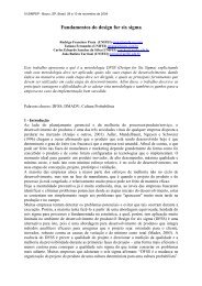
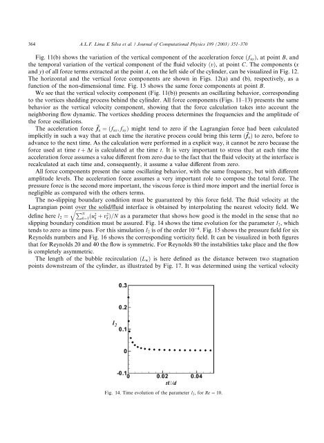
364 A.L.F. Lima E Silva et al. / Journal of Computational Physics 189 (2003) 351–370Fig. 11(b) shows the variation of the vertical component of the acceleration force ðf ay Þ, at point B, andthe temporal variation of the vertical component of the fluid velocity ðvÞ, at point C. The components (xand y) of all force terms extracted at the point A, on the left side of the cylinder, can be visualized in Fig. 12.The horizontal and the vertical force components are shown in Figs. 12(a) and (b), respectively, as afunction of the non-dimensional time. Fig. 13 shows the same force components at point B.We see that the vertical velocity component (Fig. 11(b)) presents an oscillating behavior, correspondingto the vortices shedding process behind the cylinder. All force components (Figs. 11–13) presents the samebehavior as the vertical velocity component, showing that the force calculation takes into account theneighboring flow dynamic. The vortices shedding process determines the frequencies and the amplitude ofthe force oscillations.The acceleration force ~ f a ¼ðf ax ; f ay Þ might tend to zero if the Lagrangian force had been calculatedimplicitly in such a way that at each time the iterative process could bring this term ð ~ f a Þ to zero, before toadvance to the next time. As the calculation were performed in a explicit way, it cannot be zero because theforce used at time t þ Dt is calculated at the time t. It is very important to stress that at each time theacceleration force assumes a value different from zero due to the fact that the fluid velocity at the interface isrecalculated at each time and, consequently, it assume a value different from zero.All force components present the same oscillating behavior, with the same frequency, but with differentamplitude levels. The acceleration force assumes a very important role to compose the total force. Thepressure force is the second more important, the viscous force is third more import and the inertial force isnegligible as compared with the others terms.The no-slipping boundary condition must be guaranteed by this force field. The fluid velocity at theLagrangian point qover ffiffiffiffiffiffiffiffiffiffiffiffiffiffiffiffiffiffiffiffiffiffiffiffiffiffiffiffiffiffiffiffiffiffiffithe solid/fluid interface is obtained by interpolating the nearest velocity field. WePdefine here l 2 ¼ Nk¼1 ðu2 k þ v2 k Þ=N as a parameter that shows how good is the model in the sense that noslipping boundary condition must be assured. Fig. 14 shows the time evolution for the parameter l 2 , whichtends to zero as time pass. For this simulation l 2 is of the order 10 4 . Fig. 15 shows the pressure field for sixReynolds numbers and Fig. 16 shows the corresponding vorticity field. It can be visualized in both figuresthat for Reynolds 20 and 40 the flow is symmetric. For Reynolds 80 the instabilities take place and the flowis completely asymmetric.The length of the bubble recirculation ðL w Þ is here defined as the distance between two stagnationpoints downstream of the cylinder, as illustrated by Fig. 17. It was determined using the vertical velocityFig. 14. Time evolution of the parameter l 2 , for Re ¼ 10.