The real options approach to valuation - Haskayne School of Business

The Real Op*ons Approach to Valua*on: Challenges and Opportuni*es Eduardo Schwartz UCLA Anderson School 2012 Alberta Finance Ins*tute Conference

Research on Real Op*ons Valua*on • Mines and Oil Deposits • Stochas*c Behavior of Commodity Prices • Forestry Resources • Expropria*on Risk in Natural Resources • Research and Development • Internet Companies • Informa*on Technology

Outline of Talk • Basic ideas about Real Op*ons Valua*on • Solu*on procedures • Natural resource investments and the stochas*c behavior of commodity prices • Research and Development Investments

Basic Ideas about Real Op*ons

Using Real Op*ons • Uncertainty and the firm’s ability to respond to it (flexibility) are the source of value of an op*on • When not to use real op*ons: – When there are no op*ons at all – When there is liXle uncertainty – When consequences of uncertainty can be ignored • Most projects are subject to op*ons valua*on

Investment Projects as Op*ons 1. Op*on to expand a project: Invest in a nega*ve NPV project which gives the op-on to develop a new project. 2. Op*on to postpone investment: Project may have a posi*ve NPV now, but it might not be op*mal to exercise the op-on to invest now, but wait un*l we have more informa*on in the future (valua*on of mines).

Investment Projects as Op*ons 3. Op*on to abandon: Projects are analyzed with a fixed life, but we always have the op-on to abandon it if we are loosing money. 4. Op*on to temporarily suspend produc*on: open and close facility.

Tradi*onal Valua*on Tools (DCF) • Require forecasts – A single expected value of future cash flows is generally used – Difficulty for finding an appropriate discount rate when op*ons (e.g., exit op*on) are present • Future decisions are fixed at the outset – no flexibility for taking decisions during the course of the investment project

Risk Neutral Valua*on • Lets first look at one aspect of the new approach • Tradi*onal vs. Certainty Equivalent approach to valua*on • Op*ons a liXle later

Tradi*onal Approach: NPV • Risk adjusted discount rateNPV=C0+N∑t = 1 (1 +Ctk)tC tin period t expected cash flow k risk adjusted discount rate

Certainty Equivalent Approach NPV=C0+N∑t = 1 (1 +CEQtr )ftCEQ tcertain cash flow that would be exchanged for risky cash flow (market based)

Simple Example • Consider a simplified valua*on of a Mine or Oil Deposit • The main uncertainty is in the commodity price and futures markets for the commodity exist (copper, gold, oil) • Brennan and Schwartz (1985) • For the moment neglect op*ons

Tradi*onal vs. CE Valua*on Tradi*onal Valua*on: NPV=C0+NNt t= + ∑t tCt0t= 1 (1 k)t=1 (1 +∑Rev−+CostqS−Costtk)tCertainty Equivalent Valua*on: NPV=C0+Nt tt = 1 (1 +∑qF− Costtr )ft

These Results are General Cox and Ross (1976), Harrison and Kreps (1979) and Harrison and Pliska (1981) show that the absence of arbitrage imply the existence of a probability distribu*on such that securi*es are priced at their discounted (at the risk free rate) expected cash flows under this risk neutral or risk adjusted probabili*es (Equivalent Mar-ngale Measure). Adjustment for risk is in the probability distribu*on of cash flows instead of the discount rate (Certainty Equivalent Approach).

• If markets are complete (all risks can be hedged) these probabili*es are unique. • If markets are not complete they are not necessarily unique (any of them will determine the same market value). • Futures prices are expected future spot prices under this risk neutral distribu*on. • This applies also when r is stochas*c. VT∫−rf ( t ) dt= EQ[ e0 0 XT]

Op*on Pricing Theory introduced the concept of pricing by arbitrage methods. • For the purpose of valuing op*ons it can be assumed that the expected rate of return on the stock is the risk free rate of interest. Then, the expected value of op*on at maturity (under the new distribu*on) can be discounted at the risk free rate. In this case the market is complete and the EMM is unique.

Using the Risk Neutral Framework to value projects allows us to • Use all the informa*on contained in futures prices when these prices exist • Take into account all the flexibili*es (op*ons) the projects might have • Use the powerful analy*cal tools developed in con*ngent claims analysis

Real Op*ons Valua*on (1) • Risk neutral distribu*on is known – Black Scholes world – Gold mine is, perhaps, the only pure example of this world F 0,T = S 0 (1+r f ) T

True and risk neutral stochas*c process for Gold prices dS= µ dt + σdzSdz ≈ N(0,dt)dS= rdt + σdz~Sdz ~ ≈ N(0,dt)

Real Op*ons Valua*on (2) • Risk neutral distribu*on can be obtained from futures prices or other traded assets – Copper mine, oil deposits • Challenges – Future prices are available only for short *me periods: in Copper up to 5 years – Copper mines can last 50 years! • The models fit prices and dynamics very well for maturi*es of available futures prices

Real Op*ons Valua*on (3) • Need an equilibrium model (CAPM) to obtain risk neutral distribu*on because there are no futures prices – R&D projects – Internet companies – Informa*on technology

Summary: Real Op*ons Valua*on • For many projects, flexibility can be an important component of value • The op*on pricing framework gives us a powerful tool to analyze those flexibili*es • The real op*ons approach to valua*on is being applied in prac*ce • The approach is being extended to take into account compe**ve interac*ons (impact of compe**on on exercise strategies)

Solu*on Procedures

Solu*on Methods (1) • Dynamic Programming approach – lays out possible future outcomes and folds back the value of the op*mal future strategy – binomial method • widely used of pricing simple op*ons • good for pricing American type op*ons • not so good when there are many state variables or there are path dependencies – Need to use the risk neutral distribu*on

Solu*on Methods (2) • Par*al differen*al equa*on (PDE) – has closed form solu*on in very few cases • BS equa*on for European calls – generally solved by numerical methods • very flexible • good for American op*ons • for path dependencies need to add variables • not good for problems with more than three factors • technically more sophis*cated (need to approximate boundary condi*ons)

Solu*on Methods (3) • Simula*on approach – averages the value of the op*mal strategy at the decision date for thousands of possible outcomes – very powerful approach • easily applied to mul*-­‐factor models • directly applicable to path dependent problems • can be used with general stochas*c processes • intui*ve, transparent, flexible and easily implemented – But it is forward looking, whereas op*mal exercise of American op*ons has features of dynamic programming

Valuing American Op*ons by Simula*on: A simple least-­‐squares approach • Longstaff and Schwartz, 2001 • An American op*on gives the holder the right to exercise at mul*ple points in *me (finite number). • At each exercise point, the holder op*mally compares the immediate exercise value with the value of con*nua*on. • Standard theory implies that the value of con*nua*on can be expressed as the condi*onal expected value of discounted future cash flows. 29

Valuing American Op*ons by Simula*on: A simple least-­‐squares approach • This condi*onal expecta*on is the key to being able to make op*mal exercise decisions. • Main idea of the approach is that the condi*onal expected value of con*nua*on can be es*mated from the cross-­‐sec*onal informa*on from the simula*on by least squares. 30

Valuing American Op*ons by Simula*on: A simple least-­‐squares approach • We es*mate the condi*onal expecta*on func*on by regressing discounted ex post cash flows from con*nuing on func*ons of the current (or past) values of the state variables. • The fiXed value from this cross-­‐sec*onal regression is an efficient es*mator of the condi*onal expecta*on func*on. It allows us to accurately es*mate the op*mal stopping rule for the op*on, and hence its current value.

Natural Resource Investments

Three Factor Model: Actual (Cortazar and Schwartz (2003)) dS=( ν − y) Sdt + σ11Sdzdy= −κ ydt +σ2dz 2( ν ν ) dt σ 3 dz 3dν= a − +

Three Factor Model: Risk Neutral dSdy( )∗ν − y − λ Sdt + σ=1 1Sdz1( )∗−κy− λ dt + σ= 2 2dz2( ν ν ) λ dt σ*dν= ( a − − + dz3 )33We need to make assumptions about the functionalform of the market prices of risks

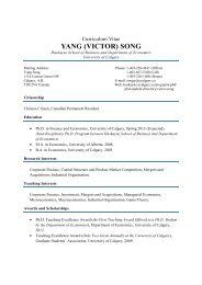
30.00Oil Futures 01/08/99Three-Factor Model25.0020.00Price (US$)15.00ObservedModel10.005.000.000 1 2 3 4 5 6 7 8 9 10Maturity (Years)

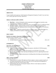
40Oil Futures 10/12/00Three-Factor Model3530ObservedModel25Price (US$)201510500 1 2 3 4 5 6 7 8 9 10Maturity (Years)

What to do for longer maturi*es? • Accept the model predic*ons for maturi*es where there are no futures prices? • Maybe a few years only? • Assume flat futures prices? • Assume futures prices increase at a fixed rate (infla*on?)? • Since there is more uncertainty in this area, what discount rate to use (risk free rate?)?

Recent work on Commodi*es • Two recent papers with Anders Trolle • “Unspanned stochas*c vola*lity and the pricing of commodity deriva*ves” (2009) • “Pricing expropria*on risk in natural resource contracts – A real op*ons approach” (2010)

NYMEX crude-­‐oil futures and op*on data • Largest and most liquid commodity deriva*ves market in the world • Largest range of maturi*es and strike prices, which vary significantly during the sample period • Daily data from Jan 2, 1990 to May 18, 2006 • We choose the 12 most liquid contracts for the analysis M1, M2, M3, M4, M5, M6 (first 6 monthly contracts) Q1, Q2 (next two quarterly contracts expiring in Mar, Jun, Sep or Dec) Y1, Y2, Y3, Y4 (next four yearly contracts expiring in Dec)

Evidence of unspanned stochas*c vola*lity • If we regress changes in vola*lity on the returns of futures contracts (or its PC), the R2 will indicate the extent to which vola*lity is spanned • But vola*lity is not directly observable • Return on Straddles: Call + Put with the same strike (closest to ATM); low “deltas” and high “vegas”. Model independent • Changes in log normal implied vola*li*es: average expected vola*lity over the life of the op*on

Procedure • We factor analyze the covariance matrix of the futures returns and retain the first three principal components (PCs) • Regress straddle returns (changes in implied vola*li*es) on PCs and PCs squared • We find that the R2 are typically very low, especially for the implied vola*lity regressions (between 0 and 21%)

Procedure • Thus, factors that explain futures returns cannot explain changes in vola*lity • We then factor analyze the covariance matrix of the residuals from these regressions. If there is unspanned stochas*c vola*lity in the data we should see large common varia*on in the residuals • We find that typically the first two PC explain over 80% of the varia*on in the residuals

Two Vola*lity Factors (SV2)

Pricing expropria*on risk in natural resource contracts • Conference on “The Natural Resources Trap, Private Investment without Public Commitment ” (Kennedy School, Harvard) • There are many dimensions to the study of expropria*on risk in natural resource investments: poli*cal, environmental, sociological, economic • In our approach we abstract from many of these issues and we concentrate on some of the important economic trade-­‐offs that arise from a government having an “op*on” to expropriate the resource

Expropria*on Op*on • We value a natural resource project, in par*cular an oil field, exposed to expropria*on risk • We view the government as holding an op*on to expropriate the oil field

Expropria*on Trade-­‐off • Government faces the following trade-­‐off in expropria*on (think about Argen*na vs YPF) – Benefit: • receives all profits rather than a frac*on through taxes – Costs: • Private firm may produce oil more efficiently • Government may have to pay compensa*on to the firm • Government faces “reputa*onal” costs

Assump*ons • We abstract from the various opera*onal op*ons that are typically embedded in natural resource projects and concentrate on the expropria*on op*on • Spot prices, futures prices and vola*li*es are described by the one vola*lity factor model (SV1)

Solu*on Procedure • Expropria*on op*on can be exercised at any *me during the life of the op*on: American-­‐style (LSM) • At every point in *me the government must compare the value of immediate exercise with the condi*onal expected value (under the risk neutral measure) of con*nua*on • Outcome is the op*mal exercise *me for each simulated path which can be used to value the expropria*on op*on • We can also es*mate the value of the oil field to the government and the firm both in the presence and absence of expropria*on risk

Main Results • For a given contractual arrangement the value of the expropria*on op*on increases with – The spot price – The slope of the futures curve (contango, backwarda*on) – The vola*lity of the spot (futures) price • For a given set of state variables the value of the expropria*on op*on decreases with the – Tax rate – Various expropria*on costs • The increase in the field’s value to the government due to expropria*on risk is always smaller than the decrease in the field value to the firms, since there are “deadweight losses” associated with expropria*on (produc*on inefficiency and “reputa*onal costs”)

R&D Investments Focus has been the pharmaceutical industryFramework, however, applies just as well toother research-intensive industries

R&D Investments • The pharmaceu*cal industry has become a research-­oriented sector that makes a major contribu*on to health care. • The success of the industry in genera*ng a stream of new drugs with important therapeu*c benefits has created an intense public policy debate over issues such as – the financing of the cost of research – the prices charged for its products – the socially op*mal degree of patent protec*on

• There is a trade-­‐off between promo*ng innova*ve efforts and securing compe**ve market outcomes. • The expected monopoly profits from drug sales during the life of the patent compensate the innovator for its risky investment. • The onset of compe**on aVer the expira*on of the patent limits the deadweight losses to society that arise from monopoly pricing under the patent. • Regula*on has had important effects on the cost of innova*on in the pharmaceu*cal industry.

Analysis of R&D projects is a very difficult investment problem • Takes a long *me to complete • Uncertainty about costs of development and *me to comple*on • High probability of failure (for technical or economic reasons) • Drug requires approval by the FDA • Uncertainty about level and dura*on of future cash flows • Abandonment op*on is very valuable

TuVs Center for the Study of Drug Development (December 2001) • Average development *me for new drugs: 12 years • Average total drug research costs (millions) Out-­‐of-­‐pocket expenses: Including cost of capital (11%): $802 – Calculated at *me of marke*ng of drug $403 – Includes cost of failed drugs (20% success) • More recent figures go up to $4 billion per drug • Yearly US expenditures in prescrip*on drugs :$308 billion (2010)

Research Spending Per New Drug Company Ticker Number ofdrugs approved R&D SpendingPer Drug ($Mil) Total R&DSpending1997-2011($Mil) AstraZeneca AZN 5 11,790.93 58,955 GlaxoSmithKline GSK 10 8,170.81 81,708 Sanofi SNY 8 7,909.26 63,274 RocheHolding AG RHHBY 11 7,803.77 85,841 Pfizer Inc. PFE 14 7,727.03 108,178 Johnson &Johnson JNJ 15 5,885.65 88,285 Eli Lilly & Co. LLY 11 4,577.04 50,347 AbbottLaboratories ABT 8 4,496.21 35,970 Merck & Co Inc MRK 16 4,209.99 67,360 Bristol-MyersSquibb Co. BMY 11 4,152.26 45,675 Novartis AG NVS 21 3,983.13 83,646 Amgen Inc. AMGN 9 3,692.14 33,229 Sources: InnoThink Center For Research In Biomedical Innovation; ThomsonReuters Fundamentals via FactSet Research Systems

Pfizer ‘Youth Pill’ Ate Up $71 Million Before It Flopped (WSJ: May 2, 2002) • The experimental drug aimed to reverse the physical decline that comes with aging. • Nearly a decade of research. • Pa*ents taking the frailty drug had gained some muscle mass – but less than 3% more than the placebo group – which also experienced muscle increase. • Drug appeared ineffec*ve.

Mediva*on, Pfizer end work on Alzheimer’s Drug (WSJ: January 18, 2012 • In 2008 Pfizer agreed to pay $225 million upfront – and up to $500 million if successful – for development rights to Dimebon. • Some 5.4 million in the US and 18 million worldwide are es*mated to have Alzheimer’s • Analysts say that effec*ve treatment could reach $25 billion per year

Success story: Lipitor from Pfizer • Most prescribed name-­‐brand in the US with 3.5 million people taking it every day • Enter the market in 1997 and loss patent protec*on at the end of Nov. 2011 with total sales of $81 billion • But (WSJ May 2, 2112), Pfizer's first-­‐quarter profit declined 19% as sales of its top product, Lipitor, tumbled 71% in the U.S. amid compe**on from generic copies.

R&D Valua*on 1. Evalua*on of Research and Development Investments (with M. Moon, 2000) 2. Patents and R&D as Real Op*ons (2004) 3. R&D Investments with Compe**ve Interac*ons (with K. Miltersen, 2004) 4. A Model of R&D Valua*on and the Design of Research Incen*ves (with J. Hsu, 2008)

Patents and R&D as Real Op*ons • Methodology for the valua*on of a single R&D project that is patent protected • Or equivalently, for determining the value of a patent to develop a par*cular product

Real Op*ons Approach • Treat the patent protected R&D project or the patent as a complex op*on on the variables underlying the value of the project – expected costs to comple*on – an*cipated cash flows • Uncertainty is introduced in the analysis by allowing these variables to follow stochas*c processes through *me • The risk adjusted process for the cash flows is obtained using the “beta” of traded pharmaceu*cal companies

Approach • R&D project takes *me to complete • Maximum rate of investment • Total cost to comple*on is random variable • Probability of failure (catastrophic events) • Op*on to abandon the project • When, and if, project is completed cash flows start to be generated • Cash flows are uncertain (level and dura*on) • Project is patent protected un*l *me T

Patent-protected R&D ProjectInvest K at rate IReceive CTerminal value0τT

Investment Cost Uncertainty Expected cost to comple*on follows (technical uncertainty): 2dK = −Idt+ σ ( IK)1dzVariance of cost to comple*on:~Var(K)=σ2K2 −σ22λ :Poisson Pr obabilityofFailure

Cash Flow Uncertainty Cash flow rate follows Geometric Brownian mo*on which may be correlated with cost process: dC= α Cdt +φCdwRisk adjusted process used for valua*on: dC= ( α −η)Cdt + φCdw= α * Cdt +φCdw

Value of Project once Investment has been Completed: V(C,t) 1 22φ C2VCC+ α * CV + V − rV + CCt=0Subject to boundary condi*on at expira*on of the patent: V( C,T)=M• CHas solu*on: CV ( C,t)= [1 − exp( −(r −α*)(T − t))]+ MC exp( −(r − *)( T − t))r −α*α

Stochas*c process for the (true) return on the project once investment is completed dVV= ( r +η ) dt + φdwVola*lity and risk premium are the same as for cash flows. Assuming the ICAPM holds the risk premium is: η = β ( r − r) m

Value of the Investment Opportunity: F(C,K,t) MaxI1 2 2 1 22[ φ C FCC+ σ ( IK)FKK+ φσρC(IK)2 2IF + F − ( r + λ)F − I]= 0Kt1FCK+ α * CFC−Subject to boundary condi*on at comple*on of investment: F ( C,0,τ ) = V ( C,τ )Problem with this is that *me of comple*on is random.

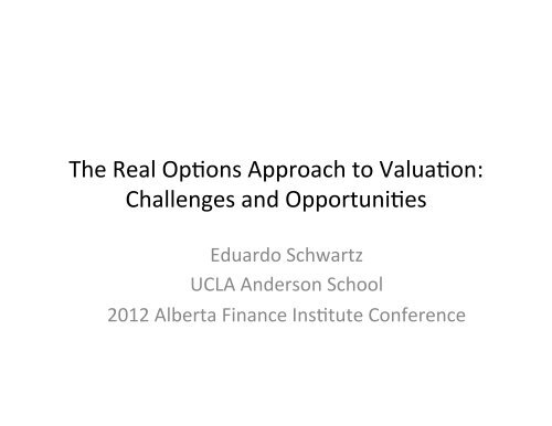
Figure 4:Critical Values for InvestmentCash Flow Rate18.0017.0016.0015.0014.0013.0012.0011.0010.009.00Invest at Maximum RateDo not InvestProject Value Equal 08.0080.00 85.00 90.00 95.00 100.00 105.00 110.00 115.00 120.00Cost to Completion

R&D Investments with Compe**ve Interac*ons (joint with K. Miltersen) • Concentrates on compe**ve interac*ons and the effect it has on valua*on and op*mal investment strategies • Real op*ons framework is extended to incorporate game theore*cal concepts • Two firms inves*ng in R&D for different drugs both targeted to cure the same disease • If both firms successful: Duopoly profits in marke*ng phase. But it can affect decisions in development phase. Decisions in development phase affects outcome in marke*ng phase

Compe**on in R&D projects • Compe**on brings about – Higher produc*on at lower prices – Higher probability of success – Shorter average development *me • But with higher total development costs and lower values to firms

A Model of R&D Valua*on and the Design of Research Incen*ves (joint with J. Hsu) • Malaria, Tuberculosis, and African strains of HIV kill more than 5 million people each year • Almost all of the death occur in the developing world • Very liXle private pharmaceu*cal investment devoted to researching vaccines for these diseases • A small market problem—people in the developing countries can’t afford to pay • Interna*onal organiza*ons and private founda*ons willing to provide funding (WHO, Gates Founda*on)

Current Literature on “Encouraging Pharmaceu*cal Innova*on” • Kremer (2001, 2002) review popular subsidy programs • Push programs: subsidize the cost of the R&D – Research grant – Co-­‐payment • Pull programs: subsidize the revenue of the R&D – Purchase commitment – Tax incen*ve – Extended patent protec*on

Current Literature • No analy*cal framework for contras*ng the different incen*ve programs The Contribu*on • Develop a real op*ons valua*on model for general R&D • Examine the different incen*ve programs quan*ta*vely using the valua*on framework

What’s new in this paper? • Quality of the R&D output is modeled explicitly • Revenue is a func*on of – the quality – the firm’s pricing (and quan*ty) strategy – Market demand • Firm’s price and quan*ty strategy could depend on – Incen*ve program in place – Monopoly power

Analyzing Incen*ve Contracts • Push Contracts: – Full discre*onary research grant – Sponsor co-­‐payment • Pull Contracts: – Extended patent protec*on – Fixed price purchase commitment – Variable price purchase commitment

Contract Specifics • Developer retains right, supplies monopoly quan*ty – Full discre*onary research grant – Sponsor co-­‐payment – Patent extension • Sponsor can contract the socially op*mal quan*ty to be produced – Purchase commitment contracts • We abstract from agency problem arising from asymmetric informa*on between vaccine developer and sponsor, and from contrac*ng issues

We seek to answer five cri*cal ques*ons • What is the required level of monetary incen*ve to induce the firm to undertake the vaccine R&D? • What are the expected price, quan*ty supplied and efficacy of the developed vaccine? • What is the probability that a viable vaccine will be developed? • What is the consumer surplus generated? • What is the expected cost per individual successfully vaccinated?