What to trust in a Magnetotelluric Model? - IGU

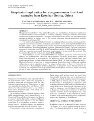
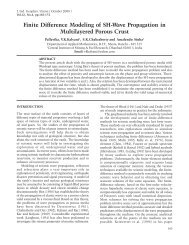
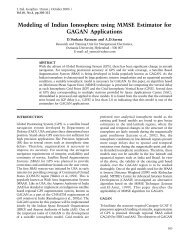
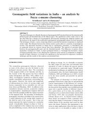
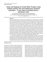
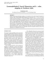
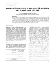
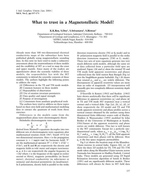
J. Ind. Geophys. Union ( Jan. 2004 )Vol.8, No.2, pp.157-171What to trust in a Magnetotelluric Model?K.K.Roy, S.Dey 1 , S.Srivastava 2 , S.Biswas 3Department of Geological Sciences, Jadavpur University, Kolkata - 700 0321Department of Geology and Geophysics, I.I.T., Kharagpur – 721 3022AFPRO, Ashok Nagar, Ranchi – 834 0063Schlumberger Asia, Mumbai – 400 086Already more than 500 two-dimensional electricalconductivity maps of the subsurface have beenpublished globally using magnetotelluric soundingdata. In this note we have tried to make a subjectiveassessment about the trustworthiness of these modelsand the credibility of MT as a tool to map the crustand upper mantle. Since many of the readers areapprehensive about the scientific viability of thesemodels, the responsibility lies with the MTcommunity to defend the scientific contents of thesemodels. The authors highlight the following pointsto address the topic.(A) Differences in the TE and TM mode models(B) Common features in these models(C) Repeatability of observation(D) Use of rotation invariant parameters(E) Data quality and signal strength(F) Purpose of investigation(G) Constraints from auxiliary geophysical toolsThe authors have tried to address on these topicsbased on their own field and mathematical modelingdata to extract the quantum of truth from theseexercises.Differences in the models came from themagnetotelluric plane wave electromagnetic theoryHelmholtz electromagnetic wave equationE E∇ 2 _____ = ν 2 _____HHderived from Maxwell’s equations decouples into twodifferent sets of electromagnetic wave equations aftermathematical rotation (Swift 1967; Vozoff 1972) fortwo-dimensional structures. Here ν is the propagationconstant (ν = √ iωµ(σ+iωε) for harmonic field), ∇ 2are the mathematical operator (∇ 2 = ∂ 2 /∂x 2 + ∂ 2 /∂y 2 +∂ 2 /∂z 2 ), and E and H are respectively the electric andmagnetic fields in volt/ meter and ampere turn/meter.ω, µ, σ & ε are respectively the angular frequency (ω=2πƒ where ƒ is the frequency of the signal in cycles/second or Hertz), magnetic permeability (in henry/meter), electrical conductivity (in mho/meter orseimens) and electrical permittivity (in farad/meter).In E-polarization, electric field is parallel to the strikedirection (transverse electric (TE) or E|| mode) and inH- polarization magnetic field is parallel to the strikedirection (transverse magnetic (TM) or E⊥ mode).These two sets of wave equations generate two verymuch different earth models, although the same setof data collected from a particular field spot areanalyzed. Figure 1(b) and (c) show the rotated TE andTM mode field apparent resistivities and phasescollected from the field station Baxi Barigah (Fig.1a)over the Singhbhum granite batholith. Fig.1 (b) showsthat rotated ρ axyand ρ ayxare widely different. Thediscrepancies in apparent resistivity values are morethan an order of magnitude. 1D interpretation willnaturally give two completely different resistivity depthsections.D’Erceville & Kunetz (1962) and Rankin (1962)have shown analytically that there will be significantdifference in apparent resistivities (ρ a) and phase (φ)in TE and TM mode MT responses near a verticalcontact and a vertical dyke. Figs 2(a), (b), (c), (d), (e)show respectively the 2D model and TE and TMmode apparent resistivity and phase profiles across avertical contact obtained by the authors using threedimensional finite difference source code of Mackie,Madden & Wannamaker (1993) modified by JohnBooker of the University of Washington at Seattle,USA.Nature of the apparent resistivity and phasecurves are widely different. This fact is well knownto the MT community. Except for a perfectly onedimensionalearth, where ρ axy= ρ ayx(ρ axy=1/ωµ 0⏐E x/H y⏐ 2 and ρ ayx= 1/ωµ 0⏐E y/H x⏐ 2 ), all the field apparentresistivities and their phases will be different. Hereµ 0is the free space magnetic permeability.Fig.3 (a) shows the location map of the Khandwa-Ujjain traverse in central India. Figures 3(b), (c), (d)show the three 2D models for TE, TM and TE+TMmode taken along the Khandwa-Ujjain traverse acrossNarmada-Son lineament in Madhya Pradesh, CentralIndia. These models are generated using 2D RapidRelaxation Inversion algorithm of Smith & Booker(1991) and are significantly different models. Thesedifferences will always be there in MT field data157

K.K.Roy et al.Figure 1. (a) Shows the location of the MT site Baxi Barigah in North-South Keonjhargarh profile, eastern India,(b) and (c) are respectively the magnetotelluric rotated TE and TM mode apparent resistivities and phases; apparentresistivity curves are showing more than an order of magnitude difference.158

What to trust in a Magnetotelluric Model?Figure 2 (a). Shows an earth model having the vertical contact EFHG parallel to the y-direction, the block ADFEILHGis having resistivity of 1 ohm-m., the block EBCFGJKH is having resistivity of 100 ohm-m, (b) and (c) show respectivelythe MT apparent resistivities and phases in TE mode across the vertical contact, (d) and (e) show respectively theMT apparent resistivities and phases in TM mode across the vertical contact.159

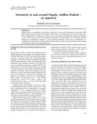
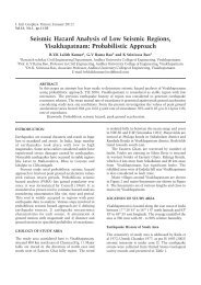
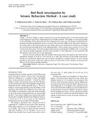
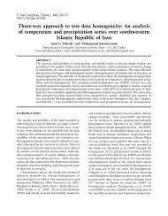
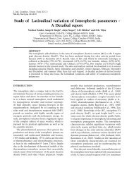
K.K.Roy et al.interpretation. We cannot choose one of these modelsas a true representative of the subsurface structure.Mathematical ModeL EXPERIMENTModel 1: Fig.4(a) shows a 3D model of a 100 km. cubeof resistivity 5000 ohm-m. with 3 graben type ofstructures. The dimensions of these three structuresare respectively given by (i) left graben : width 2km.,depth 40 km., resistivity of the rock filling the graben50 ohm.m, (ii) central graben : width 20 km. anddepth 25 km., resistivity of the rocks fiing the grabenis assumed to be 200 ohm-m. and (iii) right graben :width 1 km. and depth 30 km., resistivity of thematerial filling the graben is 10 ohm-m.Figs 4(b) and (c) show the TM and TE modeapparent resistivity pseudosections obtained from 3Dfinite difference source code of Mackie, Madden &Wannamaker (1993). The ordinate, time period, is inlog to the base 10 scale. The abscissa is distance inkilometer. The two apparent resistivity pseudosectionsshow that the TM mode apparent resistivities aresuperior to the TE mode apparent resistivities inresolving vertical faults, dykes etc.Model 2: Fig.5 (a) shows a model of a 100 km. cubeof resistivity 5000 ohm-m. Four dykes of width 100meters, depth extent 10 km. and mutual separationof 2km. between these dykes are assumed. Thesedykes are assumed at a depth of 500 meters from thesurface. Resistivity of the rocks filling the grabenstructures is assumed to be 20 ohm-m.Figs 5(b) and (c) show respectively the TE modeapparent resistivity and phase profile across thesedykes. Figs. 5(d) and (e) show the TM mode apparentresistivity and phase profiles across these dykes. Figs5(d) and (e) show that both TM mode apparentresistivity and phase profiles could resolve all the dykesseparately. TE mode apparent resistivity and phaseprofiles failed to resolve the presence of the four dykes.Model 3: Fig.6 (a) shows a 100 km. cube ofresistivity 5000 ohm-m. in which a conducting dykeof width 15 meter is assumed. Resistivity of thematerials filling the dyke is taken to be 10 ohm-m.and the depth of the dyke was varied from 15 m. to 1km. Figs 6(b) and (c) show the TM and TE modeprofiles across the dyke. The two figures clearly showthat TM mode MT has immensely superior resolvingpower than the TE mode MT. TE mode MT sees thetarget from a greater distance. As a result biggervolume of earth materials are involved in generatingthe TE mode response.These three sets of model experiments clearlyshow that the resolving power of the TM moderesponse is very much different from that of the TEmode response. Electric and magnetic fields paralleland perpendicular to the strike direction of thestructures reflect very much different physicalproperties of the earth. Discrepancies in these modelspartly come from theory and partly come from theinhomogeneities and anisotropies of the subsurface.Common features in the modelsStrong data with minimum noise content will alwaysshow some common features in all the models evenafter using different inversion source codes anddifferent MT parameters. Geometrical shapes of thesemajor features may be different. Some of the minorsignatures may be different in different modelsobtained from different magnetotelluric parameters. 2Dquantitative models should be accepted in asemiquantitative way and the broad features, whichare common in all the models, should be taken withgreater degree of confidence. If several earth modelshave something common, then earth must have thatproperty (Bachus & Gilbert 1967). All the three TE,TM and (TE+TM) models presented in the Figs 3b,c and d show the blackish high conductivity zone. Thegeometrical shapes of these zones are different indifferent models. All the three models show that thecontinent is rifted in this area. These parts arecommon in all the three models and can be acceptedFigure 3(a). Shows the location map of the Khandwa-Ujjain traverse.160

What to trust in a Magnetotelluric Model?Figure 3(b), (c) and (d) show respectively the TE, TM and TE+TM mode models of the Khandwa-Ujjain traverse.161

K.K.Roy et al.Figure 4(a). Shows three assumed grabens with different dimensions in a 100km. cube (not to scale) of resistivity5000 ohm-m.: (i) left graben is having a width of 2km., depth 40km. and filling material of resisitivity 50 ohm-m, (ii)central graben is having a width of 20km., depth 25km. and filling material of resistivity 200 ohm-m and (iii) rightgraben is having a width of 1km. depth 30km. and filling material of resistivity 10 ohm-m, (b) and (c) are respectivelythe TM and TE mode apparent resistivity pseudosections across the three assumed grabens in the model.162

What to trust in a Magnetotelluric Model?as reliable information. Other MT group (viz. NGRI,India group) who worked in this area also mapped thishigh conductivity zone with different geometricalshapes. Fig 7(a), (b) and (c) show the TE, TM andTE+TM mode models over the Singhbhum granitebatholith along the north-south traverse overKeonjhargarh, Orissa. All the three models areshowing black highly resistive Singhbhum granitebatholith. These parts can be trusted with greaterlevel of confidence. Whoever will run an MT traverseover the Singhbhum granite batholith will map thishighly resistive batholith. A highly conducting zone,delineated in TM and TE+TM mode models justbelow the resistive cover, is absent in TE mode model.We have seen in the previous section that verticalresolution in TM mode model is much better thanthat in TE mode model. Therefore some weightageis attached to the TM mode model but furtherverification from deep seismic sounding is necessarybefore we can confirm that it is a case of magmaticunderplating.Repeatability of observationsIf two interpretations are found to be more or lesssame from two independent field observations takenin different time, then one can trust those models.As for example, the authors found from twoindependent field studies that Singhbhum granitebatholith near Keonjhargarh is deep rooted; the depthextent of the batholith is 20km. or more and thegranite body (Roy, Singh & Rao 1998a), (SBGA Saha1994) is highly resistive. Roy, Singh & Rao (1998a),Roy, Mukherjee & Naskar (1996) have alreadymentioned that most highly resistive rocks in theArchaean craton of Singhbhum are Singhbhum granitephase II near Keonjhargarh and Older Metamorphicsnear Champua (oldest rock of India). Thereforerepeatability of observation enhances the credibility ofmodels.Use of rotation invariant magnetotelluric tensorsMagnetotelluric rotation invariant tensors are thosewhose amplitude remains constant after 360 0mathematical rotation (Vozoff 1972), (Swift 1967). Thefour-tensor elements in MT, viz, Zxx (=Ex/Hx), Zxy(=Ex/Hy), Zyx (=Ey/Hx) and Zyy (=Ey/Hy) describeellipses of the same size and ellipticity not onlytheoretically (Eggers 1982) but field observations alsoshow the same property (Fig 8a). Berdichevskii &Dmitriev (1976); Eggers (1982); Szarka & Menville(1997); Lilley (1993), Roy, Srivastava & Singh (1998b)have discussed about the properties of these rotationinvariant tensors. The authors have chosen only threepairs of these rotation invariant tensors and theirphases to propose that they generate much moretrustworthy models. The three pairs of rotationinvariant apparent resistivities and phases arerespectively given by:a) (i) ρ D= ⏐Z ΧΧZ ΥΥ- Z ΧΥZ ΥΧ⏐/ωµ(ii) φ D= phase of [Z ΧΧZ ΥΥ- Z ΧΥZ ΥΧ]b) (i) ρ B= ⎢Z B⎢ 2 /ωµwhere Z B= (Z xy- Z ΥΧ)/2(ii) φ B= phase of (Z xy- Z ΥΧ)/2c) (i) ρ C= ⎜Z C⎜ 2 /ωµ(ii) φ C= tan -1 (Υ/Χ)whereZ C= [X + iY]X = [(Zxx r+Zyy r) 2 + (Zxy r-Zyx r) 2 ] 1/2 / 2Y = [(Zxx i+Zyy i) 2 + (Zxy i-Zyx i) 2 ] 1/2 / 2r and i stands for the real and imaginary componentsof the impedance tensor element Z respectively.Fig.8 (b) shows the plots of field TE, TM and therotation invariant determinant, central and averageapparent resistivities. Whatever be the discrepancy orseparation between the TE and TM mode apparentresistivities, the rotation invariant ρ determinant(ρ D) ,ρ central(ρ C) and ρ average(ρ B) values are very close to each otherat all the periods. So the models they generate afterinversion are also very close to each other. Rotationinvariant apparent resistivities are approximatelytreated as 1D apparent resistivities. Therefore 2Dmodel based on 1D inversion should be done. In(ρ D,φ D) and (ρ C,φ C) pairs, information from real andimaginary components of all the four tensor elementsare present. The information content is more in theseparameters. Therefore they will generate moretrustworthy models in 1D, 2D and 3D domains. For2D however, TE and TM mode electromagnetic waveequations cannot be used for rotation invariantparameters. Therefore 2D model may be made basedon 1D inversion information.The idea of bringing rotation invariant parametersin modeling came from increasing the quantum ofinformation in the input data by introducing thediagonal elements of the impedance tensor. RoutineTE and TM mode impedances deal only with one offdiagonal element Zxy or Zyx. Increase in informationcontent reduces the differences between the basic dataand therefore reduces the discrepancies in the models.As a result reliability or confidence level of the modelswill increase in rotation invariance domain. Figs 9(a),(b) and (c) show the 2D models obtained from (ρ D,φ D),163

K.K.Roy et al.Figure 5(a). Shows a 100 km. cube (not to scale) of resistivity 5000 ohm-m. in which 4 dykes of width 100m. anddepth extents of 10km. are placed at a mutual separation of 2km. The resistivity of the filling material is 20 ohm-m.in all the dykes. MT traverse is taken at right angles to these four dykes along the x-direction, (b) and (c) arerespectively the TE mode apparent resistivity and phase profiles, (d) and (e) show respectively the TM mode apparentresistivity and phase profiles.164

What to trust in a Magnetotelluric Model?a)b)c)Figure 6(a). Shows a 100 km. cube of resistivity 5000 ohm-m. in which a dyke of width 15m. and resistivity 10 ohmm.is emplaced; depth extent of the dyke varies from 15m. to 1km, (b) and (c) show respectively the TM and TE modeapparent resistivity profiles across the assumed dyke in the model; the profile is at right angle to the strike direction.165

K.K.Roy et al.(ρ B,φ B) and (ρ C,φ C) using the questionable anddebatable TE mode part of 2D RRI. The models ofthe Khandwa- Ujjain traverse based on the rotationinvariant parameters are quite similar and are morereliable. Since the rotation invariant apparentresistivities are quite close, the models generated outof them will be similar in whatever way theinterpretation is done.Strength of the Noise and SignalTo increase the reliability of the earth models the dataquality should be good. The general guidelines theMT community follows are: (i) Avoid solar quiet daysand try to choose solar disturbance days for MT surveywhen the signals are strong, (ii) Avoid areas full ofcultural noise. Generally, high tension power lines,electrified railway tracks, defense installations,highways, underground cables destroy signals to aconsiderable extent at many places, (iii) Collection ofdata for extended periods i.e. for 15 to 30 days at aparticular spot improves the longer period data qualityand enhances the trustworthiness of the deeper partof the models and (iv) Strong signal improves the dataquality. The days before and after the magnetic stormsare preferable.Purpose of investigationField planning is very important to improve qualityof the models. Whether the investigation is formapping (i) lithosphere-asthenosphere boundary (ii)magma chambers in a volcanic cone (iii) high heat flowareas or (iv) sediments below the flood basalts, willdictate the field planning, which will dictate thequality of interpretation. For mapping lithosphereasthenosphereboundary with considerable clarities,granite batholiths or any hard rock areas should bechosen. Higher the resistivity of the upper crustalrocks, lesser will be the attenuation of the highfrequency MT signals, better will be the resolutionof the subsurface.An MT station over Cambay basin in India where3 to 4 kms. of Quaternary and Tertiary sedimentsoverlie Deccan basalts, most of the high frequency MTsignals will attenuate considerably in the highlyconducting sediments and only long period signalswith poorer resolving power will penetrate deep insidethe earth. Geoelectrical models, for mapping thelithosphere will always be more trustworthy if theobservations are taken over exposed granites/granodiorites or any other high-grade metamorphicterrain. Even granite windows do not guarantee bettermodels always. Higher conductivity of the lower crustcan reduce the detectibility of the Lithosphere-Asthenosphere boundary considerably. For mappinghorizontal boundaries TE and TM mode MT willbehave more or less in the same way. For a perfect1D structure the concept of TE and TM modevanishes and ρ axybecomes equal to ρ ayxat allfrequencies.If the purpose of investigation is to reach beyondolivine-spinel transition zone, then the signals mustbe recorded with period of upto 30,000 to 40,000seconds, if not more, with continuous observation of30 to 40 days together at a stretch and at one spot.TE and TM mode signals should be interpretedtogether. Some geomagnetic signals from thepermanent observatories should also be taken intoaccount.Electrical conductivity has very strong dependenceon the degree of partial melts and temperature(Shankland & Waff 1977). Since degree of partial meltand temperature increases with depth, electricalconductivity of the upper mantle silicates (garnetlherzolite) increases rapidly. As a result attenuationof the EM signals will also increase at a faster pace.Therefore MT models will suffer from resolutionproblem and only some broad major features will bereflected in these models at a depth of 300 to 450 km.from the surface. At a greater depth geomagnetic depthsounding (GDS) from a permanent observatory andearthquake seismological data should be interpretedto increase the reliability of the earth models obtainedfrom MT. At this depth TE and TM mode MT willbehave in a similar way for horizontal or nearlyhorizontal boundaries.Constraints from auxiliary geophysical toolsInformation from complementary geophysical toolswill always increase the reliability of the models.Therefore scientists attach more weightage on theintegration of the geophysical methods. Authors triedto use the information from gravity, seismic reflectionand heat flow survey to improve the quality ofinterpretation. Integration of information collectedfrom different geophysical tools improves reliabilityand acceptability of the models.CONCLUSIONSa) Magnetotelluric TE, TM and TE+TM models willhave some difference. It is difficult to choose one ofthe three as the true representative of the subsurface.Models obtained after quantitative interpretationshould be taken in a semiquantitative way. Common166

What to trust in a Magnetotelluric Model?Figure 7(a), (b) and (c) Show respectively the TE,TM and TE+TM mode models over the Singhbhum granite batholith,along the north-south traverse over Keonjhargarh, Orissa.167

K.K.Roy et al.Figure 8(a). Shows the traces of Zxx, Zxy, Zyx, Zyy, Zb, Zc in the complex domain; Zb, Zc are respectively the averageand central impedance tensors, (b) shows the TE and TM apparent resistivity curves along with the rotation invariantapparent resistivities over the station Baxi Barigah; Rd, Rb and Rc are respectively the determinant, average andcentral apparent resistivities.168

What to trust in a Magnetotelluric Model?Figure 9(a), (b) and (c) show respectively the 2D models of the Khandwa-Ujjain traverse obtained using rotationinvariant determinant, average and central apparent resistivity and phase and using the TE mode formulation of the2D RRI.169

K.K.Roy et al.features in all the models with different geometricalshapes should be accepted with greater level ofconfidence. Minor features which are not common inTE, TM and TE+TM mode models should preferablybe ignored or attached some weightage after crossverification from other auxiliary geophysical orgeological tools.b) From model experiment it has been shown veryclearly that for vertical inhomogeneities, viz., grabens,dykes, etc., TM mode MT anomalies are much moresharper than TE mode MT anomalies. Therefore,greater weightage can be attached to the TM modemodels for mapping shear zones, suture zones, faults,fractures, lineaments, etc.c) Rotation invariant apparent resistivities and theirphases are very close to each other. Moreover, theinformation content will be more in (ρ D,φ D), (ρ C,φ C)and (ρ B,φ B) pairs. Therefore, models generated fromrotation invariant parameters will be very close andmore trustworthy. For 1D and 3D problems we canuse these pairs as such for modeling. For 2D we haveto make 2D stiched in models from 1D-invertedmodels because TE and TM mode electromagneticwave equations cannot be used for rotation invariantparameters. Models generated using RITs and TE modeof RRI are presented just to show the readers how dothey look like.d) Routine do’s and don’ts in MT, which are wellknown to the MT community, must be followedreligiously to improve the trustworthiness of themodels. These guidelines are (i) avoid cultural noiseas far as practicable (ii) avoid solar quiet days as faras practicable for field measurements (iii) summermonths are preferable for MT field data acquisition(iv) for deeper probing, hard rock terrain should bechosen so that high frequency MT signals also canpenetrate to a considerable depth.e) For interpretation of MT data collected over anArchaean or Proterozoic terrain, if we go for 1Dinversion, we should over parameterize the models toincrease the trustworthiness of the models. 3 to 4layered earth model for a granite batholith or ahighgrade granulitic terrain is not acceptable to thegeologists. For 2 dimensional interpretation if wechoose square or rectangular blocks of bigger size infinite difference or finite element forward models,square elements or blocks of different colors appearin the 2D models. Geologists are reluctant to acceptthe square blocks in the models. Either very fine finitedifference cells should be taken with some increasein computation time or finite element method withisoparametric elements should be chosen to map thecomplicated subsurface geology.ACKNOWLEDGEMENTSAuthors are grateful to DST for sanctioning theproject ESS/16/103/98. Thanks are due to the DirectorGeneral of the Geological Survey of India for providinginfrastructural facilities for carrying out fieldwork nearKhandwa, Madhya Pradesh. Thanks are due to Mackiefor providing us their softwares for model experiment.Thanks are due to Mr.S.P.Hazra of IIT, Kharagpur fordrafting the diagrams nicely. Thanks are due to JohnBooker for allowing us to work with their softwares.REFERENCESBachus,G.E.& Gilbert, F., 1967. NumericalApplication of formalism for geophysical inverseproblems, Geophys. J.R. Astr. Soc., 13, 247-276.Berdichevskii, M.N. & Dmitriev, V.I.,1976. Basicprinciples of interpretation of magnetotelluriccurves in geoelectric and geothermal studies,KAPG geophysical monograph, pp.165-221, ed.Adam, A., Academic Kiado, Budapest.D’ Erceville, L. & Kunetz, G., 1962. The effect of afault on the earth’s natural electromagnetic Field,Geophysics, 27, 666-676.Eggers, D.E.,1982. An eigen state formulation of themagnetotelluric impedance tensor, Geophysics,47,1204-1214.Lilley, F.E.M., 1993. Magnetotelluric analysis usingMohr Circle. Geophysics, 58, 1498-1506.Mackie,R.L., Madden,T.R. & Wannamaker,T.E., 1993,Three Dimensional Magnetotelluric Modellingusing difference equations-Theory andComparison to Integral Equation Solution,Geophysics, 58, 215-226.Rankin, D., 1962. The magnetotelluric effect on aDike, Geophysics, 27, 651-665.Roy, K. K., Singh, A. K. & Rao, C. K., 1998a. Twodimensional Magnetotelluric model of theSinghbhum granite batholith. in DeepElectromagnetic Exploration, pp.120.-151, Eds.Roy, K.K., Verma, S.K. & Mallick, K., SpringerVerlag, Germany.Roy, K. K., Srivastava, S. & Singh, A. K., 1998b.Rotation invariant magnetotelluric impedancetensor: a case study from West Singhbhum,Bihar, in Deep Electromagnetic Exploration, pp.99-119, Eds. Roy, K.K., Verma, S.K. & Mallick,K., Springer Verlag, Germany.Roy, K.K., Das, L. K., Mukherjee, K. K. & Naskar,D. C.,1996. Some upper crustal information ofthe Singhbhum craton based on direct currentgeoelectric survey. Indian Journal of Geology170

What to trust in a Magnetotelluric Model?(Special Issue Saha Volume), 71, 1-2, 133-142.Saha, A.K., 1994. Crustal evolution of Singhbhumnorth Orissa Eastern India, Mem., 27, Geol. Soc.Ind., Bangalore, 341P.Shankland,T.J. & Waff, H.S.,1977. Partial melting andelectrical conductivity anomalies in the uppermantle, J.Geophys.Res., 82 (33),5409-5417Smith, J. T. & Booker, J.R., 1991. Rapid RelaxationInversion of two and three dimensionalmagnetotelluric data, J. Geophys. Res., 96(B3),3905-3922.Swift, C.M., 1967. A magnetotelluric investigation ofan electrical conductivity anomaly in the southwestern United States, Ph.D. thesis, M.I.T.,Cambridge, MA, USA. Magnetotelluric Methods,SEG publication, Ed. Vozoff, K., 156-166.Szarka,L. & Menvielle, M., 1997, Analysis of rotationalinvariants of the magnetotelluric impedance,Geophys. J. R. Astr.l Soc., 129, 133-142.Vozoff, K., 1972. The magnetotelluric method in theexploration of sedimentary basins, Geophysics,37, 98-141.(Accepted 2003 September 24. Received 2003 September 23; in original form 2003 February 22).171