Implementing a Class of Structural Change Tests - Institute for ...

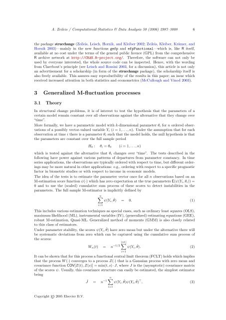
A. Zeileis / Computational Statistics & Data Analysis 50 (2006) 2987–3008 6the package strucchange (Zeileis, Leisch, Hornik, and Kleiber 2002; Zeileis, Kleiber, Krämer, andHornik 2003)—mainly in the new functions gefp and efpFunctional—which is, like R itself,available at no cost under the terms of the general public licence (GPL) from the comprehensiveR archive network at http://CRAN.R-project.org/. Therefore, the software can not only beused by everyone interested, the whole source code can be inspected. Hence, with the wordingfrom Claerbout’s principle (see Leisch and Rossini 2003, for a discussion), this article is not onlyan advertisement for a scholarship (in form of the strucchange package), the scholarship itself isalso freely available. This assures easy reproducibility of the results in this paper; an issue whichreceived increased attention in both statistics and econometrics (McCullough and Vinod 2003).3 Generalized M-fluctuation processes3.1 TheoryIn structural change problems, it is of interest to test the hypothesis that the parameters of acertain model remain constant over all observations against the alternative that they change over“time”.More formally, we have a parametric model with k-dimensional parameter θ i for n ordered observationsof a possibly vector-valued variable Y i (i = 1, . . . , n). Under the assumption that for eachobservation at time i there is a parameter θ i such that the model holds, the null hypothesis is thatthe parameters are constant over the full sample periodH 0 : θ i = θ 0 (i = 1, . . . , n)which is tested against the alternative that θ i changes over “time”. The tests described in thefollowing have power against various patterns of departures from parameter constancy. In timeseries applications, the observations are typically ordered with respect to time, but different orderingsmay be more natural in other applications: e.g., ordering with respect to a specific prognosticfactor in biometric studies or with respect to income in economic models.The idea of the tests is to estimate the parameter vector once for all n observations based on anM-estimation score function ψ(·) which has zero expectation at the true parameters E(ψ(Y i , θ i )) =0 and to use the (scaled) cumulative sum process of these scores to detect instabilities in theparameters. The full sample M-estimator is implicitly defined byn∑ψ(Y i , ˆθ) = 0. (1)i=1This includes various estimation techniques as special cases, such as ordinary least squares (OLS),maximum likelihood (ML), instrumental variables (IV), (generalized) estimating equations (GEE),robust M-estimation, Quasi-ML. Generalized method of moments (GMM) is also closely relatedto this class of estimators.Under parameter stability, the scores ψ(Y i , ˆθ) have zero mean but under the alternative there willbe systematic deviations from zero which can be captured using the cumulative sum process ofthe scores:⌊nt⌋∑W n (t) = n −1/2 ψ(Y i , ˆθ). (2)It can be shown that for this process a functional central limit theorem (FCLT) holds which impliesthat the process W (·) converges to a process Z(·) that is a Gaussian process with zero mean andcovariance function COV[Z(t), Z(s)] = min(t, s) · J, where J is the (asymptotic) covariance matrixof the scores ψ. Usually, this covariance structure can easily be estimated, the simplest estimatorbeing∑ nĴ = n −1 ψ(Y i , ˆθ)ψ(Y i , ˆθ) ⊤ , (3)i=1i=1Copyright © 2005 Elsevier B.V.