Untitled - Bedales Schools

More documents

Recommendations

Info

effectively a single species model with the rate of change of population being proportional to thepopulation at that instant. Thus the rate of change of population at time t is given byd N= rN ⇒ Nn() t = N (0)e,d twhere the constant r, the coefficient of growth, depends upon the number of births and deaths.Hence the population grows at an exponential rate. Such a situation is unreal for most species, withmany factors affecting growth. The human population, however, demonstrates such a growth overthe past three hundred years.Adolphe Quetelet is regarded as one of the founders of statistics. He understood the national importanceof demography and, in 1826, published data on mortality rates in Brussels, dividing them intogroups by age and sex. He influenced Verhulst, who in 1836 proposed a self-limiting process forpopulations growing large, as opposed to the Malthusian model. Quetelet proposed that he shouldconsider a quantity opposing population growth, rather like friction opposing motion. He proposed acarrying capacity, k, such thatd Nd t⎛ N ⎞= rN ⎜ 1 − ⎟ ,⎝ k ⎠where N is the population at time t and r is a positive constant. Verhulst used the term logistique inhis 1845 paper [6] and the term ‘logistic curve’ is associated with Verhulst’s work. The logisticcurve would be used to read off populations at specified times. The solution to the differential equationabove is known as the logistic equation. Much debate followed as to whether this could beregarded as a law of nature. Verhulst himself remained realistic, realising that the model dependedentirely upon the choice of function as ‘resistance to growth’. The general acceptance of the logisticequation in the early part of the 20th century owes much to the almost crusading enthusiasm of RaymondPearl. He was the main protagonist in the United States, where the equation evolved independently.Pearl and Reed introduced the same curve in 1920, following on from the work of Robertson,a physiologist. Like Verhulst, Pearl realised that something beyond a quantitative resemblance wasnecessary to establish the equation as a law. The validity of the logistic equation as a law dependedon its accuracy in predicting the known data on population levels. They predicted a limiting figure of197 million as the population of the USA and gave the point of inflection of the curve to the exactday (1 April 1914). They were less than successful when applying the logistic curve to the populationsof other nations. Pearl was joined by Lotka, who proposed models of the type dN/dt = aN + bN 2 .Unlike Pearl, Lotka realised the limits of the logistic equation as a law of nature.One of the main contributors to the mathematical theory of population growth was the Italian mathematicianVolterra. His background was quite different from the biological and statistical fields ofVerhulst and Pearl. Schooled in the analysis of Dini and the mathematical physics of Betti, Volterrabrought a different approach to the problem. In 1925 Volterra began to consider the variations in twopopulations inhabiting the same environment [7]. He became interested in the problem when askedto provide a mathematical explanation for the varying fish populations in the Adriatic during the FirstWorld War.Volterra considered predator–prey models. He considered populations N 1 and N 2 , in which the firstdoubles in time t 1 and the second halves in time t 2 . He then supposed that the populations inhabit thesame environment and that the first population preys on the second population. He formed thegrowth rates of the two populations asdNdtdN= ( a − b N ) N and = ( − a + b N ) N ,dt1 21 2 2 1 2 2 1 240
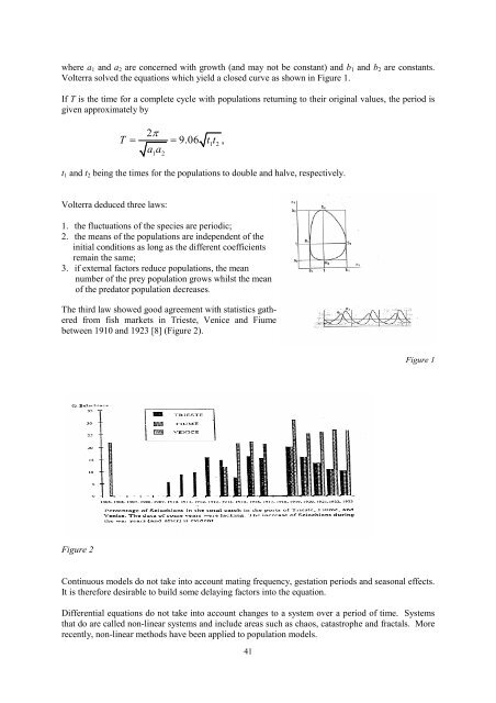
where a 1 and a 2 are concerned with growth (and may not be constant) and b 1 and b 2 are constants.Volterra solved the equations which yield a closed curve as shown in Figure 1.If T is the time for a complete cycle with populations returning to their original values, the period isgiven approximately by2πT = = 9.06 t1t2,aa1 2t 1 and t 2 being the times for the populations to double and halve, respectively.Volterra deduced three laws:1. the fluctuations of the species are periodic;2. the means of the populations are independent of theinitial conditions as long as the different coefficientsremain the same;3. if external factors reduce populations, the meannumber of the prey population grows whilst the meanof the predator population decreases.The third law showed good agreement with statistics gatheredfrom fish markets in Trieste, Venice and Fiumebetween 1910 and 1923 [8] (Figure 2).Figure 1Figure 2Continuous models do not take into account mating frequency, gestation periods and seasonal effects.It is therefore desirable to build some delaying factors into the equation.Differential equations do not take into account changes to a system over a period of time. Systemsthat do are called non-linear systems and include areas such as chaos, catastrophe and fractals. Morerecently, non-linear methods have been applied to population models.41
Page 2 and 3: Contents:An Interview with Harry Pe
Page 4 and 5: The Bedales Science Magazine
Page 6 and 7: An Interview with Harry PearsonCan
Page 8 and 9: 6-2 Physics Trip to CERN, Genevaver
Page 10 and 11: The Final Century?t the end of Worl
Page 12 and 13: Spring at the North Polehere’s a
Page 14 and 15: PC hazards and the lawHAZARDOUS WAS
Page 16 and 17: Incinerators are some of the larges
Page 18 and 19: IJoseph Rotblatfind myself writing
Page 20 and 21: Many resins are brittle and unstabl
Page 22 and 23: RECYCLINGThe reprocessing of plasti
Page 24 and 25: and processed to drinking water sta
Page 26 and 27: Interview with Professor Tony Marmo
Page 28 and 29: Finally, what should Bedales be doi
Page 30 and 31: Hydrogen Fuel Cell Car(We built one
Page 32 and 33: • Less land needed for landfill s
Page 34 and 35: The Science of the Sune know very l
Page 36 and 37: The 6-1 Physics Trip to Thorpe Park
Page 38 and 39: Stem Cell Researchlthough medicine
Page 40 and 41: The potential for technological adv
Page 42 and 43: How Aspirin Worksrostaglandins are
Page 46 and 47: References and notes:[1] Roy Porter
Page 48: The B-Sci CrosswordAcross1. The pro

Untitled - Bedales Schools

Create successful ePaper yourself

Delete template?

Save as template?