A Chaotic RC Oscillator

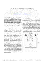
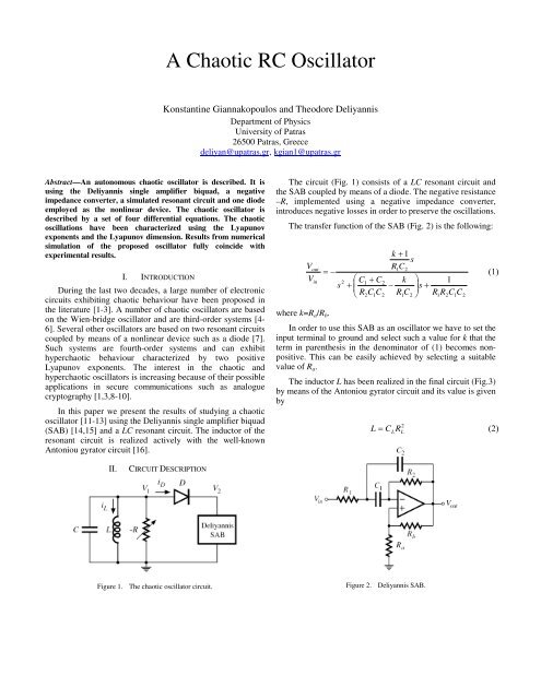
A Chaotic RC OscillatorKonstantine Giannakopoulos and Theodore DeliyannisDepartment of PhysicsUniversity of Patras26500 Patras, Greecedeliyan@upatras.gr, kgian1@upatras.grAbstract—An autonomous chaotic oscillator is described. It isusing the Deliyannis single amplifier biquad, a negativeimpedance converter, a simulated resonant circuit and one diodeemployed as the nonlinear device. The chaotic oscillator isdescribed by a set of four differential equations. The chaoticoscillations have been characterized using the Lyapunovexponents and the Lyapunov dimension. Results from numericalsimulation of the proposed oscillator fully coincide withexperimental results.I. INTRODUCTIONDuring the last two decades, a large number of electroniccircuits exhibiting chaotic behaviour have been proposed inthe literature [1-3]. A number of chaotic oscillators are basedon the Wien-bridge oscillator and are third-order systems [4-6]. Several other oscillators are based on two resonant circuitscoupled by means of a nonlinear device such as a diode [7].Such systems are fourth-order systems and can exhibithyperchaotic behaviour characterized by two positiveLyapunov exponents. The interest in the chaotic andhyperchaotic oscillators is increasing because of their possibleapplications in secure communications such as analoguecryptography [1,3,8-10].In this paper we present the results of studying a chaoticoscillator [11-13] using the Deliyannis single amplifier biquad(SAB) [14,15] and a LC resonant circuit. The inductor of theresonant circuit is realized actively with the well-knownAntoniou gyrator circuit [16].The circuit (Fig. 1) consists of a LC resonant circuit andthe SAB coupled by means of a diode. The negative resistance–R, implemented using a negative impedance converter,introduces negative losses in order to preserve the oscillations.The transfer function of the SAB (Fig. 2) is the following:VVinwhere k=R a /R b .s2⎛ C1+ C+⎜⎝ R2C1C22k + 1sR Ck ⎞ 1− sR1C⎟ +2 ⎠ R1R2C1C2out1 2= −(1)In order to use this SAB as an oscillator we have to set theinput terminal to ground and select such a value for k that theterm in parenthesis in the denominator of (1) becomes nonpositive.This can be easily achieved by selecting a suitablevalue of R a .The inductor L has been realized in the final circuit (Fig.3)by means of the Antoniou gyrator circuit and its value is givenbyL = C R 2(2)L LII.CIRCUIT DESCRIPTIONFigure 1. The chaotic oscillator circuit.Figure 2. Deliyannis SAB.

Then, the above set of differential equations (3) takes theform of the following fourth-order system:•x = αx − z − c(x − y −1)H ( x − y −1)•⎛ g ⎞y = kbhy − e⎜h + g + ⎟w− khc(x − y −1)H ( x − y −1)⎝ k ⎠•z = x•w = kbhy − e(h + g)w − khc(x − y −1)H ( x − y −1)(6)where H(u) is the Heaviside function, that isFigure 3. The final circuit.The negative resistor has been realized by a negativeimpedance converter circuit [15].III.NONLINEAR ANALYSISThe chaotic oscillator can be described by a set of fourdifferential equations. These equations derived easily from thecircuit (Fig. 3) are as follows:diLdV1V1V1 = L C + iL+ + iD= 0dt dt − RV2⎛ dV2dV3⎞ ⎛ dV2dVo⎞iD= + C1⎜− ⎟ + C2⎜− ⎟R1⎝ dt dt ⎠ ⎝ dt dt ⎠Ra⎛ dV2dV3⎞ V3−VV3= VoC1⎜− ⎟ =R + R ⎝ dt dt ⎠ Rabwhere i D is the current in the diode. Assuming a piecewiselinear model for the diode we have2o(3)⎧ 0 , V1−V2−VD< 0⎪iD= ⎨V1−V2−V(4)D⎪, V1−V2−VD≥ 0⎩ rDwhere r D and V D are the diode forward biased resistance andthe diode voltage drop respectively.In order to modify the above equations in a wayconvenient for numerical analysis we introduce the followingnotation:V1x =VDtθ =τρc =rDV2y =VD•duu =dθρe =R2ρiLz =VDLρ =CCg =C1V3w =VDρα =RCh =C2τ =LCρb =R1Rak =Rb(5)IV.⎧0,u < 0H ( u)= ⎨(7)⎩1,u ≥ 0CONFIRMATION OF CHAOSThe stability properties of the above continuousautonomous system have been studied by calculating theLyapunov exponents (LEs) and the Lyapunov dimension[13,17-19]. The LEs are defined by1λi= lim lnσi( t)(8)t →∞t} n i( ti=1if the limit exists. { σ ) are the eigenvalues of the system.Let λ 1 ≥ … ≥ λ n be the LEs of a dynamic system, and j bethe largest integer such that λ 1 +…+λ j ≥ 0. The Lyapunovdimension D L , as defined by Kaplan and Yorke [20], is asfollows:DLj+1j∑λiλ1 + ... + λji=1= j + = j +λλThe LEs measure the rate at which nearby trajectoriesconverge or diverge. There are as many LEs as there aredimensions of the system in the state space, but the largestexponent is the most important. If the largest LE is negative,then the trajectories converge in time and the system isinsensitive to initial conditions. If the largest LE is positive,then the distance between nearby trajectories growsexponentially in time and the system exhibits dependence oninitial conditions. For an attractor, contraction must outweighexpansion so the sum of all LEs has to be negative. For eachtrajectory, which does not terminate at a fixed point, at leastone LE vanishes [21]. If the attractor is an equilibrium point,all the LEs are negative and D L =0. If the attractor is a limitcycle, there exists one zero LE and the other LEs are negative,while D L =1. In case there is a two-torus, it has another LEzero while the other LEs are negative and D L =2. If it is a K-torus, it has K zero LEs and the other LEs are negative andD L =K, where K is an integer. In case it is chaotic, it has onej+1(9)

positive LE and the Lyapunov dimension is noninteger. If ithas two positive LEs, it is hyperchaotic.The LEs and Lyapunov dimension of the set of equations(6) have been calculated for various values of the parameter αand for a large number of iterations by means of LyapunovExponents Toolbox (LET) [22], which runs on MATLAB.They are shown in Figs. 4 to 7.Figure 7. Lyapunov dimension.It can be seen that the system exhibits a chaotic behaviourin the range of α from 0.15 to 0.25 and especially for α=0.20.The fourth LE (Fig. 6) is deeply negative.Figure 4. Largest Lyapunov exponent.V. SIMULATION AND EXPERIMENTAL RESULTSWe have simulated the circuit in Fig. 3 as well as built it inthe laboratory. For the LC resonant circuit we have selected afrequency of 1.5kHz implemented with C=61.9nF,C L =180.8nF and R L =1kΩ (corresponding to L=180.8mH). Theopamps UA741 and the diode 1N4148 with V D =0.65V andr D =25Ω at 5mA were used. The negative resistance wasimplemented with R′=5.6kΩ and a POT of 20kΩ.For the design of the SAB [14,15] we assume C 1 =C 2 andr=R 1 /R 2 . Then we taker1R = R2=2πfoC12πfoC1rRk =Ra1≥b2r(10)Figure 5. Three larger Lyapunov exponents.Optimizing the above SAB [15] we assume r=12.5⋅10 -6 ⋅f o .Selecting C 1 =C 2 =10nF and a frequency f o =800Hz we takeR 1 =1.99kΩ and R 2 =199kΩ. For the value of k we selectk=0.022 implemented with R b =100.1kΩ and R a by means of aPOT of 5kΩ.Figure 6. Fourth Lyapunov exponent.Figure 8. Phase portrait (i L against V 1).

Figure 9. Phase portrait (V 3 against V 1).Figure 12. Phase portrait (V 3 against i L).There is very good agreement between the PSPICE andMATLAB simulation and the experimental results.Figure 10. Phase portrait (V 3 against V 2).Figure 13. Time waveforms of chaotic variables V 1(t) and V 2(t).Figure 11. Phase portrait (i L against V 2).The oscillator has been simulated by means of MATLABsetting k=0.022, α=0.20, b=0.86, c=68.4, e=0.0086 andg=h=6.2. The correctness of our simulations has beenconfirmed also by means of PSPICE and Dynamics Solver[23]. Results are depicted in figures 8 to 16.Figure 14. Time waveforms of chaotic variables i L(t) and V 3(t).

Figure 15. 3D Phase portrait (i L against V 1 and V 2).Figure 16. 3D Phase portrait (i L against V 2 and V 3).VI.CONCLUSIONSAn autonomous chaotic oscillator using the DeliyannisSAB has been presented. It has been shown that it exhibitschaotic behaviour characterized by a positive Lyapunovexponent and large noninteger Lyapunov dimension. Theoscillator has been implemented in the laboratory as an activeRC circuit and was simulated by means of PSPICE andMATLAB.REFERENCES[1] “Special issue on chaos in nonlinear electronic circuits - part A:tutorials and reviews,” IEEE Trans. Circuits Syst.-I, vol. 40, pp. 640-786, 1993.[2] “Special issue on chaos in nonlinear electronic circuits - part B:bifurcations and chaos,” IEEE Trans. Circuits Syst.-I, vol. 40, pp. 792-884, 1993.[3] “Special issue on chaos in nonlinear electronic circuits - part C:applications,” IEEE Trans. Circuits Syst.-II, vol. 40, pp. 596-701, 1993.[4] A. Namajūnas and A. Tamaševičius, “ Modified Wien-bridge oscillatorfor chaos,” Electron. Lett., vol. 31, pp. 335-336, 1995.[5] A. S. Elwakil and A. M. Soliman, “A family of Wien-type oscillatorsmodified for chaos,” Int. J. Circ. Theor. Appl., vol. 25, pp. 561-579,1997.[6] A. Tamaševičius, G. Mykolaitis and A. Čenys, “Wien-bridge chaoticcircuit with comparator,” Electron. Lett., vol. 34, pp. 606-608, 1998.[7] A. Tamaševičius, A. Čenys, G. Mykolaitis, A. Namajūnas and E.Lindberg, “Hyperchaotic oscillator with gyrators”, Electron. Lett., vol.33, pp. 542-544, 1997.[8] M. Hasler, “Synchronization principles and applications,” IEEECircuits and Systems Tutorials, pp. 314-327, 1994.[9] “Special issue on chaos synchronization, control, and applications,”IEEE Trans. Circuits Syst.-I, vol. 44, pp. 856-1039, 1997.[10] “Special issue on communications, information processing and controlusing chaos,” Int. J. Theor. Appl., vol. 27, pp. 527-645, 1999.[11] K. Giannakopoulos, T. Deliyannis and J. Hadjidemetriou, “Means fordetecting chaos and hyperchaos in nonlinear electronic circuits,” Proc.14 th Int. Conf. DSP, Santorini, Greece, pp. 951-954, 2002.[12] K. Giannakopoulos, “Study and implementation of nonlinear electroniccircuits: chaotic oscillators, applications, jump phenomenon,” PhDThesis, Univ. of Patras, 2003.[13] K. Giannakopoulos and T. Deliyannis, “A comparison of five methodsfor studying a hyperchaotic circuit,” Int. J. Electron., vol. 92, pp. 143-159, 2005.[14] T. Deliyannis, “High-Q factor circuit with reduced sensitivity”,Electron. Lett., vol. 4, pp. 577-578, 1968.[15] T. Deliyannis, Y. Sun and J. K. Fidler, “Continuous-Time Active FilterDesign,” CRC Press LLC, 1999.[16] A. Antoniou, “Realization of gyrators using operational amplifiers andtheir use in RC-active-network synthesis,” Proc. IEE, vol. 116, pp.1838-1850, 1969.[17] T. S. Parker and L. O. Chua, “ Chaos: a tutorial for engineers,” Proc.IEEE, vol. 75, pp. 982-1008, 1987.[18] A. A. Tsonis, “Chaos – From Theory to Applications,” Plenum Press,New York, 1992.[19] R. C. Hilborn, “Chaos and Nonlinear Dynamics: An Introduction forScientists and Engineers,” Oxford Univ. Press, New York, 2000.[20] P. Frederickson, J. L. Kaplan, E. D. Yorke and J. A. Yorke, “TheLiapunov dimension of strange attractors,” J. Diff. Eq., vol. 49, pp.185-207, 1983.[21] H. Haken, “At least one Lyapunov exponent vanishes if the trajectoryof an attractor does not contain a fixed point,” Phys. Lett., vol. 94A, pp.71-72, 1983.[22] S. W. K. Siu, “Lyapunov Exponents Toolbox,” City Univ. of HongKong, 1998.[23] J. M. Aguirregabiria, “Dynamics Solver ver. 1.74,” Univ of the BasqueCountry, 2008.