ch3 random variables and distributions.pdf - Unix.eng.ua.edu

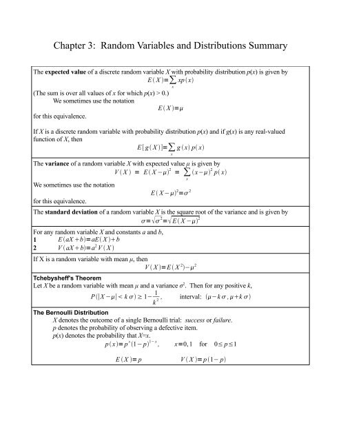
Chapter 3: Random Variables and Distributions SummaryThe expected value of a discrete random variable X with probability distribution p(x) is given byE X =∑ xp xx(The sum is over all values of x for which p(x) > 0.)We sometimes use the notationE X =for this equivalence.If X is a discrete random variable with probability distribution p(x) and if g(x) is any real-valuedfunction of X, thenE [ g X ]=∑ g x p xxThe variance of a random variable X with expected value μ is given byV X = E X − 2= ∑ x− 2 p xxWe sometimes use the notationE X − 2 = 2for this equivalence.The standard deviation of a random variable X is the square root of the variance and is given by= 2 = E X − 2For any random variable X and constants a and b,1 E aX b=aE X b2 V aX b=a 2 V X If X is a random variable with mean μ, thenV X =E X 2 − 2Tchebysheff's TheoremLet X be a random variable with mean μ and a variance σ 2 . Then for any positive k,P ∣X −∣ k ≥ 1− 1k 2 ,interval: −k ,k The Bernoulli DistributionX denotes the outcome of a single Bernoulli trial: success or failure.p denotes the probability of observing a defective item.p(x) denotes the probability that X=x.px= p x 1− p 1− x , x=0, 1 for 0≤ p≤1E X = pV X = p 1− p

A random variable Y possesses a binomial distribution if the following conditions are satisfied:1. The experiment consists of a fixed number n of identical trials.2. Each trial can result in one of only two possible outcomes, called success or failure.3. The probability of success p is constant from trial to trial.4. The trials are independent.5. Y is defined to be the number of successes among the n trials.The Binomial DistributionY denotes the number of successes in n trials.p denotes the probability of a success on any one given trial.p y= n1− p n− y , y=0,1,... ,n for 0≤ p≤1y pyE Y =npV Y =np1− pThe Geometric DistributionY denotes the number of the trial on which the first success occurs.p y= p1− p y−1 , y=1,2,... for 0 p1E Y = 1 V Y = 1− ppp 2The Negative Binomial DistributionY denotes the number of the trial on which the r th success occurs.p y= y−1r−1 pr 1− p y−r , y=r , r1, ... for 0 p1E Y = r r1− pV Y =pp 2The Poisson DistributionY denotesλ denotes the mean (use λt for more than one time interval, where t is the number of intervals).The Moment Generating Functionp y= yy! e− , y=0,1,2,...E Y = V Y =M t=E e tY