A Note on Cubic Convolution Interpolation - Biomedical Imaging ...

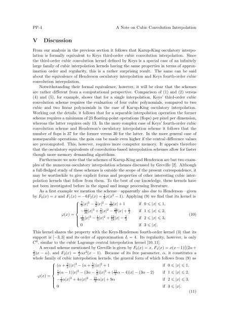
PP-4A <strong>Note</strong> on Cubic Convolution InterpolationVDiscussionFrom our analysis in the previous section it follows that Karup-King osculatory interpolationis formally equivalent to Keys third-order cubic convolution interpolation. Sincethe third-order cubic convolution kernel defined by Keys is a special case of an infinitelylarge family of cubic interpolation kernels having the same properties in terms of approximationorder and regularity, this is a rather surprising result. The same can be saidabout the equivalence of Henderson osculatory interpolation and Keys fourth-order cubicconvolution interpolation.Notwithstanding their formal equivalence, however, it will be clear that the schemesare rather different from a computational perspective. Comparison of (1) and (2) versus(4) and (5), for example, shows that for a single interpolation, Keys’ third-order cubicconvolution scheme requires the evaluation of four cubic polynomials, compared to twocubic and two linear polynomials in the case of Karup-King osculatory interpolation.Working out the details, it follows that for a separable interpolation operation the formerscheme requires a minimum of 23 floating-point operations (flops) per pixel per dimension,whereas the latter requires only 13. In the more complex case of Keys’ fourth-order cubicconvolution scheme and Henderson’s osculatory interpolation scheme it follows that thenumber of flops is 37 for the former versus 30 for the latter. In the more general case ofnonseparable operations, the gain can be made even higher if the central difference valuesare precomputed. This, however, requires more computer memory. It appears thereforethat the osculatory equivalents of convolution-based interpolation schemes allow for fasterthough more memory demanding algorithms.Furthermore we note that the schemes of Karup-King and Henderson are but two examplesof the numerous osculatory interpolation schemes discussed by Greville [2]. Althougha full-fledged study of these schemes is outside the scope of the present correspondence, itmay be worthwhile to give explicit forms and properties of other interesting cubic interpolationkernels that follow from them. To the best of our knowledge, these kernels havenot been investigated before in the signal and image processing literature.As a first example we mention the scheme—apparently also due to Henderson—givenby F 0 (x) =x and F 1 (x) =−6F 2 (x) = 1 6 x(x2 − 1). Applying (9) we find that its kernel is⎧⎪⎨ϕ(x) =⎪⎩79 |x|3 − 3 2 |x|2 − 518|x| +1 if 0 |x| 1,− 1136 |x|3 + 7 4 |x|2 − 28 9 |x| + 5 3if 1 |x| 2,136 |x|3 − 1 4 |x|2 + 1318 |x|− 2 3if 2 |x| 3,0 if 3 |x|.This kernel shares the property with the Keys-Henderson fourth-order kernel (3) that itssupport is [−3, 3] and its order of approximation L = 4. Its regularity, however, is onlyC 0 , similar to the cubic Lagrange central interpolation kernel [10, 11].A second scheme mentioned by Greville is given by F 0 (x) =x, F 1 (x) =x(x − 1) ( (2α +12 )x − α) ,andF 2 (x) = 1 2 αx2 (x − 1). Because of its free parameter, α, it constitutes awhole family of cubic interpolation kernels, the general form of which follows from (9) as⎧(α + 3 2 )|x|3 − (α + 5 2 )|x|2 +1 if 0 |x| 1,⎪⎨ 12ϕ(x) =(α − 1)|x|3 − (3α − 5 2 )|x|2 +( 11 2α − 4)|x|−(3α − 2) if 1 |x| 2,− 1 2⎪⎩α|x|3 +4α|x| 2 − 21 2α|x| +9α if 2 |x| 3,0 if 3 |x|.(11)(10)