INTERPRETATION OF AXIAL PILE LOAD TEST RESULTS FOR ...

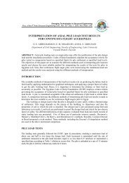
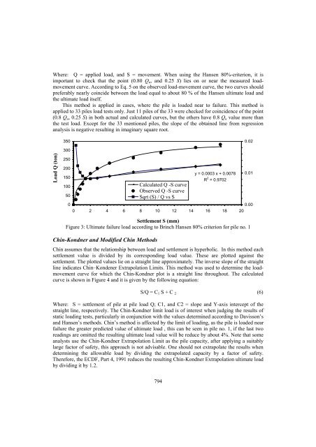
Where: Q = applied load, and S = movement. When using the Hansen 80%-criterion, it is
important to check that the point (0.80 Qu, and 0.25 S) lies on or near the measured loadmovement
curve. According to Eq. 5 on the observed load-movement curve, the two curves should
preferably nearly coincide between the load equal to about 80 % of the Hansen ultimate load and
the ultimate load itself.
This method is applied in cases, where the pile is loaded near to failure. This method is
applied to 33 piles load tests only. Just 11 piles of the 33 were checked for coincidence of the point
(0.8 Qu, 0.25 S) in both actual and calculated curves, but the others have 0.8 Qu value more than
the test load. Except for the 33 mentioned piles, the slope of the obtained line from regression
analysis is negative resulting in imaginary square root.
Load Q (ton)
350
300
250
200
150
100
50
0
Calculated Q -S curve
Observed Q -S curve
Sqrt (S) / Q vs S
794
y = 0.0003 x + 0.0078
R 2 = 0.9702
0 2 4 6 8 10 12 14 16 18 20
Settlement S (mm)
Figure 3: Ultimate failure load according to Brinch Hansen 80% criterion for pile no. 1
Chin-Kondner and Modified Chin Methods
Chin assumes that the relationship between load and settlement is hyperbolic. In this method each
settlement value is divided by its corresponding load value. These are plotted against the
settlement. The plotted values lie on a straight line approximately. The inverse slope of the straight
line indicates Chin–Kondener Extrapolation Limits. This method was used to determine the loadmovement
curve for which the Chin-Kondner plot is a straight line throughout. The calculated
curve is shown in Figure 4 and it is given by the following equation:
0.02
0.01
0.00
S/Q = C1 S + C 2 (6)
Where: S = settlement of pile at pile load Q; C1, and C2 = slope and Y-axis intercept of the
straight line, respectively. The Chin-Kondner limit load is of interest when judging the results of
static loading tests, particularly in conjunction with the values determined according to Davisson’s
and Hansen’s methods. Chin’s method is affected by the limit of loading, as the pile is loaded near
failure the greater predicted value of ultimate load , this can be seen in pile no. 1, if the last two
readings are omitted the resulting ultimate load value will be reduce by about 4%. Note that some
analysts use the Chin-Kondner Extrapolation Limit as the pile capacity, after applying a suitably
large factor of safety, this approach is not advisable. One should not extrapolate the results when
determining the allowable load by dividing the extrapolated capacity by a factor of safety.
Therefore, the ECDF, Part 4, 1991 reduces the resulting Chin-Kondner Extrapolation ultimate load
by dividing it by 1.2.