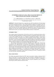
INTERPRETATION OF AXIAL PILE LOAD TEST RESULTS FOR ...

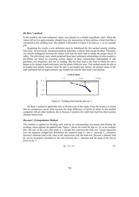
De Beer’s method
In this method, the load–settlement values were plotted on a double logarithmic chart. When the
values fall on two approximately straight lines, the intersection of these defines a limit load that is
considered a pile yielding load. The method is illustrated in Figure 6 for pile no. 1, as an example
pile.
Regarding the results a new definition must be introduced for this method namely yielding
limit load. All previously mentioned methods determine a failure load except De Beer. Therefore,
one should distinguish between the failure load and the limit load to adopt the proper factor of
safety. The pile failure load, which predicted from load–settlement relationships of piles loaded to
pre-failure are based on assuming certain shapes of these relationships independent of pile
geometry, soil properties, and rate of loading. But the limit load is the load at which the curve
begins to be steeper sloped and enters into the plastic behavior zone. This method needs the pile to
be loaded near failure, because when the pile is not loaded near failure, the plotted values of the
load settlement fall on approximately one straight line and the limit load is not defined.
Settlement S (mm)
0.1
Figure 6: Yielding limit load for pile no. 1
De Beer’s method is applicable only to 49 pile tests in this study. From the results it is found
that no comparison can be done because the large difference of factor of safety in this method
compared with all other methods, this is because it predicts the yield limit load but others predict
ultimate failure load.
Decourt’s Extrapolation Method
1
10
100
Load Q (mm)
1 10 100 1000
This method is applied by dividing each load by its corresponding movement and plotting the
resulting values against the applied load. Figure 7 shows the result for pile no. 26, as an example
pile. The part of the curve that tends to a straight line intersects the load axis. Linear regression
over the apparent straight-line determines the required slope C1 and y- intercept C2 constants.
Decourt’s ultimate load is the value at the intersection with the load axis, Decourt’s ultimate load
Qu can be accurately calculated as the ratio between the y- intercept and the slope of the line as
given in Eq. 7.
Qu = C2 / C1 (7)
796
Limit load =143