Forming Binary Near-Earth Asteroids From Tidal Disruptions

AbstractTitle of Dissertation:Forming Binary Near-Earth AsteroidsFrom Tidal DisruptionsKevin J. Walsh, Doctor of Philosophy, 2006Dissertation directed by:Professor Derek C. RichardsonDepartment of AstronomyWe present simulations and observations as part of a model of the binary near-Earthasteroid population. The study of binary asteroid formation includes a series of simulationsof near-Earth asteroid (NEA) tidal disruption, analyzed for bound, mutually orbitingsystems. Discrete and solid particles held together only by self-gravity are employed tomodel a “rubble pile” asteroid passing Earth on a hyperbolic encounter. This is accomplishedvia N-body simulations, with multiple encounter and body parameters varied. Weexamine the relative binary production rates and the physical and orbital properties ofthe binaries created as a function of the parameters. We also present the overall relativelikelihoods for possible physical and dynamical properties of created binaries.In order to constrain the shape and spin properties of the bodies that feed the NEApopulation, an observing campaign was undertaken to observe lightcurves of small MainBelt asteroids (D < 5 km, SMBAs). Observations of 28 asteroids increases the overallnumber of SMBAs studied via lightcurves to 86. These observations allow direct comparisonbetween NEAs and MBAs of a similar size.The shape and spin for the SMBAs are incorporated into a Monte Carlo model of asteady-state NEA population, along with the binaries created by tidal disruption simulations.Effects from tidal evolution and binary disruption from close planetary encountersare included as a means of altering or disrupting binaries. We find that with the bestknown progenitor (small Main Belt asteroids) shape and spin distributions, and current

estimates of NEA lifetime and encounter probabilities, that tidal disruption should accountfor approximately 1–2% of NEAs being binaries. Given the observed estimate ofan ∼ 15% binary NEA fraction, we conclude that there are other formation mechanismsthat contribute significantly to this population.

Forming Binary Near-Earth AsteroidsFrom Tidal DisruptionsbyKevin J. WalshDissertation submitted to the Faculty of the Graduate School of theUniversity of Maryland at College Park in partial fulfillmentof the requirements for the degree ofDoctor of Philosophy2006Advisory Committee:Professor Derek C. Richardson, advisorProfessor Michael F. A’HearnProfessor William D. DorlandProfessor Douglas P. HamiltonProfessor M. Coleman MillerProfessor Andrew S. Rivkin

c○ Kevin J. Walsh 2006

PrefaceMuch of the work in this dissertation is published, or in the process of being published.Chapter 2 appeared in the planetary-science journal Icarus, in nearly the same form aspresented here (Walsh & Richardson 2006). The work in Chapter 4 was recently submittedto the same journal, and is under review. Together, and with the results from Chapter3, this dissertation presents an ongoing study into the binary NEA population. As a wholeit provides details on the role that tidal disruption plays in creating the binary NEA population,and builds a framework for further studies in this field.Over the course of these studies the known population of binary asteroids in the SolarSystem has more than doubled. New discovery techniques have been used, and oldtechniques have been applied to different populations. Because of the rapidly changinglandscape, this work is quite timely and relevant to the latest observations and theoreticalwork being done. Beyond the answers provided about tidal disruption, the steady-statemodel will be able to incorporate new binary formation mechanisms as they become betterunderstood.ii

To all those who helped along the way...iii

AcknowledgementsI would not have made it to this point in my education without significantamounts of help and inspiration along the way. I would like to thank as manyas possible, starting with everyone at YMCA Camp Eberhart, where I firstlearned to use a telescope. Prof. Rettig at Notre Dame helped me immenselyby directing my first research projects and by keeping me working at theobservatory. Thanks to Derek for supplying plenty of freedom and supportas my advisor throughout my time at Maryland, from my second year projectall the way through to my dissertation. He never hesitated to send me to aconference or a telescope, and always encouraged my numerous side projects,which substantially enhanced my educational experience. I also owe manythanks to the faculty, staff and students at Maryland for making my timehere both fun and enriching. Thanks to the UMD-KPNO collaboration forsupplying me with observing time and funding in support of my dissertation.iv

ContentsList of TablesList of Figuresviiiix1 Introduction 11.1 Scientific Motivation . . . . . . . . . . . . . . . . . . . . . . . . . . . . 11.1.1 Why binary asteroids are interesting . . . . . . . . . . . . . . . . 11.1.2 Binary near-Earth asteroids . . . . . . . . . . . . . . . . . . . . . 21.1.3 Binary Main-Belt asteroids . . . . . . . . . . . . . . . . . . . . . 61.2 Binary Formation Mechanisms . . . . . . . . . . . . . . . . . . . . . . . 91.2.1 Capture . . . . . . . . . . . . . . . . . . . . . . . . . . . . . . . 121.2.2 Collisions . . . . . . . . . . . . . . . . . . . . . . . . . . . . . . 121.2.3 Rotational disruption . . . . . . . . . . . . . . . . . . . . . . . . 141.3 Shape and Spin Distributions for NEAs and MBAs . . . . . . . . . . . . 171.3.1 Existing lightcurve data . . . . . . . . . . . . . . . . . . . . . . 171.3.2 Recent studies . . . . . . . . . . . . . . . . . . . . . . . . . . . 181.3.3 Motivation for work on small MBAs . . . . . . . . . . . . . . . . 191.4 Steady-State Models of the NEA Population . . . . . . . . . . . . . . . . 201.4.1 Near-Earth asteroid population dynamics . . . . . . . . . . . . . 211.5 Background . . . . . . . . . . . . . . . . . . . . . . . . . . . . . . . . . 221.5.1 Tidal disruption . . . . . . . . . . . . . . . . . . . . . . . . . . . 221.5.2 Rubble piles . . . . . . . . . . . . . . . . . . . . . . . . . . . . 241.6 This Dissertation . . . . . . . . . . . . . . . . . . . . . . . . . . . . . . 252 Formation of Binary Asteroids via Tidal Disruption of Rubble Piles 262.1 Overview . . . . . . . . . . . . . . . . . . . . . . . . . . . . . . . . . . 262.2 Method . . . . . . . . . . . . . . . . . . . . . . . . . . . . . . . . . . . 272.2.1 Simulations . . . . . . . . . . . . . . . . . . . . . . . . . . . . . 272.2.2 Progenitors . . . . . . . . . . . . . . . . . . . . . . . . . . . . . 272.2.3 Tidal encounters and initial conditions . . . . . . . . . . . . . . 302.2.4 Analysis . . . . . . . . . . . . . . . . . . . . . . . . . . . . . . 32v

2.3 Results and Discussion . . . . . . . . . . . . . . . . . . . . . . . . . . . 332.3.1 Bulk results . . . . . . . . . . . . . . . . . . . . . . . . . . . . . 332.3.2 T-PROS and T-EEBs . . . . . . . . . . . . . . . . . . . . . . . . 452.3.3 Classes of disruption . . . . . . . . . . . . . . . . . . . . . . . . 472.3.4 3 h spin rate subset . . . . . . . . . . . . . . . . . . . . . . . . . 472.3.5 Triples and hierarchical systems . . . . . . . . . . . . . . . . . . 502.3.6 Tidal evolution and eccentricity damping . . . . . . . . . . . . . 502.4 Conclusion . . . . . . . . . . . . . . . . . . . . . . . . . . . . . . . . . 553 Lightcurve Observations of Small Main Belt Asteroids 573.1 Overview . . . . . . . . . . . . . . . . . . . . . . . . . . . . . . . . . . 573.2 Observations . . . . . . . . . . . . . . . . . . . . . . . . . . . . . . . . 583.3 Data Reduction and Photometry . . . . . . . . . . . . . . . . . . . . . . 603.3.1 Phase dispersion minimization . . . . . . . . . . . . . . . . . . . 613.4 Results and Discussion . . . . . . . . . . . . . . . . . . . . . . . . . . . 623.4.1 Well-determined lightcurves . . . . . . . . . . . . . . . . . . . . 633.4.2 Detections with significant constraints . . . . . . . . . . . . . . . 643.4.3 Marginal detections . . . . . . . . . . . . . . . . . . . . . . . . . 663.4.4 Spin and shape properties among small MBAs and NEAs . . . . . 743.5 Conclusions . . . . . . . . . . . . . . . . . . . . . . . . . . . . . . . . . 784 Steady-State Model of the Binary Near-Earth Asteroid Population 804.0.1 Previous work . . . . . . . . . . . . . . . . . . . . . . . . . . . 814.1 Steady-State Model . . . . . . . . . . . . . . . . . . . . . . . . . . . . . 834.1.1 Initial shape and spins . . . . . . . . . . . . . . . . . . . . . . . 834.1.2 NEA lifetimes and planetary encounters . . . . . . . . . . . . . . 844.1.3 Binary evolution . . . . . . . . . . . . . . . . . . . . . . . . . . 884.1.4 Migrating binary MBAs . . . . . . . . . . . . . . . . . . . . . . 924.2 Steady-State Results and Discussion . . . . . . . . . . . . . . . . . . . . 954.2.1 Nominal case . . . . . . . . . . . . . . . . . . . . . . . . . . . . 954.2.2 Influence of MBA binary percentage . . . . . . . . . . . . . . . . 964.2.3 Influence of MBA shape/spin properties . . . . . . . . . . . . . . 1014.2.4 Influence of tidal evolution . . . . . . . . . . . . . . . . . . . . . 1014.2.5 Estimates on the properties of binary NEAs formed by tidal disruption. . . . . . . . . . . . . . . . . . . . . . . . . . . . . . . 1034.2.6 Estimates of migrated binaries’ numbers and properties . . . . . . 1044.2.7 Doublet craters . . . . . . . . . . . . . . . . . . . . . . . . . . . 1054.3 Conclusion . . . . . . . . . . . . . . . . . . . . . . . . . . . . . . . . . 1055 Conclusions 1085.1 Future Work . . . . . . . . . . . . . . . . . . . . . . . . . . . . . . . . . 109vi

A Parameter Tests 113A.1 Bulk Density of Progenitor . . . . . . . . . . . . . . . . . . . . . . . . . 113A.2 Resolution of Progenitor . . . . . . . . . . . . . . . . . . . . . . . . . . 115A.3 Packing Efficiency of Progenitor . . . . . . . . . . . . . . . . . . . . . . 116A.4 Conclusions on Parameter Tests . . . . . . . . . . . . . . . . . . . . . . 118Bibliography 121vii

List of Tables1.1 Binary NEA properties. . . . . . . . . . . . . . . . . . . . . . . . . . . . 51.2 Binary MBA properties. . . . . . . . . . . . . . . . . . . . . . . . . . . 112.1 Binary formation statistics. . . . . . . . . . . . . . . . . . . . . . . . . . 333.1 Diameter estimates from H. . . . . . . . . . . . . . . . . . . . . . . . . . 593.2 Orbital, physical and lightcurve parameters for all targets. . . . . . . . . . 684.1 Lifetimes for binary NEAs. . . . . . . . . . . . . . . . . . . . . . . . . 904.2 Binary fractions for all simulations. . . . . . . . . . . . . . . . . . . . . 103A.1 Number of binaries produced at varying resolutions. . . . . . . . . . . . 116viii

List of Figures1.1 Binary NEA and MBA properties. . . . . . . . . . . . . . . . . . . . . . 102.1 Initial spin and shape parameters. . . . . . . . . . . . . . . . . . . . . . . 292.2 Distribution of v ∞ for NEA close encounters. . . . . . . . . . . . . . . . 312.3 Snapshots of a tidal disruption. . . . . . . . . . . . . . . . . . . . . . . . 322.4 Probability of binary formation for each parameter. . . . . . . . . . . . . 342.5 Binaries formed compared to mass of the largest remnant. . . . . . . . . . 362.6 Binary orbital properties. . . . . . . . . . . . . . . . . . . . . . . . . . . 382.7 Binary size ratio, obliquity and spin period. . . . . . . . . . . . . . . . . 412.8 Primary body shape statistics. . . . . . . . . . . . . . . . . . . . . . . . . 432.9 T-PROS and T-EEBs . . . . . . . . . . . . . . . . . . . . . . . . . . . . 462.10 Comparison of S-, B-, and M-class disruptions. . . . . . . . . . . . . . . 482.11 Spin periods of 3 h spin subset. . . . . . . . . . . . . . . . . . . . . . . . 492.12 Tidal evolution of semi-major axis. . . . . . . . . . . . . . . . . . . . . . 532.13 Eccentricity damping timescales. . . . . . . . . . . . . . . . . . . . . . . 543.1 Lightcurve plots . . . . . . . . . . . . . . . . . . . . . . . . . . . . . . . 693.2 Lightcurve plots . . . . . . . . . . . . . . . . . . . . . . . . . . . . . . . 703.3 Lightcurve plots . . . . . . . . . . . . . . . . . . . . . . . . . . . . . . . 713.4 Lightcurve plots . . . . . . . . . . . . . . . . . . . . . . . . . . . . . . . 723.5 Lightcurve plots . . . . . . . . . . . . . . . . . . . . . . . . . . . . . . . 733.6 Shape and spin distributions for different sized MBAs . . . . . . . . . . . 753.7 NEA and SMBA lightcurve distribution comparison . . . . . . . . . . . . 763.8 NEA and SMBA lightcurve distribution comparison, H < 17 . . . . . . . 774.1 Lightcurves periods and amplitudes for NEAs, MBAs and SMBAs . . . . 854.2 NEA lifetimes . . . . . . . . . . . . . . . . . . . . . . . . . . . . . . . . 864.3 Test of 3-body simulations . . . . . . . . . . . . . . . . . . . . . . . . . 914.4 MBA binary properties . . . . . . . . . . . . . . . . . . . . . . . . . . . 944.5 Number of binaries in nominal simulation . . . . . . . . . . . . . . . . . 974.6 Properties of binaries in nominal simulation . . . . . . . . . . . . . . . . 984.7 Lifetimes of binaries in nominal simulation . . . . . . . . . . . . . . . . 99ix

4.8 Percentage of migrated binaries . . . . . . . . . . . . . . . . . . . . . . . 1004.9 Influence of tidal evolution on simulations . . . . . . . . . . . . . . . . . 1025.1 Preliminary YORP spinup results . . . . . . . . . . . . . . . . . . . . . . 111A.1 Results from simulations with varying resolution. . . . . . . . . . . . . . 117x

Chapter 1Introduction1.1 Scientific Motivation1.1.1 Why binary asteroids are interestingThe discovery and observation of binary asteroids over the past decade has provided newways to study the properties of Solar System bodies. Before the 1993 discovery of Ida’scompanion Dactyl in the main asteroid belt by the Galileo mission, there were only unconfirmeddetections and theoretical speculation about binary asteroids. The inventory ofbinary minor planets has now eclipsed 100, there are known triple and even quadruplesystems, and detailed radar shape models are being produced for some nearby binaries(see Richardson & Walsh 2006 for a review). Of particular interest for this dissertationare binaries in the Main-Belt and near-Earth populations.The reason astronomers have searched for binary asteroids since the discovery of (1)Ceres is that binary asteroids can provide extensive insight into the physical properties ofthe bodies. They can also provide information about past and present dynamics affectingsmall bodies in the inner Solar System. A binary system typically allows for estimation1

of the system mass M by way of Kepler’s Third Law,P 2 = 4π 2 a 3 /GM (1.1)with period P and mean separation a typically directly measured, and G is the gravitationalconstant. In most situations component sizes and shapes can be modeled allowingfor a rare measurement of asteroid density. When coupled with a spectroscopic estimateof asteroidal composition, estimates on porosity and internal structure can be made.The dynamical mechanisms affecting various populations of small bodies can also bestudied by way of binary asteroids. Binaries have been discovered in nearly every dynamicalpopulation of minor planets, with large numbers among trans-Neptunian objects (orKuiper Belt Objects), one binary Jovian Trojan, two binary Centaurs, and a plethora ofbinary Main Belt and near-Earth asteroids. Adding to this inventory are recent discoveriesof complex systems such as the additional satellites of Pluto, a triple KBO 2003 EL 61 ,and a triple Main-Belt asteroid (MBA) system (87) Sylvia. Since each population boastsdramatically different dynamical, collisional and thermal environments, the existence anddetailed study of binaries will be quite valuable.1.1.2 Binary near-Earth asteroidsThe known binary near-Earth asteroids (NEAs) have been discovered from a combinationof lightcurve and radar observations. Lightcurve studies, where an asteroid’s magnitudeis plotted over time, have been conducted on a large number of bodies. However, certainorbital properties (asynchronous orbit and favorable geometry) are needed to make anunambiguous assessment of the state of the binary (Weidenschilling et al. 1989; Pravec& Hahn 1997). The secondaries must be large enough (∼20% of the primary) for theirnonsynchronous periods to be observed above any noise in the lightcurve of the primaries.Observations must also capture occultations/eclipses over multiple revolutions of the sec-2

ondary body, which requires extensive observations at a viewing angle near the binaryorbital plane.Radar observations require the close approach of an asteroid to Earth, but can providedetailed physical and orbital information about the binary. The signal–to–noise ratio(SNR) of radar measurements is proportional to R −4tarand D3/2 tar , where R tar and D tar are thedistance to and diameter of the target body respectively. The SNR is also proportional toP 1/2 , the square root of the rotation period. Thus radar observations are more likely todiscover nearby, larger, slower-rotating secondaries (Ostro et al. 2002).The currently known NEA binaries share similar physical and orbital traits. All currentlyknown or suspected binaries have primary bodies with a diameter (D pri ) less than 4km, normal for NEAs but significantly smaller than large MBAs (see Table 1.1). All primarieswith measured rotations, with the exceptions of NEAs (69230) Hermes and 2000UG 11 , have rotation periods among the fastest observed between 2.2 and 3.6 h. Theserotation rates are very near the critical spin limit for a spherical strengthless body givenapproximately byP crit ≈ 3.3 √ ρ(h) (1.2)where ρ, the bulk density of the body, is in g cm −3 . For a body with ρ = 2.2 g cm −3 , P crit≈ 2.2 h, which defines the lower limit for primary spin rate currently observed (Pravec &Harris 2000). Asteroids spinning above the critical rate are not stable as material at theirequator feel more outward centrifugal acceleration than the acceleration from its own selfgravity.All the primaries have similar lightcurve amplitudes, typically below 0.2 magnitudes.The amplitude of a primary’s lightcurve (∆m) has a simple relationship with the body’sshape∆m ∼ 2.5log a b(1.3)where a and b are the long and intermediate length axes of a tri-axial ellipsoid. Thus3

the largest lightcurve amplitudes observed, ∼ 0.2 magnitudes, imply a 1.2:1.0 axis ratio.The entire population of NEAs has a much larger range of lightcurve amplitudes; 0.2 isrelatively close to spherical in comparison (Pravec et al. 2002).The secondaries typically have diameters between 0.2 and 0.6 times D pri . Again, theexception is Hermes which is a suspected synchronously rotating binary with equal-sizedcomponents, as well as the radar-discovered (1862) Apollo with a secondary 1/20th thesize of its primary 1 . All others are asynchronous systems, with the primary rotating muchfaster than the orbital period of the secondary (Pravec et al. 2004b). An observationallimit exists for bodies below 0.2 D pri , but between 0.6 and 1.0 D pri , where few systemsare observed, no biases are known. The secondaries are also consistent in their separationfrom the primary, with most being within 6 primary radii (R pri ). The exception is 1998ST 27 with a separation ∼ 10 R pri , which also has a relatively fast-spinning secondary(period < 6 h) and a high eccentricity (e > 0.3). Other than ST 27 , the few eccentricitiesthat are known are all below 0.1. Few rotations of secondaries are well known, thoughthey appear mostly synchronized with the orbital motion, with 1998 ST 27 again being anexception (Pravec et al. 2004b). No correlations are seen between properties and primarymass or asteroid spectral classification Pravec et al. (2006).The lightcurve survey of binary NEAs determined that 15±4% of NEAs larger than0.3 km are binaries with D sec /D pri ≥ 0.18 (Pravec et al. 2006). Among the fastest spinningNEAs with rotation rates between 2–3 h, the binary percentage is 66 +10−12%. These estimatesinclude the detection limitations of the lightcurve techniques, which are stronglybiased against discovering binaries with wide separations (Pravec et al. 2006).1 Synchronization timescales for a binary like Hermes are expected to be below 10 Myr, possibly evenbelow 1 Myr. See Section 2.3.6 for a detailed treatment of tidal evolution.4

Table 1.1.Binary NEA properties.Binary a e D pri P pri a D sec P orb Disc. ref(AU) (km) (h) km (km) (d)(66391) 1999 KW 4 0.64 0.68 1.2 2.77 2.5 0.4 0.73 R [1,2]1998 ST 27 0.81 0.53 0.8 3.0 4.0 0.12 R [3,4]1999 HF 1 0.81 0.46 3.5 2.32 7.0 0.8 0.58 L [2,5](5381) Sekhmet 0.94 0.29 1.0 2.7 1.5 0.3 0.52 R [6,7](66063) 1998 RO 1 0.99 0.72 0.8 2.49 1.4 0.38 0.60 L [2,8]1996 FG 3 1.05 0.35 1.5 3.59 2.6 0.47 0.67 L [2,9,10](88710) 2001 SL 9 1.06 0.27 0.8 2.40 1.4 0.22 0.68 L [2,11]1994 AW 1 1.10 0.07 1.0 2.52 2.1 0.5 0.93 L [2,12]2003 YT 1 1.10 0.29 1.0 2.34 2.7 0.18 1.25 L/R [2,13](35107) 1991 VH 1.13 0.14 1.2 2.62 3.2 0.44 1.36 L [2,14]2000 DP 107 1.36 0.37 0.8 2.77 2.6 0.3 1.76 R [2,15,16,17](1862) Apollo 1.47 0.56 1.6 3.06 3.0 0.08 R [33](65803) Didymos 1.64 0.38 0.8 2.26 1.1 0.17 0.49 L/R [2,18](69230) Hermes 1.65 0.62 0.6 13.89 0.54 R [2,19]1990 OS 1.67 0.46 0.3 0.6 0.05 0.88 R [20](5407) 1992 AX 1.83 0.27 3.9 2.55 6.8 0.78 0.56 L [2,21]2002 BM 26 1.83 0.44 0.6 2.7 0.1 R [22](85938) 1999 DJ 4 1.85 0.48 0.4 2.51 1.5 0.17 0.74 L [2,23,24]2000 UG 11 1.92 0.57 0.2 4.44 0.4 0.08 0.77 R [2,25]2003 SS 84 1.93 0.57 0.1 0.06 R [26]2002 KK 8 1.95 0.46 0.5 0.1 R [27](31345) 1998 PG 2.01 0.39 0.9 2.52 1.5 0.3 L [2,28](3671) Dionysus 2.19 0.54 1.5 2.71 3.8 0.3 1.16 L [2,29]2002 CE 26 2.23 0.55 3.0 3.29 5.1 0.21 0.67 R [2,30]1994 XD 2.35 0.73 0.6 1.0 0.15 0.67 R [32]2005 AB 3.21 0.65 3.33 0.75 L [31]Note. — Orbital and physical properties for well-observed or suspected NEA binaries. Thediscovery techniques are (L) lightcurve and (R) radar. References: [1] Benner et al. (2001b); [2]Pravec et al. (2006); [3] Benner et al. (2001a); [4] Benner et al. (2003); [5] Pravec et al. (2002); [6]Nolan et al. (2003b); [7] Neish et al. (2003); [8] Pravec et al. (2003b); [9] Pravec et al. (2000b);[10] Mottola & Lahulla (2000); [11] Pravec et al. (2001); [12] Pravec & Hahn (1997); [13] Nolanet al. (2004); [14] Pravec et al. (1998); [15] Ostro et al. (2000); [16] Pravec et al. (2000a); [17]Margot et al. (2002); [18] Pravec et al. (2003a); [19] Margot et al. (2003); [20] Ostro et al. (2003);[21] Pravec et al. (2000b); [22] Nolan et al. (2002a); [23] Pravec et al. (2004a); [24] Benner et al.(2004); [25] Nolan et al. (2000); [26] Nolan et al. (2003a); [27] Nolan et al. (2002b); [28] Pravecet al. (2000b); [29] Mottola et al. (1997); [30] Shepard et al. (2004); [31] Reddy et al. (2005);[32] Benner et al. (2005); [33] Ostro et al. (2005),5

1.1.3 Binary Main-Belt asteroidsRecent discoveries among small Main-Belt asteroids (MBAs) using lightcurve observationshave started to remove the observational biases that previously obscured any similaritiesbetween binary MBAs and NEAs (Pravec & Harris 2006). At first they were discoveredprimarily using two distinct techniques, lightcurves for NEAs and high-resolutiondirect imaging for MBAs. These two techniques preferentially discover entirely differentkinds of binaries, with lightcurves only sensitive to binaries with small separation andmoderate (1.0-0.2) size ratios, whereas direct imaging is primarily sensitive to binarieswith a large separation and can cover a wider range of size ratios.A limiting factor, which plagues both discovery methods, is primary size. This isa complication regardless of observing technique, as a 1 km body in the Main Belt issubstantially more difficult to study than one in the near-Earth population. Despite recentlightcurve discoveries among MBAs with D < 5km, sub-kilometer discoveries of any kindwould require substantial time on very large telescopes. Discoveries with both methodspoint to two seemingly different groups within the binary MBA population, each formedfrom different mechanisms. Hence, we describe the binaries discovered by each methodseparately.High-resolution imaging discoveriesThe binary MBAs discovered via direct imaging always have relatively distant companionsthat must be observed outside of the point spread function of the brighter primary.However, these observations are sensitive to large brightness differences, for example(45) Eugenia’s moon Petit Prince was 7 magnitudes dimmer at discovery than its primary(Merline et al. 2002c). These two effects demand that the observed MBA binaries havelarge separations but allow a wide range of size ratios. Even the smallest binaries discov-6

ered with AO or HST, down to diameters below 5 km, have very wide separations, usuallyover 100 km.Starting with (45) Eugenia in 1999, the first binaries discovered in the Main Belt populationshared few similarities with the binary NEAs. First, they were observed to havea much smaller percentage of occurrence (∼ 2–3%) than NEA binaries (∼ 15%) (Pravecet al. 1999; Margot et al. 2002; Merline et al. 2002c). Even accounting for differentdiscovery techniques and observing scenarios there is a significant, sizable difference inrelative numbers. Second, all have primaries that are larger than 4.5 km, with nearly halflarger than 100 km. Thus nearly all the primaries for known MBA binaries are larger thanthe largest NEA (this is largely a selection effect due to the difficulty of observing distantsmall bodies).Third, the primaries’ spin period of binary MBAs are spread between 2.6 and 16.5 h,with only three with periods below 4.0 h (see Fig. 1.1, Table 1.2). This differs significantlyfrom the very tight grouping of primary spin for NEAs. Fourth, the secondaries arebetween 0.04 and 1.0 times the size of the primaries, going well below the 0.2 size thresholdfor NEA binaries (the 0.2 size threshold is likely an observational bias for NEAs,rather than a physical limit). Fifth, the observed separations are quite large, ranging from2–100 primary radii, well beyond any observed for NEAs.Primary spin rate is a quantity which should not be biased in AO observations, thoughit is not directly measured during discovery and therefore sometimes not reported. Thedifferences in primary spin between MBA and NEA binaries (before the recent binaryMBA lightcurve discoveries, see next section) was commonly cited as the main evidencefor different formation scenarios. With no correlation in spin rates, and large ranges insecondary sizes and separations, it has generally been considered likely that the originalMBA binaries result from collisions in the Main Belt.7

Lightcurve discoveriesA lightcurve is simply the measure of an asteroid’s brightness over time. The first binariesin the Main Belt discovered via lightcurve observations were synchronous systems, with asecondary orbital period equal to the primary rotation period (Behrend et al. 2006). Thissurvey studied bodies with absolute magnitudes, 9 < H < 15, equivalent to diametersfrom 10–50 km. The binaries had orbital and rotational periods from 16–37 h, starklydifferent from the fast-spinning NEA primaries. However, the separations for the systemsmirrored the NEAs, ranging from 1.7 to 2.6 R pri . All of these systems have primarieslarger than 10 km, significantly larger than the NEAs.Pravec & Harris (2006) reported on survey results among MBAs with diameters smallerthan 5 km, discovering multiple binaries. These systems, unlike those of Behrend et al.(2006), were found to resemble the NEA population in nearly every way. They had similarseparations, size ratios, and the primaries were spinning almost as rapidly. The binaryNEAs, with only a few exceptions, have primaries rotating at or below a 3 h period. Thenewly discovered small MBA binaries do not show such uniform rapid rotation, thoughmost have rotations faster than 6 h. The overall number of discoveries among MBAs withdiameter < 10 km is still very small, and it is possible that the NEA-like binaries discoveredby Pravec & Harris (2006) and the slightly larger binaries found by Behrend et al.(2006) belong to the same population in which the primary spin rate depends strongly onprimary size.Any asteroid discovery made via lightcurves suffers the same biases, with systemshaving close separations and larger secondaries being preferentially discovered.Thestrongest diagnostic from lightcurve observations is the primary spin, as that is determinedwith great accuracy with this method, and has already proven to vary widely indifferent populations, and for different sized primaries.8

Comparison with binary NEAsThe application of lightcurve techniques to small MBAs may define the role that asteroidsize plays in binary fractions and properties. These recent discoveries suggest thepreviously perceived differences between NEA and MBA binaries may have been dominatedby the relative difference in size of observed bodies as well as the fundamentalobserving biases affecting each. If the small MBA binaries have very similar propertiesto NEAs, then a similar formation mechanism will be needed for both MBAs and NEAs,and potential transport of MBAs to the NEA population will be important. These newlydiscovered binary small MBAs with rapidly rotating primaries, small size-ratios and smallseparations suggest that the formation mechanism for binary NEAs may also be creatingbinaries of a similar sort in the Main Belt.1.2 Binary Formation MechanismsUntil very recently different formation mechanisms were typically invoked to explain binaryNEAs and MBAs: rotational spin-up and collisional processes respectively. Tidaldisruption, as a means of rotational disruption, fit the binary NEAs, as encounters withlarge planetary bodies are unique to that region and frequent enough to affect a largepercentage of the population. In the Main Belt collisional lifetimes are shorter than dynamicallifetimes, providing a framework for the formation of the diverse population ofbinary MBAs. The recent work on small binary MBAs calls into question these separateformation mechanisms and may demand a new formation mechanism which will affectsmall bodies in both populations. Below we discuss the main binary formation mechanismsexpected to be acting throughout the inner Solar System.9

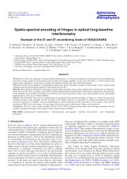
Figure 1.1: (Top) The primary rotation period of the known NEA (filled) and MBA(open) binaries as a function of the pericenter of the binary’s orbit. (Bottom) The componentseparations of the same binaries as a function of pericenter. In both panels, eachpoint represents one binary, with the size of the point indicating the size of the primary.10

Table 1.2.Binary MBA properties.Binary a e D pri P pri a D sec P orb Disc. ref(AU) (km) (h) km (km) (d)(4674) Pauling 1.86 0.07 8 250 2.5 AO [1](1509) Esclangona 1.87 0.03 12 2.64 140 4 AO [2,3](9069) Hovland 1.91 0.11 3 4.22 0.9 L [4](5905) Johnson 1.91 0.07 3.6 3.783 1.44 1.16 L [4,5](76818) 2000 RG 79 1.93 0.10 3.6 3.166 1.1 0.59 L [36](1089) Tama 2.21 0.13 13 16.44 20 (9) 0.68 L [6](3749) Balam 2.24 0.11 7 350 1.5 100 AO [7,8](3703) Volkonskaya 2.33 0.13 3 3.23 1.2 1 L [36](854) Frostia 2.36 0.17 1.57 L [9](3782) Celle 2.41 0.09 6.1 3.84 36.57 2.6 1.52 L [10,11](11264) Claudiomaccone 2.58 0.23 4 3.18 1.2 0.63 L [36](1313) Berna 2.65 0.20 25.46 1.061 L [12](45) Eugenia 2.72 0.08 215 5.70 1190 13 4.69 AO [8,13](4492) Debussy 2.76 0.17 26.59 1.11 L [14](22899) 1999 TO 14 2.84 0.08 4.5 170 1.5 HST [15](17246) 2000 GL 74 2.84 0.02 4.5 230 2 HST [16](243) Ida 2.86 0.05 31 4.63 108 1.4 1.54 SC [8,17](22) Kalliope 2.91 0.10 181 4.14 1020 38 3.58 AO [18,19,20](283) Emma 3.04 0.15 148 6.88 600 12 3.36 AO [21,22,23](130) Elektra 3.12 0.21 182 5.22 1250 4 3.9 AO [21,24,25](379) Huenna 3.13 0.19 92 7.02 3400 (7) 81 AO [23,26,27](90) Antiope 3.16 0.16 85 16.50 170 85 0.69 AO [8,28](762) Pulcova 3.16 0.09 137 5.84 810 20 4.0 AO [8,29](121) Hermione 3.43 0.14 209 5.55 775 13 2.57 AO [30,31,32,33](107) Camilla 3.47 0.08 223 4.84 1240 9 3.71 HST [8,34](87) Sylvia 3.49 0.07 261 5.18 1360 18 3.65 AO [8,35,37](87) Sylvia 3.49 0.07 261 5.18 710 7 1.38 AO [37]Note. — Orbital and physical properties for well-observed or suspected MBA binaries. The discovery techniquesare (L) lightcurve, (AO) adaptive optics, (T) ground-based telescope, and (SC) for spacecraft. References:[1] Merline et al. (2004); [2] Merline et al. (2003b); [3] Warner (2004); [4] Warner et al. (2005a); [5] Warneret al. (2005b); [6] Behrend et al. (2004b); [7] Merline et al. (2002a); [8] Merline et al. (2002c); [9] Behrend et al.(2004a); [10] Ryan et al. (2003); [11] Ryan et al. (2004); [12] Behrend et al. (2004c); [13] Merline et al. (1999);[14] Behrend (2004); [15] Merline et al. (2003d); [16] Tamblyn et al. (2004); [17] Belton & Carlson (1994); [18]Merline et al. (2001); [19] Margot & Brown (2001); [20] Marchis et al. (2003); [21] Marchis et al. (2005a); [22]Merline et al. (2003c); [23] Stanzel (1978); [24] Merline et al. (2003e); [25] Magnusson (1990); [26] Margot(2003); [27] Harris et al. (1992); [28] Merline et al. (2000b); [29] Merline et al. (2000a); [30] Merline et al.(2002b); [31] Merline et al. (2003a); [32] Marchis et al. (2004a); [33] Marchis et al. (2004b); [34] Storrs et al.(2001); [35] Brown et al. (2001); [36] Pravec et al. (2006); [37] Marchis et al. (2005b).11

1.2.1 CaptureIn this scenario two asteroids become mutually bound during a close encounter. Requiredduring this encounter are relative speeds that are below their mutual escape speeds. For thesmall bodies of the NEA population the escape speeds are generally on the order of m s −1 ,while encounter speeds are on the order of km s −1 . As well the time between encountersis longer than the dynamical lifetime for the bodies. Capture is similarly unlikely in theMain Belt, eliminating the possibility of a captured system in this population migratinginto the NEA population. As well, captured binaries would be expected to be only looselybound, and would have a very short lifetime in the NEA population before a planetaryencounter disrupted the system. The capture scenario is best suited to very wide binariesobserved in the Kuiper Belt.1.2.2 CollisionsBoth catastrophic and subcatastrophic impacts can create a debris field capable of reaccumulatingsecondaries around a massive central remnant, or having debris leaving thesystem become bound to each other. Hypothesized by van Flandern et al. (1979) and Weidenschillinget al. (1989) as a possible mechanism for binary formation, it needs to overcomethe fundamental problem that debris leaving the surface of a spherically-symmetricasteroid will have its bound orbit pass through the surface of the asteroid. Weidenschillinget al. (1989) posited that dense debris fields with accumulated secondaries whose final orbitis determined by their mean angular momentum is a possible solution.After the discovery of Ida’s satellite, Dactyl, numerical simulations of an expandingdebris field resulting from a collision and disruption of an asteroid found that many differentkinds binary systems were created (Durda 1996). Using assumed ejecta patternsand mass distributions, numerous binary configurations were observed, with a wide range12

of size ratios, including contact-binary formations.In the course of modeling asteroid family formation via reaccumulation of debris followinga catastrophic impact, Michel et al. (2001, 2004) found many companions of thelargest remnant. The works were focused on, and matched, many dynamical and physicalproperties of some asteroid families, but no comprehensive analysis of any binaries wascompleted.Durda et al. (2004) simulated large-scale (100 km diameter target body) catastrophiccollisions of asteroids to determine the efficiency of forming binaries via collision. Similarto Michel et al. (2001, 2004) these simulations used a smoothed particle hydrodynamics(SPH) code to model the collision and an N-body code to simulate the post-collisionevolution and re-accumulation of the fragments. The collisions were efficient at creatingbound systems out of the re-accumulated debris and many of the binaries producedare qualitatively similar to those observed in the Main Belt. Two main types of outcomesfrom these simulations were observed and classified as SMATS (SMAshed TargetSatellites) and EEBs (Escaping Ejecta Binaries). The SMATS consist of re-accumulatedfragments orbiting the largest remnant from the collision, whereas the EEBs are small andusually similar-sized fragments that have escaped from the largest remnant and becomebound to each other.Of the observed MBA binaries discovered via high-resolution imaging most are similarto SMATS, with primaries significantly larger than the secondaries. Some binarieswith small, nearly equal-sized components and large separations are suspected EEBs (see(4674) Pauling, (1509) Esclangona, (22899) 199 TO 14 , and (17246) GL 74 in Table 1.2).In the NEA population the collisional lifetimes are significantly longer than the veryshort dynamical lifetimes (∼10 Myr as determined through numerical simulations), makingcollisions an unlikely local source of binaries. The binaries observed in collisionsimulations typically have larger separations than is observed with NEA binaries. How-13

ever, understanding the mechanism is important as collisionally formed binaries in theMain Belt may migrate to the NEA population.1.2.3 Rotational disruptionRotational disruption has been credited with a large role in binary formation among NEAsdue to some of the prominent similar properties shared by these binaries (Merline et al.2002c; Margot et al. 2002). Rapidly-rotating primaries, very near the theoretical breakuplimit for strengthless bodies, have been a signature of binary NEAs and have recentlybeen seen among small MBAs. The fastest-rotating NEAs have periods no shorter than ∼2 h, and the primaries of the observed binaries nearly all have periods below 3 h. Thus aformation related to rotational disruption when an asteroid is made to spin faster than thecritical limit has been favored for this population.Tidal disruptionTidal disruption of a rubble pile has been invoked to explain the disruption of CometD/Shoemaker–Levy 9 (SL9) and has also been applied to asteroid studies. SL9 disruptedwhen the comet passed within ∼ 1.36 R J of Jupiter on 1992 July 7. The comet was tornapart and ∼ 21 fragments or reaccumulated clumps were later observed. N-body studieshave since matched many of the comet’s basic post-disruption features (train length, positionangle and morphology) using a strengthless rubble pile model (Solem 1994; Asphaug& Benz 1996; Walsh et al. 2003).Solem & Hills (1996) used similar N-body techniques to simulate the change in elongation(ratio of long axis to short axis length) of an asteroid due to a planetary closeapproach. Citing 1620 Geographos as an extreme case with an elongation of 2.7, encounterswith Earth between close approach distance q = 1.02 and 2.03 Earth radii (R ⊕ ) weresampled with a range of v ∞ (the speed at infinity of a hyperbolic encounter) between ∼14

15 and 25 km s −1 . The models represented the progenitors with 135 particles, and somesimulations produced outcomes more elongated than Geographos, providing a potentialmeans of creating very elongated solar system bodies.Bottke & Melosh (1996a) simulated splitting of contact binaries to explain doubletcraters on Earth, Venus and Mars. In this model a binary asteroid is formed during a closeencounter with a planet, and the binary’s separation grows through subsequent encounters.Eventually the binary hits a planet, making a doublet crater. This scenario depends on aconstant refreshing of the NEA binary population via tidal disruptions, and predicts that∼ 15% of NEAs may be binaries at any given time.Simulations of NEA tidal disruption by Richardson et al. (1998) covered a large parameterspace of elongated rotating bodies (constructed with 247 particles) passing Earthat various q and v ∞ . The study was designed to quantify disruption and mass loss fortidal encounters, but noted binary formation as an observed outcome and suggested thattidal disruption could explain up to ∼ 15% of the NEAs being binaries. The simulationssparsely covered the parameters of q, v ∞ , progenitor elongation, progenitor spin rate andlong axis alignment. Basic trends in disruption were observed, with increasing disruptionfor closer approaches, slower approach speeds, and faster prograde rotation rates. Moresubtle results were seen as a function of body elongation and long axis alignment at closeapproach.Functionally tidal disruption is an impulsive event that both elongates and torques abody. A spherical body will be elongated and then spun-up during a passage by a planet,whereas a previously elongated body may be reshaped or just spun-up more dramaticallydepending on the long-axis alignment during close approach. In the closest and mostcatastrophic encounters a strengthless body is pulled into a long string of particles, similarto the SL9 event, and numerous clumps form along the string. A less dramatic event willsimply involve a body appearing to have been spun-up to the point that some mass escapes15

off the equator or off one end of a prolate body.Bottke et al. (1999) compared the shape of 1620 Geographos, obtained from delay–Doppler measurements, to that of a tidal encounter outcome. The well-defined shape ofGeographos matched many features of the simulation output, including the cusped ends,an opposed convex side, and a nearly concave side with a large hump. This study wassimilar in approach to Solem & Hills (1996), but matched the high-quality images withhigh-resolution (∼ 500-particle) simulations.Thermal SpinupAn alternative mechanism for rotational disruption is the YORP thermal effect (see Bottkeet al. 2006 for a review). This effect, related to the Yarkovsky effect, relies on re-emissionof absorbed solar radiation to provide a very small thermal thrust. This thrust, over longtimescales, provides a torque which can alter the asteroid’s obliquity and spin rate. Thiseffect depends heavily on the size of the asteroid, and is expected to be quite powerfulfor sub-kilometer bodies (with spin rate doubling timescales on the order of 0.5 Myr)and ineffective for diameters larger than 40 km. Suggested as possibly responsible forthe excess in fast and slow rotators among small asteroids, YORP has been shown in onedramatic case to re-orient spin axes. Vokrouhlický et al. (2003) demonstrated that thecombination of thermal torques from YORP and spin-orbit resonances created a collectionof similar spin periods and obliquities among Koronis family members, matchingobservations perfectly.Despite these detailed studies of the YORP effect, binary creation from thermal spinuphas yet to be studied in detail. Any detailed study relies on various assumptions aboutan asteroid’s shape and thermal properties, as well as the dynamics of a body that hasreached and passed its critical spin frequency. The discovery of binaries in the Main Belt,resembling those in the NEA population, strongly suggest that a thermal force is helping16

to create or change binaries within both populations.1.3 Shape and Spin Distributions for NEAs and MBAsThe shape and spin distributions for NEAs and MBAs tells a significant story about eachpopulation. The first theories that asteroids may be strengthless, or even rubble piles,came from analysis of the spin periods derived from lightcurves (Burns 1975; Harris1996). As well, it was concerted campaigns to collect lightcurves of NEAs which starteddiscovering binaries (Pravec & Hahn 1997). The spin and shape of asteroids has alsoproven to be important parameters in determining the outcome of tidal disruption simulations(Richardson et al. 1998), which is why they are of interest in this work. From themeasured lightcurve, an asteroid’s rotational period can be estimated assuming that anynormal elongation will produce a double-peaked periodic curve. The amplitude of thiscurve is related to the axis ratio of the asteroid via equation 1.3.1.3.1 Existing lightcurve dataThe repository for published asteroid lightcurves contains the best parameters for all observedsmall bodies (Harris et al. 2005a). A rating system is employed to differentiatebetween data of different quality,0 Result later proven incorrect. This appears only on records of individual observations.1 Result based on fragmentary lightcurve(s), may be completely wrong.2 Result based on less than full coverage, so that the period may be wrong by 30 percentor so. Also, a quality of 2 is used to note results where an ambiguity exists as to thenumber of extrema per cycle or the number of elapsed cycles between lightcurves.Hence the result may be wrong by an integer ratio.17

3 Denotes a secure result with no ambiguity and full lightcurve coverage.4 In addition to full coverage, denotes that a pole position is reported.Significant temporal coverage of an asteroid’s rotation period is required to estimate theperiod with any certainty, and, as the rating system implies, even extensive observationscan still leave certain parameters in doubt. When compiling statistics about differentpopulation’s shape and spin from lightcurve data, the rating system is an important toolin understanding previously published data.Currently in the lightcurve repository there are 60 Main Belt objects with a diameter< 5 km for which a minimum quality (Q) of 2 is listed. There are 225 such observationsfor bodies with diameter D < 10 km and 480 with D < 20 km. From this list none ofthe small (D < 5 km) MBAs are binary asteroids, and there are 289 NEAs listed in therepository, among which 15 are binaries.1.3.2 Recent studiesBinzel et al. (1992) presented the results of a dedicated survey of MBAs smaller thanD < 5 km. The survey covered 32 objects and presented 30 periods and 32 amplitudesfrom lightcurves. Overall the results suggested that the sample had a rotational frequencyfaster than the population of larger MBAs. This was the first survey of this kind, and nosimilar dedicated survey of small MBAs (SMBAs) lightcurves has followed.Pravec et al. (2002) summarizes asteroid rotations highlighting how spin rate varieswith size. Using a running box statistical method they report that the geometric mean spinperiod for D > 40 km is ∼13 h, and decreases to ∼ 6 h for D ∼ 10 km. The distributionfor asteroids with D > 40 km, is fit well with a maxwellian distribution, whereas for 0.15< D < 10 km is not. This group of smaller asteroids, which includes NEAs, has strongpopulations of slow (∼30 h) and fast (∼3.5 h) rotators, with an apparent maximum spin18

arrier around 2.2 h. The excess of both fast and slow rotators in the NEA populationhas been suggested as a possible manifestation of the YORP thermal effect (Pravec et al.2002; Bottke et al. 2006).Scheeres et al. (2004) analyzed the nature of rotation changes due to the close encounterswith planets that NEAs undergo. This study quantified the overall increase in spinrate that a population would gain through these encounters by modeling a steady-statesystem where Main Belt asteroids become NEAs, have encounters over their lifetime andare then replaced by new MBAs. This Monte Carlo simulation used the rotation ratesfrom Donnison & Wiper (1999) derived from collisional experiments as the initial MBArotation rate distribution. This distribution was then compared to the steady-state distributionof NEAs that evolved over time through planetary encounters. Overall a slightspin-up of rotation rates was noted, and the maximum spin achieved from an encounterwas near the classical critical breakup limit of 2 h. This study confirmed that the NEApopulation will have a spin-rate distribution different from its parent bodies in the MainBelt.1.3.3 Motivation for work on small MBAsDue to observational constraints it is significantly more difficult to obtain lightcurvesfor kilometer-sized MBAs than for the closer NEAs. Thus direct comparisons betweensimilarly sized NEAs and MBAs is nearly impossible, as the number of lightcurves forsmall MBAs is currently inadequate. Each population has differing dynamical environments,with short lifetimes and frequent planetary encounters for NEAs and much shortercollisional than dynamical lifetimes in the Main Belt. They also have differing thermalenvironments, with the more distant MBAs less affected by the Yarkovsky or YORP thermaleffects. Because of the sometimes powerful effects these phenomena may have onthe shape and spin of small asteroids, detailed studies of lightcurves are potentially diag-19

nostic.Recent results have demonstrated that the effectiveness of tidal disruption at binaryformation has a strong dependence on the shape and spin of a strengthless asteroid encounteringa planet (Walsh & Richardson 2006, Chapter 2). In order to place tidal disruptionsimulations into a larger model of MBA-NEA binary formation and evolution itis necessary to understand the properties of small MBAs (D < 5 km, SMBAs). The NEApopulation is roughly a steady-state population with asteroids being removed via encounters/collisionswith planets and the Sun, and being refilled by eccentricity-pumping resonancesin the Main Belt (Bottke et al. 2002). Though there are many NEA lightcurvesthat are well characterized, these will represent the shape and spin of bodies which mayhave already had their spin state altered due to close encounters with planets (Scheereset al. 2004). The lightcurves of SMBAs however, should provide the spin and shapedistribution of asteroids which first encounter planets after entering an NEA orbit.Photometric lightcurves have successfully discovered ∼ 17 binary asteroids in theNEA population, and ∼ 13 in the Main Belt (Pravec et al. 2006). Up until 2004 allMBA binaries had been discovered via high-resolution ground- or space-based imaging,whereas most NEA binaries were discovered via lightcurve observations.1.4 Steady-State Models of the NEA PopulationThe NEAs are essentially a transient population, with short lifetimes on the order of10 Myr, but roughly constant overall numbers due to migration of asteroids from theMain Belt (Bottke et al. 2002). Comparison of binary formation simulations with theobserved population requires the properties of the simulated binaries, as well as inclusionof the dynamic lifetimes of the bodies and any known evolutionary effects. The modeledpopulation changes over time, as binaries are created and evolve, and are replaced by20

single bodies at the end of their lifetime. The steady-state population that evolves can thenbe compared with the observed population, revealing the importance of tidal disruptionin forming binary NEAs.1.4.1 Near-Earth asteroid population dynamicsThe NEA population consists of those asteroids with perihelion distances q ≤ 1.3 AUand aphelion distances Q ≥ 0.983 AU (Rabinowitz 1994; Bottke et al. 2002). Earth andMoon cratering records suggest an impact flux that has remained roughly constant overthe past 3 Gyr, implying that the NEA population has not varied drastically in numbersover that time (Grieve & Shoemaker 1994). Therefore bodies being removed from theNEA population (via collision with a planet or the Sun, or by ejection from the innersolar system) must be replaced to keep the population constant.Prior to the first studies indicating that resonances can cause significant increases inan asteroid’s eccentricities, it was thought that many NEAs were extinct cometary nuclei.However, eccentricity-boosting resonances provide a means for MBAs to migrateonto planet-crossing orbits and eventually into near-Earth space (Wetherill 1979; Wisdom1983). It was thought that frequent catastrophic collisions or large impacts withejected debris would cause material to be injected into two powerful resonances in theinner Main Belt: the ν 6 secular resonance with Saturn and the 3:1 mean motion resonance(MMR) with Jupiter. Once material is injected into these resonances, it will haveits eccentricity pumped and enter an Earth-crossing orbit on a short timescale. MonteCarlo simulations of the asteroid transport into these two resonances and subsequentlyinto near-Earth space traced the evolution of asteroids into NEAs, but did not account forthe inherently chaotic environment later revealed with the first numerical investigations(Wetherill 1988; Rabinowitz 1997a,b; Gladman et al. 2000).A series of works has suggested that Mars-crossing asteroids can be considered as21

another intermediate source of NEAs in addition to the two previously cited resonances.Migliorini et al. (1998) asserted that the Mars-crossers that are not NEAs (q > 1.3 AU)have histories inconsistent with an origin from the 3:1 MMR or the ν 6 secular resonance.It was also shown that a series of weak mean-motion resonances with Jupiter or Mars,along with three-body mean-motion resonances with Jupiter and Saturn, can increase anasteroid’s eccentricities until it is on a Mars-crossing orbit (Morbidelli & Nesvorny 1999).From a Mars-crossing orbit an asteroid can evolve into an NEA on timescales of only tensof millions of years (Migliorini et al. 1998; Michel et al. 2000).Bottke et al. (2002) modeled the transport of asteroids from 5 different source populationsin the Main Belt, matching their resultant NEA orbits to a debiased NEO populationfit to Spacewatch data. This work found that the majority (∼61%) of the NEA populationmigrates from the inner Main Belt (a < 2.5 AU), with the central Main Belt (2.5 < a < 2.8AU) contributing ∼24%. This established the NEA population as a steady-state populationconsisting mostly of inner Main Belt asteroids that migrated via one of three mainsources; the two inner Main Belt resonances or from intermediate Mars-crossers.1.5 Background1.5.1 Tidal disruptionThe model for a tidal disruption of a small, non-rotating, liquid satellite in orbit arounda massive body was initially provided by Roche (1847) (see Chandrasekhar 1969). Thiswork solved for the orbital radius inside of which the small body on a circular orbit cannotmaintain an equilibrium figure under the strain of tidal forces. This limit is( ) 1/3 ( ) 1/3 Mpρpr Roche = 1.52 = 2.46R p (1.4)ρ s ρ swhere M p , R p and ρ p are the mass, radius and density of the planet, and ρ s is the density22

of the satellite in question. For an asteroid of density 2.0 g cm −3 , the Roche limit wouldbe ∼ 3.45 R ⊕ about Earth.In an attempt to extend this limit to solid bodies, Jeffreys (1947) considered internalstrength. He applied his solution to asteroids breaking up around the Earth and Jupiter, aswell as the formation of the rings of Saturn from objects with the consistency of ice. Hiscalculations estimated high internal strengths, and therefore determined that tidal forces,which increase with size, could only be effective on objects with a diameter roughly> 200 km. After the discovery of Comet Ikeya-Seki in 1965, Opik (1966) consideredmodels of tidal disruption for the sun grazing family of comets, and included self-gravity.Opik (1966) suggested that Ikeya-Seki may have had a rubble-pile structure and evenmade qualitative arguments about the effect that the direction of the axis of rotation couldhave on a tidal disruption.In their study of self-gravitating, non-rotating viscous bodies during parabolic encounterswith planets Sridhar & Tremaine (1992) showed that small bodies can shed mass ordisrupt entirely. They determined a pericenter distance inside of which disruption or massloss would occurr disrupt < 1.69R p(ρpρ s) 1/3(1.5)which is smaller than the classical Roche limit. For non-viscous bodies that are heldtogether by self-gravity they determined that the bodies would behave approximately likethe viscous fluid.Richardson et al. (1998) used rubble pile models to simulate tidal disruption of Earth–crossing asteroids. These simulations explored a parameter space which included theasteroid’s hyperbolic encounter (periapse q and encounter velocity with Earth v ∞ ), spinperiod P and shape–orientation conditions. The outcomes were parametrized by the massstripped off during the disruption, or the distortion of the body.23

1.5.2 Rubble pilesThe evidence for non-monolithic solar system objects is of considerable importance fortidal disruption scenarios, as internal strength can frustrate disruptions. Evidence for asignificant population of strengthless bodies dates to work by Burns (1975), where theyexamined the spin angular momentum of 70 asteroids and compared the centrifugal accelerationsto the bodies’ self-gravity. The critical spin period scales with ρ −1/2 thusdemanding a shorter period for denser objects. For all asteroids in the sample with anassumed density of 3 g cm −3 the gravitational force exceeded that of the centrifugal thuspermitting these objects to be held together strictly by self-gravity. The lack of objectswith a very rapid rotation rate suggests that internal structures do not allow rapid rotation.A huge database of asteroid light curves (688) was used by Harris (1996) to evaluatepossible rubble pile structure of asteroids. The lack of objects with very fast spin periodagain suggests an overall trend of asteroids of very low internal strength. The cutoff inrotation rate is at the critical spin rate for a density of ∼ 2.7g cm −3 , a density thought tobe typical for asteroids, suggesting that no faster rotation rates are observed because ingeneral these asteroids have no internal strength.In a review of the studies on strengthless bodies, Richardson et al. (2002) establishedterminology stating that a rubble pile is moderately porous, strengthless body with constituentsbound only by their own self-gravity. This differs from a shattered, or fracturedbody, which may have no strength, but also low porosity. A numerical model of a “perfect”rubble pile, will by necessity have moderate porosity (at least ∼30%), and currentlyno techniques incorporate strength. Citing evidence from cometary breakup, crater chainson planetary moons, doublet craters, asteroids spin rates, low asteroid densities, giantcraters on asteroids, linear grooves on surfaces and binary asteroids, this work provideda strong case for the theory that many or most bodies between the sizes of ∼100 m and24

∼100 km are rubble piles.1.6 This DissertationThis dissertation was designed to investigate the role of tidal disruption in the formationof binary NEAs. At the heart of this work is the attempt to answer the following threequestions,1. What are the properties of tidal-disruption-formed binaries and how do they compareto the observed NEA binaries?2. What is the spin and shape distribution for small MBAs, how does it compare toNEAs and large MBAs?3. What is the overall steady-state binary fraction for NEAs caused by tidal disruption?We present theoretical and observational studies to address all three questions in thefollowing chapters. First, in Chapter 2, we describe our models of the tidal disruptionof strengthless “rubble pile” asteroids, using N-body simulations. Results from manysimulations covering a large parameter space are presented, with characterization of thebinaries formed.In Chapter 3 an observing campaign designed to study the shape and spin of smallMBAs is presented. Observations of 28 asteroids are combined with previously publishedlightcurves to determine the shape and spin distribution for small MBAs.The results from the observations in Chapter 3 are used along with the simulation resultsin Chapter 2, to create a steady-state model of the binary NEA population presentedin Chapter 4. This model tracks binary NEAs as they are formed, evolve and eventuallyreplaced when they reach the end of their lifetime.In Chapter 5 we summarize the main results and present conclusions.25

Chapter 2Formation of Binary Asteroids via TidalDisruption of Rubble PilesWalsh & Richardson, 2006, Formation of Binary Asteroids via Tidal Disruption of Rubble Piles,Icarus 180, 201–2162.1 OverviewIn this chapter we adopt numerical techniques similar to those of previous N-body rubblepile simulations, and cover parameters previously shown to produce catastrophic tidalencounters, but in much greater detail. This study is unique in the large number of simulationsperformed and detailed investigation into the physical and orbital attributes of theresulting binaries. In Section 2.2 the details of the simulations and analysis are explained,and the results are discussed in Section 2.3. Conclusions and future work are presentedin Section 2.4.26

2.2 Method2.2.1 SimulationsAll simulations were done using pkdgrav, a parallelized tree code designed for efficientN-body gravitational and collisional simulations (Richardson et al. 2000; Leinhardt et al.2000; Stadel 2001; Leinhardt & Richardson 2002; Richardson et al. 2005). The simulationsused a timestep of 10 −5 yr/2π, (about 50 seconds, or ∼ 2% of the dynamical timefor the particles) and all simulations were initially run for 10,000 timesteps (∼ 5.8 days).Simulations that produced binaries or systems of bound bodies were run an additional20,000 timesteps to reach a total of 30,000 timesteps (∼ 17.4 days). The collisions ofindividual particles were governed by coefficients of restitution, both normal (ε n ) andtangential (ε t ), which determine how much energy is dissipated during collisions. Thenormal coefficient of restitution, ε n , was fixed at 0.8 in these simulations, similar to previousstudies, and ε t was fixed at 1.0 (no surface friction). Previous work has shown thatε n has little effect on the outcome of a tidal disruption so long as ε n < 1.0 (Richardsonet al. 1998).2.2.2 ProgenitorsThe rubble pile models used in these simulations consist of identical rigid spheres boundto one another by gravity alone. There were five separate progenitors used in the simulations,each with different elongations: 1.0, 1.25, 1.5, 1.75, and 2.0 (here elongationis defined as e = a/c with a, b and c representing the long, intermediate and short axislength of a tri-axial ellipsoid; in our simulations, b was set to ∼ c). The bodies were allconstructed using particles with an internal density of 3.4 g cm −3 , but the bulk densityof the body would vary depending on its packing efficiency, which was usually around27

∼ 60%, making a bulk density of ∼ 2.0 g cm −3 . Each progenitor consisted of approximately1,000 particles; the exact number varied between 991 and 1021 depending on thefinal overall shape 1 . Recent work by Richardson et al. (2005) shows that the resolutionof a rubble pile simulation can have an effect on the outcome: as resolution increases, thegranular behavior becomes more fluid-like, aiding disruption. To justify our use of 1000particles, we assume the smallest building block for rubble piles in the inner solar systemis ∼150 m, based on SPH collision studies and the observed spin rate cutoff of km-sizedasteroids (Benz & Asphaug 1999; Pravec et al. 2002). With 150 m particles, a sphericalclose-packed rubble pile with 1000 particles is ∼ 3.3 km in diameter. This diameter isnearly as large as the largest observed NEA binary primary, but also has enough resolutionto model ejected fragments which may remain bound to each other, and to allowaccurate measurement of size ratios.The progenitors were given one of four rotation rates: 3, 4, 6, or 12 h periods. Largeasteroid (D > 40 km) spin rates have been shown to follow a Maxwellian distribution,but small asteroids (D < 10 km) have an excess of fast and slow rotators (Pravec et al.2002). Studies have attempted to fit the population of small asteroids with 3 differentMaxwellians, with a combination of fast, moderate, and slow rotation rates of ∼ 6.4, 11.3,and 27.5 h (Donnison & Wiper 1999). However, with the large proportion of fast-rotatingNEAs (possibly as high as 50%) observed to be primaries of binary systems, they mayhave already experienced a tidal disruption and had their spin state altered (Margot et al.2002; Scheeres et al. 2004). Our selections were made to sample fast rotators (3, 4 h), aswell as some moderate ones (6, 12 h). No spin periods longer than 12 h were simulated1 The packing algorithm uses hexagonal closest packing, which depends on a certain level of symmetryto construct bodies out of a finite number of perfect spheres. This results in variation in the number ofparticles for various shapes. Similarly, due to boundary algorithms and the finite size of the building blocks,the bulk density can vary slightly.28

Figure 2.1: Progenitor initial parameters of the reciprocal of elongation (c/a) and normalizedangular spin frequency (ω/ √ 2πGρ) are plotted as points. (solid line) This iscompared with the limiting curve for a cohesionless granular proloid with friction angleφ = 40 ◦ (Holsapple 2001; Richardson et al. 2005). (dashed line) The solutions for Jacobiand Maclaurin sequences representing theoretical axis ratios for rotating fluids.due to the small contribution rotation actually makes to tidal disruption at slower spins(Richardson et al. 1998).The 3 h spin rate simulations were only carried out for progenitors with an elongationof 1.0 and 1.25. Comparison to Richardson et al. (2005), as well as separate tests, indicatethat bodies with elongation of 1.5 or greater would be unstable at a 3 h spin rate, thus29

shedding mass and distorting prior to encountering the tidal forces of Earth (Fig. 2.1).The subset of results for 3 h will be presented independent of the bulk of the studies.The progenitors used in this work are all below the limit for cohesionless granularproloids with friction angle φ = 40 ◦ (Holsapple 2001). This limit, verified by Richardsonet al. (2005) as a rotational stability limit for numerical models of rubble piles, differsfrom the Maclaurin/Jacobi limits for fluid bodies (essentially a sequence of allowed equilibriumshapes). The Maclaurin/Jacobi sequence can be derived analytically and providesa useful fiducial for comparing less idealized models. For example Guibout & Scheeres(2003) determined that when a body is spinning beyond the Jacobi limit, the flow of materialon the surface of the body is towards the equator, whereas below the limit, the flowis towards the poles.2.2.3 Tidal encounters and initial conditionsThe hyperbolic encounters asteroids have with planets can be described by the close approachdistance q and the relative speed at infinity v ∞ . When v ∞ ≫ v esc (where v esc =√2GM/R), close approach is distributed with likelihood increasing as the square of thedistance. This means that an asteroid is four times more likely to encounter Earth at 4 R ♁than at 2 R ♁ . The v ∞ of these encounters depends on the bodies’ pre-encounter orbits.A distribution of expected encounter statistics was taken from a series of N-body simulationsof NEA migration from major source regions in the Main Belt (3:1 mean-motionresonance with Jupiter, ν 6 secular resonance, Mars crossers; Bottke et al. 2002, Bottke2004 personal communication; the distribution is similar to the impact speed distributionof Bottke et al. 1994). This was used to determine the expected v ∞ for the hyperbolicencounters with Earth (Fig. 2.2). Simulated parameters were selected to cover the mostfrequently occurring encounters and those previously shown to create very disruptive encounterslikely to form binaries, all sampled at a frequency to balance detail with compu-30

Figure 2.2: The distribution of v ∞ for close hyperbolic encounters with Earth, with v ∞in km s −1 and the y-axis indicating the normalized probability for each v ∞ bin (Bottke2004, personal communication).tational expediency: q=1.2, 1.4, 1.6, 1.8, 2.0, 2.2, 2.4, 2.6, 2.8, 3.0, 3.5, 4.0 and 4.5 R ♁and v ∞ = 8, 12, 16, 20, and 24 km s −1 .Richardson et al. (1998) determined that the orientation of a non-spherical body canhave a significant effect on the outcome of a tidal disruption. Specifically when the leadinglong axis of a body is rotating towards or away the planet, disruption is enhanced orsuppressed respectively. Near perigee the equipotential surface of the body is stretched in31

Figure 2.3: Snapshots of a tidal disruption simulation that led to the formation of a binaryasteroid. The frames span about 72 h.the direction of Earth, and particles may rearrange to fill that shape (see Fig. 2.3 for a representativedisruption). So if the long axis is rotating away from the planet, the rotation ofthe body opposes the movement of the particles. Instead of parameterizing the specificsof body axis alignment, a compromise was made: for each set of encounter (q and v ∞ )and body (elongation and spin rate) parameters, the simulation was run 100 times, eachtime randomizing the orientation of the body’s spin axis. Thus, given that the hyperbolicencounters were always in the same plane, some bodies were spinning prograde and someretrograde with respect to the encounter with Earth, depending on the randomization outcome.The long axis position at perigee was also random. This means that each set ofparameters has a distribution of possible outcomes rather than one unique solution.2.2.4 AnalysisIdentification of orbiting systems was done using the companion code (Leinhardt &Richardson 2005). This code is optimized for extremely fast searches over all simulations,identifying and analyzing those with bound systems. First, each simulation wassearched for re-accumulated clumps of particles (Leinhardt et al. 2000). Once the clumpswere identified, those consisting of more than three particles were fed into companion tosearch for systems. Any bound clumps were then analyzed to obtain important physicalparameters, such as spin vector, elongation, mass, radius and position/velocity vectors.The code companion sorts binaries according to identification of the primary andsecondary clumps. In a situation where a specific clump has multiple secondaries, it will32

Total Binaries T-PROS T-EEBs Prolate Oblate S-class B-class M-class4939 4556 383 4692 246 226 2299 24143 h spin periods; 1.0 and 1.25 elongations only798 702 96 740 58 59 357 382Table 2.1: Cumulative statistics from all 110,500 simulations. Total binaries is simplya count of all systems observed in the simulations. T-PROS and T-EEBs represent thetotal binaries split into dynamical groups (see Section 2.3.2). Prolate and Oblate columnsseparate the binaries according the shape of the primary body (see Section 2.3.1). Thebinaries are also separated according to the class of disruption in which they were formed,S-class being the most disruptive, followed by B-Class and M-Class (see Section 2.3.3).be listed once for each. Thus a triple, or larger, system may result in the same primarybeing counted multiple times in the statistics presented. The situation of an hierarchicalsystem, where a secondary body itself has an orbiting clump, will result in that body beingcounted as both a secondary and a primary.2.3 Results and Discussion2.3.1 Bulk resultsThe bulk results covered 1,105 sets of parameters, which encompasses 110,500 total simulations.From these simulations a total of 5,737 bound systems were found after 30,000timesteps (see Table 2.1 for a summary of bulk statistics). Of all the binaries, 798 wereformed in the subset of 3 h, low-elongation simulations (to be referred to as the 3 h subset,and not included in plots or tables unless specifically mentioned; see Section 2.2.2 andSection 2.3.4).Figure 2.4 shows the relative contributions each parameter made to binary production.The trends are consistent with the findings of Richardson et al. (1998). The lower the v ∞ ,the more disruptive the outcome, and hence more binary formation results. Likewisebinary production falls off very smoothly as q increases. The spin period distribution33

Figure 2.4: Normalized probability of binaries formed versus (a) q, (b) v ∞ , (c) initial spinrate and, (d) initial elongation.shows the dramatic increase in production at high spin rates, as bodies with 4 h periodswere nearly 60% more likely to create a system than those with a 6 h period. Similarly,elongated bodies were significantly more efficient at producing binaries, with elongationsof 2.0 making nearly 3 times the number of binaries as elongations of 1.0 or 1.25.Figure 2.5 displays the number of binaries formed as a function of the mass of thelargest remnant divided by the mass of the progenitor, basically a measure of how disrup-34

tive the encounter was. This measure was used by Richardson et al. (1998) to delineate 3classes of tidally disruptive encounters:1. S-class disruption: Named for an SL9-type disruption where the largest remnant has nomore than 50% of the progenitor’s mass. This class of disruptions is the most dramatic,as the progenitor is stretched into a long trail of particles before numerous clumps takeshape. Binaries can be created if two clumps form close enough to become bound, or if aclump has accreted multiple fragments.2. B-class disruption: A rotational breakup where the largest remnant contains between50% and 90% of the mass of the progenitor. A B-class breakup involves a similar situationas the S-class, but less extreme, allowing a central large clump to form from the distortedand stretched progenitor.3. M-class disruption: A mild breakup with less than 10% of the mass of the progenitorlost during the disruption. As the body is spun up, it is stretched along its long axis, particlesslide to the equator of the body, and many are launched off the main body. Unlike themore disruptive breakups where a long chain of particles separates into separate clumps,the M-class encounters appear more like a body that starts spinning too fast (beyond theJacobi and related cohesionless granular proloid limits), distorts, and then sheds massfrom its equator.Binary production peaks for encounters classified as M-class, with the largest remnantcontaining 90% to 95% of the mass of the progenitor. With a large percentage of the masscontained in the largest remnant, the binaries formed are limited to small size ratios. B-class and M-class outcomes account for nearly equal amounts of the binaries created andabout 95% of the total created.35

Figure 2.5: Normalized probability of binaries formed versus the mass of the largestremnant divided by the mass of the progenitor. The vertical lines separate the disruptionsinto defined classes, with S-class being most disruptive, followed by B-class and M-class(Richardson et al. 1998). The percentages represent the total number of binaries in eachclass36

Orbital propertiesThe eccentricity distribution in the simulations is dominated by high (e > 0.1) eccentricities,and has similar morphology to the eccentricity distribution in Durda et al. (2004)found in binaries formed after MBA collisions (Fig. 2.6a). However, the known binaryNEAs with measured eccentricity are usually found to have eccentricity below 0.1. Suchsystems are formed at one tenth the rate of those with e > 0.9 in our simulations and accountfor only ∼ 3% of the total results. This difference might be explained by lightcurvestudies possibly being more likely to discover low-eccentricity secondaries or by evolutionaryeccentricity damping (Weidenschilling et al. 1989; Murray & Dermott 1999).Tidal dissipation mechanisms are expected to damp eccentricities, where the timescalesare dependent on Q (the tidal dissipation parameter for the secondary), the diameter ofthe secondary, and the semi-major axis of the orbit (see Section 2.3.6).The semi-major axis distribution is relatively smooth, peaked around 5 R pri and extendingout to nearly 1000 R pri (Fig. 2.6b). The Hill sphere radius, r H ∼ a(M pri /3M ⊙ ) 1/3 ,where M ⊙ is the mass of the Sun, and a = 1 AU at Earth, equates to r H ≈ 130 R pri .Thus inclusion of the Sun in these simulations would eventually eliminate many of thesystems with very large separation, as Hamilton & Burns (1991) showed that circularprograde orbits are stable with respect to solar tides only out to ∼ r H /2, and retrogradeorbits are stable to ∼ r H . The small number of binaries with a < 2R pri are expected tohave extremely short lifetimes against collision with the primary (Scheeres 2002). ObservedNEA binaries nearly all have a/R pri between 3 and 10, which is also the mostlikely outcome seen in the simulations. However, the simulations create many systemswith larger separations that are not observed in the NEA population, suggesting a possiblestrong observational selection effect or an evolutionary/survival property. Nearly half thesimulations produced a separation of over 10 R pri , which may suggest that we are onlycurrently observing half of the NEA binaries.37

Figure 2.6: (a) Satellite eccentricity and (b) semi-major axis (in terms of primary radii,R pri ) distributions for binaries formed by tidal disruption. (c) Inclination of the orbit withrespect to the encounter orbital plane, i = cos −1 ((L bin L enc )/(|L bin ||L enc |)). (d) Anglebetween the progenitor’s spin axis, ω pro , and the binary angular momentum, L bin .38

The inclination of the binary favors an alignment with the progenitor’s encounter orbit(0 ◦ ), where inclination is measured as the angle between the plane of the encounter orbitand the plane of the binary orbit (see Fig. 2.6c). The inclination distribution peaks around20 ◦ , and has some cases with values between 90 ◦ and 180 ◦ , which describe outcomeswhere the binary orbit is retrograde with respect to the progenitor’s encounter with Earth.This could have come about if a progenitor had retrograde spin with respect to the encounter,or via a chance post-disruption circumstance, most likely involving a very smallsecondary.The rest of the angular momentum of the system comes from the spin of the progenitor,which is quantified by measuring the angle between the spin axis of the progenitorand the binary’s angular momentum vector (ω pro and L bin ; see Fig. 2.6d). This has a peakaround 45 ◦ degrees falling off towards 0 ◦ and 90 ◦ , with very small contributions between90 ◦ and 180 ◦ . This result suggests that neither progenitor spin nor encounter orbit willdominate the resultant binary inclination but that the encounter orbit is slightly more important.The encounter scenario likely determines which factor dominates, with a fastspinning progenitor disrupting at a distant q having the plane of the binary determined bythe progenitor’s spin, whereas a slow spinning, low q encounter placing debris mostly inthe plane of the encounter.Body propertiesThe size ratio between secondary and primary bodies is strongly peaked between 0.1and 0.2 (Fig. 2.7a). This is a slightly lower and narrower peak than that observed forNEA binaries, for which size ratios typically range between 0.2 and 0.6, with one notableexception being Hermes, with a size ratio very near 1.0 (Margot et al. 2003; Pravec et al.2003c). The lowest size ratios in the simulations were < 0.05, which is limited by thearbitrary requirement we imposed that three particles are needed to make a clump, and39

various complications of measuring the elongated shapes of rubble piles. These two maindisparities with observations, the width and position of the simulation size ratio peak,may potentially be an effect of the simulation resolution. If resolution affects resultantsize ratios, and, as was discussed in Section 2.2.2, progenitors are constructed out of 150–200 m diameter building blocks, then smaller progenitors would require lower resolution.This effect could potentially account for both the higher observed size ratios and theirwide range, as a range in progenitor sizes might generate a wider peak in simulated sizeratios. Another problem is potential irregular shapes and sizes of building blocks, whichmay differ significantly from the perfect hard spheres used for computation simplicity.On the other hand, lightcurve studies are limited by the size ratio, and cannot detectsecondaries below 0.2 times the size of the primary (Merline et al. 2002c).The spin of the primary in the simulations is bracketed between 3.5 and 6.0 h spinperiods, while the secondary has a peak around 6 h and falls off slowly out to 20 h andgreater (Fig. 2.7c). The spin of the primary has been exceptionally consistent in observedNEA binaries, with nearly all measured to have spin periods between 2.2 and 3.6 h. Thisdisparity between our simulations and the observations is potentially caused by our choiceof parameters. The fastest progenitor spin period simulated was 3 h and likely does notrepresent the fastest spinning NEAs that encounter Earth. For the densities used in thesimulations, and following the work of Richardson et al. (2005), the critical spin periodfor a spherical rubble pile of the density we used is approximately 2.7 h (see Eq. 1). Thisis significantly slower than the shortest observed periods in the NEA population; however,the observed distribution of spin rates for NEAs does not suggest that an overwhelmingnumber have periods less than 3.0 h (Pravec et al. 2002). Some of the disparity may be thenumerical simplifications needed for the simulations, notably perfect spherical particles,which could artificially inflate porosity and decrease critical spin rate. This could makethe idealised rubble piles disrupt at a slower spin rate than observed. The bulk density of40

Figure 2.7: (a) Normalized probability of binaries formed as a function of secondaryto-primarysize ratio. (b) Primary (shaded) and secondary (cross-hatch) obliquity. (c)Primary (shaded) and secondary (cross-hatch) spin period.the progenitor is ∼ 2.0 g cm −3 with a porosity of 35%, neither of which are extreme forobserved NEAs. However, any tensile forces or mechanical strength which could pushcritical spin rate faster, even very briefly, may contribute to the very fast spinning primary.Further work is needed to show whether these caveats are responsible for the differencebetween the observed and simulated spin rate distributions.The obliquity of the primary in simulations is quite low (where obliquity is the angle41

etween ω pri and L bin ), with close to 90% of the binaries having an obliquity less than20 ◦ . The obliquity of the secondary has no such relation, being nearly flat between 0 ◦ and90 ◦ , and falling off from 90 ◦ to 180 ◦ (Fig. 2.7b). With many secondaries formed fromaccreting material in orbit around the primary, retaining an aligned spin axis appears tobe unlikely for a secondary.Shape of the primaryThe shape of the primary was measured along the body’s three principal axes, a, b, andc for the longest, intermediate and shortest axis length. Nearly all primaries are in aprincipal axis rotation state, rotating around the shortest axis. Thus the shape irregularitieswhich are associated with a rotational lightcurve are a result of a difference between thelong axis, a and the intermediate axis, b. If the intermediate axis, b, equals a or c, thebody is either oblate (b = a) or prolate (b = c). However, few bodies approach suchperfect classification, so for the sake of simplicity we define a shape indexI = (a − b)/(a − c)where I = 1 means prolate, and I = 0 oblate.The progenitor bodies were created to be simple prolate ellipsoids (b = c), with differentvalues of a/c for varying amounts of elongation. The resulting primaries, as shown inFigure 2.8a, have a distribution of a/c concentrated between 1.0 and 3.0. The progenitorelongations used in the simulation were only varied between 1.0 and 2.0, so elongationwas significantly enhanced during the binary-forming encounters.The distribution of a/b is a more valuable comparison to the shape derived via lightcurvestudies for bodies rotating around their shortest principal axis. This distribution has thesame peak as a/c, at 1.95, but a larger concentration of objects near 1.0 (Fig. 2.8b). Whenthe distribution is separated into bodies with I < 0.5 and > 0.5 (more oblate-like or42

Figure 2.8: (a) Ratio of axes a/c for primaries of resultant binary systems. (b) Ratio ofaxes a/b. (c) Ratio of axes a/b separated into prolate (thin lines) and oblate (thick lines,cross hatch fill). (d) Ratio of I =(a-b)/(a-c), showing whether the intermediate axis b iscloser to a, making the body oblate-like, or closer to c, making the body prolate-like.43

prolate-like), the oblate-like bodies account for nearly half of these that have a/b < 1.2;few oblate-like bodies have a/b > 1.5 (Fig. 2.8c).As mentioned above, virtually no bodies were perfectly oblate or prolate. The value Iwas computed for all primaries, which describes how near the body was to being exactlyprolate or oblate (Fig. 2.8d). The plot shows that many bodies are very nearly completelyprolate with b nearly equal to c. Conversely oblate-like primaries are frequently onlymildly oblate, with b nearly evenly between a and c.The observed population of NEA binaries typically have quite spherical primaries,where in most cases amplitude of the lightcurve is used to interpret the shape of the body.Some elongations could potentially be larger if the lightcurve amplitudes are artificiallylow due to non-ideal viewing angles. The simulations produce some low-elongation primaries,but relatively few in comparison with high-elongation bodies with elongationabove 2.0. Furthermore, the simulated low-elongation primaries have a high probabilityof appearing oblate. When isolated, the low-elongation primaries show no properties suggestingthat they are more likely to have small separation or other properties related to theobserved binary population. They have a slight trend toward lower eccentricity, possiblysuggesting that the lack of observed high elongation primaries may be more related to survival,as opposed to formation. For example, how many of the currently observed binariescould survive with a primary of elongation 1.5 or 2.0? With all observed binaries havingsimilarly small separations, studying orbital stability around irregularly shaped primariesis appropriate. An answer may be found in large-separation NEA binaries (when/if theyare discovered), where elongated primaries would have a less significant impact on thedynamics of the binary orbit, so the binaries may have a better chance of surviving longenough to be observed.44

2.3.2 T-PROS and T-EEBsDurda et al. (2004) introduced terminology to differentiate between two types of satellitesformed in a collision. The SMAshed Target Satellites (SMATS) form from debris orbitingaround a remaining target body. The Escaping Ejecta Binaries (EEBs) form from fragmentsescaping the collision and becoming bound to one another. Similar analogs exist inthe case of a tidal disruption. We have dubbed systems that form around the largest remnantof the disruption “Tidal PROgenitor Satellites” (T-PROS), and those that form fromescaping debris “Tidal Escaping Ejecta Binaries” (T-EEBs). As seen in the collisionalcases, there are distinct differences between the two groups. The strongest difference isin size ratio, where the T-PROS have a high probability of having a size ratio between 0.1and 0.2, while the T-EEBs have a strong chance of being 0.8 and higher (Fig. 2.9a). Someof this effect may be due to the resolution of the simulations, where if most of the 1000particles are invested in the largest remnant, there are only limited remaining particles tocreate a T-EEB, which will then necessarily have size ratio near unity (to be considered,a clump must have at least 3 particles). This was also observed by Durda et al. (2004),where many of the EEBs are the lowest-resolution particles, thus having a size ratio ofexactly 1. With only one NEA binary (Hermes) with a size ratio above 0.7, T-EEBs maynot be common; in the simulations they made up only ∼ 10% of the total systems created,and have even stronger tendencies to come from extreme disruptions with low q and v ∞(Fig. 2.9c,d).There is also a distinct difference in the spin axis alignments for the two types (Fig.2.9b). The T-PROS’ primary spin axes are typically closely aligned with the binary orbitalangular momentum, while the T-EEBs’ primaries have only a slight correlation with theorbit. The T-PROS distribution matches that for the overall distribution, with close to 90%being aligned within 20 ◦ of the binaries’ orbits. T-EEBs show only a slight alignment with45

Figure 2.9: Plots comparing T-PROS (shaded) with T-EEBs (bold lines) in terms of relativenumber, meaning each distribution is normalized independently due to large disparityin overall numbers: (a) secondary-to-primary size ratio; (b) primary obliquity; (c) relativebinary formation as a function of encounter conditions q and (d) v ∞ .46

the binary orbit, and has significant contributions out near 180 ◦ . The spin rates for theprimaries of the T-EEBs are much more distributed than for T-PROS, and the secondarieshave a similar distribution to that of all secondaries (not shown).2.3.3 Classes of disruptionThe three classes of disruption (S-, B-, and M-class; see Section 2.3.1) form binarieswhich have different properties. As well, each class of disruption prefers to form binariesfrom different types of encounters. First, the more disruptive the encounter, the morelikely it was to have been produced by a low q or low v ∞ encounter. Figures 2.10a,b showthe relative contributions each of the three classes made as a function of q and v ∞ . Theresultant binaries from each class had some physical differences, mostly in eccentricityand size ratio. Mild encounters had a stronger peak in high eccentricity, as compared tothe S-class disruptions where a 0.95 eccentricity was only slightly more likely to occurthan anything > 0.25 (Fig. 2.10c). This trend continues in size ratio with mild encountersproducing a strong peak between 0.1 and 0.2, while disruptive S-class encounters werepeaked at 0.9–1.0 (Fig. 2.10d).2.3.4 3 h spin rate subsetThe subset of simulations run with a progenitor 3 h spin period was done to investigatethe relationship between the progenitor spin and the binary primary spin period. Of the 3h simulations run, using only elongations of 1.0 and 1.25, 798 binaries were formed from13,000 simulations. The 3 h subset produced a similar primary spin distribution to that ofthe entire set of simulations, with none below 3.7 h period (Fig. 2.11). Overall the periodsfor the primary and secondary were essentially the same for the full parameter simulation.This result suggests that primary spin is not strongly dependent on progenitor spin, andis likely dominated by other factors such as bulk density, particle shape or small internal47

Figure 2.10: Comparison of S-class (gray fill), B-class (wide cross-hatch) and M-class(small cross hatch) tidal disruptions in terms of relative number of binaries formed foreach class. (a) The three classes are plotted as a function of close approach q and (b) v ∞ .The binaries produced within each class are also plotted as a function of (c) eccentricityand (d) size ratio of the secondary to the primary.48

Figure 2.11: Histograms of the primary (shaded) and secondary (cross-hatch) spin periodsfor the binaries produced in the 3 h spin subset.strength.49

2.3.5 Triples and hierarchical systemsIn general, triple systems (a system with two secondaries orbiting one primary) are likelyto be unstable on short timescales in the inner solar system. Currently one Main-Beltasteroid has been observed in this state ((87) Sylvia, and its satellites Romulus and Remus).However, the simulations produced these and more complicated systems with N >3. The simplest case of two satellites orbiting the largest remnant was found in 757 of thesimulations with another 357 having three or more satellites in orbit.Some unique situations involved multiple systems formed around the second, third,and fourth largest remnant. There were 5 simulations with at least 2 secondaries aroundthe second largest remnant, 6 that produced them around the third largest, and 1 simulationthat produced them around the fourth largest remnant. These situations almost exclusivelyoriginated from very close encounters (q < 1.6 R ♁ ) and fast-spinning primaries (4 h).A hierarchical system, where a secondary has a bound companion, was a rare outcome.A total of 102 simulations produced these systems. These were typically simplesituations with a satellite bound to the second-largest remnant, which in turn was boundto the largest remnant. Though no similar systems have been observed among asteroids,they do occur immediately post-disruption in simulations.2.3.6 Tidal evolution and eccentricity dampingThe simulations represent snapshots of binary properties immediately after formation.Subject to tidal interactions, planetary encounters, and thermal effects, the binaries willevolve with time. Tidal forces between the primary and secondary will affect the binaryin most cases by: changing the semi major axis of the secondary’s orbit, synchronizingthe secondary’s rotation with its orbital period, and changing the eccentricity of the secondary.Weidenschilling et al. (1989) determined the change of the semi-major axis of a50

tidally evolving asteroid binary to be given by,( ) a 13/2 ( ) 13/2f ao−= 312π3/2 G 3/2 ρ 5/2 (R sec /R pri ) 3 (1 + (R sec /R pri ) 3 ) 1/2 R 2 priR pri R pri 19 √ ∆t3µQ(2.1)where a o and a f are the initial and final semi-major axes of the binary’s orbit, G is thegravitational constant, ρ is the bulk density, µ is a measure of the rigidity of the body indyne cm −2 , Q is the tidal dissipation factor, and ∆t is time. The effective rigidity of abody, ˜µ, is defined as˜µ = 19µ2ρgRwhere g = GM/R 2 is the surface gravity of a body (Murray & Dermott 1999).(2.2)Margot et al. (2002) obtained a value of ˜µ = 1.66 × 10 4 for the radar-observed binaryNEA 2000 DP 107 by assuming the secondary had evolved from nearly touching theprimary to its present separation over the median NEA lifetime of 10 Myr 2 .For the known properties of 2000 DP 107 (D pri = 800 m, ρ = 1.7 g cm −3 ) and a commonlyestimated value of Q = 100, the rigidity value is then µ = 2.26 × 10 6 dyne cm −2 .For comparison, solid rock has a value of µ near 10 11 dyne cm −2 and Phobos has µQ of10 12 dyne cm −2 (Weidenschilling et al. 1989; Yoder 1981).The values of µQ = 2.26 × 10 8 dyne cm −2 and ˜µ = 1.66 × 10 4 dyne cm −2 were usedto estimate basic timescales for orbit evolution of the simulated binaries. R pri was set at1 km and the initial starting separation used for the calculations was 1.0 R pri ; this simplificationis made because the starting separation is largely insignificant for the relevanttimescales (Fig. 2.12). The smaller size ratios evolve very slowly, with a binary of sizeratio = 0.1 taking 10 Myr to evolve from a separation of 1 R pri out to 4 R pri . Larger sizeratios evolve much faster (as shown in Fig. 2.12), but have a smaller maximum attainable2 The value constrained by Margot et al. (2002) was actually k 2 /Q, where k 2 is the Love number and isrelated to rigidity by k 2 = (3/2)/(1 + ˜µ).51

a/R pri based on a simple conversion of initial primary spin to orbital angular momentum.For example, Hermes is presumed to be in a doubly synchronous state at < 5 R pri with aprimary rotation and orbital period of ∼ 13.8 h (Pravec et al. 2003c; Margot et al. 2003).This binary represents a possible fully evolved system, with a small a/R pri compared to asimilar system with a smaller size ratio.The calculations suggest that over a median NEA lifetime of 10 Myr the most observableeffects of tidal evolution will be that binaries with near-equal-mass componentsapproach a synchronous state quickly (Gladman et al. 2000). Orbital evolution is quiteslow for smaller mass ratios, especially beyond 5 R pri .Of the observed binary NEAs with known eccentricities, all but one have e < 0.1. Thedamping timescales of eccentricity due to tidal interactions is governed by,τ e = − ė e = 463( ) 3 ( )5Rsec a ˜µ sec QR pri R sec n(2.3)where n is the mean motion and ˜µ sec is the effective rigidity of the secondary (Murray &Dermott 1999). This formalism is for a secondary with a spin period equal to its orbitalperiod and considers only the effects of the tides raised by the primary on the secondary.Tides raised on the primary by the secondary, which play a greater role for larger massratios, can have the effect of raising the secondary’s eccentricity (Goldreich 1963; Margot& Brown 2003). Most of the known binaries have relatively small separations and sizeratios, which is the regime in which eccentricity damping may be very efficient. Figure2.13 shows damping timescales as a function of size ratio and separation, with the simulatedbinaries and observed binaries indicated for reference. All but one observed binaryhas a damping timescale less than 10 Myr, and only 7 of the 24 have a damping timescalegreater than 1 Myr. The outlier is 1998 ST 27 , with a separation of 10 R pri and an observedeccentricity > 0.3. This is the only NEA binary with an eccentricity measured to begreater than 0.1, and is the only one for which the estimated damping timescale is greaterthan 10 Myr (Benner et al. 2003). This suggests that large-separation binaries discovered52

Figure 2.12: The final separations (a/R pri ) for different tidal evolution times for a binarystarting at a separation of 1 R pri as a function of their size ratio. The value for µQ usedwas 2.37 × 10 9 for a density of 2.2 g/cm 3 .in the future may also have high eccentricities.These evolution calculations are very dependent on ˜µ sec , for which the value used wasderived from a single well-studied binary, 2000 DP 107 . Not considered are other forceswhich may alter the binary on timescales comparable to those of mutual tidal forces, suchas planetary tidal encounters or thermal effects. Previous work on binary encounters withEarth or Venus out to 8 planet radii showed that orbit properties of the binary can be al-53

Figure 2.13: The eccentricity damping timescales for binaries as a function of their sizeratio and separation (a/R pri ). Plotted as dots are the simulation-produced binaries andplotted as solid squares are the NEA binaries.tered dramatically (Chauvineau & Farinella 1995; Bottke & Melosh 1996a). In addition,the thermal Yarkovsky and YORP effects have been identified as responsible for bothorbital evolution and spin axis re-orientation of asteroids (Chesley et al. 2003; Vokrouhlickýet al. 2003). Cuk & Burns (2004) propose that the YORP effect can alter the orbitof a synchronized secondary in a manner similar to how it affects a single body. Underideal circumstances it may work on time scales as short as 10 5 years, dominating tidal54

evolution in some situations.2.4 ConclusionThis study used N-body simulations to model the tidal disruption of strengthless asteroids,or rubble piles, during close encounters with Earth. We presented distributions for theresultant physical and orbital properties of the binaries formed, citing similarities anddifferences with the observed population of NEA binaries. The spin of the primary bodyis bracketed in a similar fashion to the observed population, though the simulation’s rangeof primary spin periods is centered on a somewhat slower spin period. Similarly, sizeratios are smaller and less distributed than the observed binaries. Eccentricity poses oneof the largest differences, with the simulations producing eccentricities greater than 0.1 fornearly all cases, whereas all observed binaries have eccentricity less than 0.1. Roughlyhalf the simulated binaries had separations below 10 R pri , which is the upper limit fornearly all observed NEA binaries.Due to the nature of the simulations, and the expensive computations involved, thismany N-body runs cannot all be simulated forward to map the evolution of the overallpopulation. Instead this task will have to be handled on a case-by-case basis, partly usinganalytical techniques developed by Scheeres (2002) to model evolution of binary systemswith non-spherical primaries and secondaries. Other numerical techniques in development,such as freezing the rubble piles into rigid aggregates, thereby eliminating collisioncalculations, would reduce computation time making some stability and evolution simulationsmore practical.As young binaries evolve and new binaries form, a steady-state distribution of propertiesmay develop. Modeling this would help determine which binaries are created in theinner solar system via tidal disruption and which, if any, may have entered intact from the55

Main Belt. Work by Chauvineau & Farinella (1995) and Bottke & Melosh (1996a) suggestfurther encounters of binaries with planets may increase the separation of binaries.Synthesis of these studies with this presented work could provide estimates of evolutionarytracks and help establish the steady-state distribution of properties.An improvement in our knowledge of physical traits of small MBAs would help determinewhat effect tidal disruption has on the NEA population as a whole. Better determinationof very small MBA shape and spin distributions will help set the initial conditionsfor future studies.Overall this work points towards a population of NEA binaries yet to be discovered,those with small size ratio, and with separations greater than 10 R pri . This populationcould very well be formed in equal numbers as the current known small-separation binaries.These binaries may have elongated primaries, more eccentric orbits, and small sizeratios. The long-term survival of such binaries is questionable as distant encounters witha planet will likely keep lifetimes very short.AcknowledgmentsThe simulations were run on the borg and vampire computing clusters at the Departmentof Astronomy, University of Maryland. Thanks to Bill Bottke for providing encounterdistributions and for manuscript comments. Thanks also to Doug Hamilton for manuscriptcomments. We thank the referees for helpful comments that improved the manuscript.This material is based upon work supported by the National Science Foundation underGrant No. AST0307549.56

Chapter 3Lightcurve Observations of Small MainBelt Asteroids3.1 OverviewWe report the results of an observing campaign to measure the lightcurves of small (D < 5km) Main-Belt asteroids. Shape and spin information from lightcurve data is valuable forinvestigating the processes in the Main-Belt and near-Earth regions that affect these propertiesof asteroids. The targets of these observations all had H > 16.5, and were observedfrom the Kitt Peak National Observatory (KPNO) 2.1 m telescope. We have observeda total of 28 objects, constraining amplitudes for all, and periods for 15. We presentthe results of these observations, and compare them to previously known distributions oflightcurve amplitudes and periods for MBAs, small MBAs and NEAs. Previously therewere only 60 published light curves for small MBAs. Overall no significant divergenceis present between the distributions for small MBAs and all MBAs, with small MBAs notappearing to have the abundance of rapidly rotating bodies present among the NEAs.The work presented here is essentially a continuation of the survey by Binzel et al.57

(1992), with a target range of slightly smaller bodies. It is aimed at increasing the numberof bodies with well-known lightcurves, allowing comparison between NEAs, SMBAs,and the population of larger MBAs. In section 3.2 we discuss the details of our observingcampaign. The data reduction techniques are covered in section 3.3 and the results of theobservations along with discussion are in section 3.4.3.2 ObservationsAll observations were made at the KPNO 2.1m on the following dates,1. December 7–9, 20042. March 4–13, 20053. December 27, 2005 – January 3, 20064. February 28, 2006 – March 4, 2006Observations were made in R and V filters, with V used rarely for color measurements(though a surprisingly low number of photometric nights diminished the numberof nights it was used). On non-photometric nights observations were typically only madein the R filter. Exposure time was typically adjusted to achieve a Signal-to-Noise ratioof 50, with most exposures between 30–120 seconds. Coverage time for each object wasadjusted depending on target brightness and airmass throughout the night of observations.Many nights included observations of more than one target, and coverage for each wasdistributed according to initial estimates of any lightcurve period determined from realtimedata reduction. During the course of one exposure the motion of the asteroid, around0.5 arcsec per minute usually, was less than the size of the typical point spread function(PSF). Therefore the asteroids were not tracked during the exposure, instead tracking wasat the sidereal rate.58

H D (km) D (km)p = 0.23 p = 0.0516.0 1.7 3.816.5 1.4 3.017.0 1.1 2.417.5 0.9 1.918.0 0.7 1.5Table 3.1: Estimated diameters for S-type asteroids with an albedo p = 0.23 and C-typeasteroids with p = 0.05 for different values of H. The limit for this observing campaignH = 16.5.The targets were exclusively asteroids in the Main Belt with an absolute magnitudeH > 16.5, which roughly corresponds to D < 3 km for standard MBA albedos (see Table3.1), where H is defined as the visual magnitude a body would have 1 AU from theSun, 1 AU from the Earth and at zero phase angle. Targets were selected using the JPLSolar System Dynamics online tools, and were verified by motion vectors, and predictedbrightness. The conversion from absolute magnitude H to diameter D depends on thealbedo of a body. Generally for the target bodies observed in this group of targets, allare in the inner Main Belt, and therefore likely to be S-type asteroids (Ivezić et al. 2001).Assuming an albedo of p = 0.23 for S-type asteroids a set of transformations can be madeusing the formalism,D = 1329 √ p10 −0.2H (3.1)where p is albedo (see Table 3.1 for relevant conversions). Given more ideal observingconditions, where absolute photometry could be made for all, or even most of the objects,color measurements would strongly suggest the class of asteroid. Due to the large numberof objects being targeted in relatively few nights, and the low number of photometricnights, this was not a realistic way to classify our targets. The limit of H > 16.5 wasconservative, and even C-type asteroids at this absolute magnitude would be smaller than5 km (Table 3.1).59

The observations were made from the KPNO 2.1m located on Kitt Peak in Arizona.The camera used on the 2.1m was the T2KA chip which is a 2048 × 2048 CCD with 24micron pixels. The pixel scale is 0.305 arcsec per pixel for a field of view for the entirechip of 10.2 × 10.2 arcminutes. All images were taken with no binning and a gain settingof 3.1 e/ADU.3.3 Data Reduction and PhotometryAll data reduction was done in the IRAF data reduction package. Prior to any analysisbeing performed, each image was bias subtracted and flatfielded. Biases were typicallyrecorded at the beginning and end of each night. Flats were made in each filter for eachnight of observing, and usually consisted of 4–6 dome flats each, and occasionally included2–3 additional twilight flats. Comparisons showed little difference between domeand twilight flats for any given nights, and were combined on nights when they were bothobtained.Photometry was performed using the phot package in IRAF. This package calculatesthe mode of the sky values found in a wide annulus (typically from 40–50 pixels), andsubtracts this value from each pixel (including fractional pixels) within the area of thecircular aperture. The remaining flux is converted into an instrumental magnitude, withthe error of a given measurement being dominated by the standard deviation of the skyvalues.On photometric nights all-sky photometry was performed, otherwise differential photometrywas done with at least 3 field stars. For all-sky photometry, standard stars (Landolt1992) were used to determine the extinction coefficient and zero point magnitude forthat night of observing. These were then used to determine magnitude values for each imageof each asteroid. For non-photometric or marginally photometric nights, differential60

photometry was used. This required bright field stars present throughout all the observationsof the asteroid. Assuming that any fluctuations in seeing or atmospheric conditionswill affect the entire field of view similarly, the asteroid’s magnitude relative to the fieldstars was used to determine its brightness fluctuations. Most object’s periods were determinedfrom a single night of observing, so field stars from the same object from differentnights of observing were typically not compared.In some rare cases the technique of aperture correction was used. This is a commontechnique for photometry on very dim objects, where most of the object’s PSF is belowthe sky level, and field stars are used to estimate the total flux of an object (Howell 1989).Measurements were made on both the field stars and the object at a small aperture, andthe average difference between the small and large aperture for the field stars was addedto the measured small aperture magnitude for the object. Typically the large aperture usedhad a radius of 24 pixels, 7.32 arcsec, while the small aperture had a radius of 7 pixels,2.135 arcsecs.3.3.1 Phase dispersion minimizationThe method of period determination using Phase Dispersion Minimization (PDM), withinIRAF, was used to analyze the data set for each asteroid (Stellingwerf 1978). PDM binsthe data according to phase for a given test period, and calculates the variance for eachbin. The ratio of the average bin variance over the variance for the entire unbinned datadetermines the quality of the fit. This method is not optimized for any particular curveshape, or data spacing, which makes it well suited for asteroidal lightcurves. This fittingmethod also retains any secondary periods and also produces amplitude and epochinformation.When selecting a best-fit period for any given lightcurve, solutions were examinedand the best double-peaked period was selected. Often the best PDM fit was for a single-61

peaked period, with a lower significance fit for the double-peaked alias. In these situationsthe double-peaked period was selected after visual confirmation. Single-peakedlightcurves are possible for low-amplitude cases, where the brightness variations are dominatedby albedo differences on the surface. This is expected to be possible only withamplitudes below ∼0.2 magnitudes (Sheppard & Jewitt 2004; Degewij et al. 1979). Mostsmall-amplitude lightcurves in this study produced no reliable period fit and hence are notat risk of having an albedo-caused single-peaked lightcurve being mistaken for half of ashape-induced double-peaked lightcurve.3.4 Results and DiscussionThe discussion of individual asteroids below is divided according to the quality of thelightcurve obtained, those with well-determined lightcurves being discussed in Section3.4.1, those where significant constraints on period or amplitude were made in Section3.4.2 and those objects with only marginal constraints in Section 3.4.3. Many largeamplitudecases presented straight-forward analysis, with clearly defined periods and amplitudes.These were typically the exception, as there was a significant fraction of asteroidswith small amplitudes that were close to the photometric error. These cases involvedquite challenging analysis, sometimes giving ambiguous solutions.Typically the best fit lightcurve would result from one night’s observation, with afew exceptions where a long period would demand multiple nights. Observations arepresented in Figs. 3.1–3.5 and are summarized in Table 3.2, and each object is discussedin turn below.62

3.4.1 Well-determined lightcurves2002 JS 112 (Fig. 3.1a). Extensive observations of this object on 2 March, 2005 reveala double-peaked lightcurve with a period of 5.7 h and an amplitude of 0.45magnitudes. Additional observations on 3 March, 2005 recovered a minimum inagreement with the period.2000 TO 34 (Fig. 3.1b). A large amplitude lightcurve, ∆m = 0.81, with a double-peakedperiod of 5.11 h. Observations were made on 7 March, 2005.2000 CC 33 (Fig. 3.1c). Observed extensively over two nights, 28 and 29 December,2005, this asteroid’s period and amplitude were both determined. Both nights ofobservations were needed to finalize a period of 2.57 h and an amplitude of 0.15magnitudes. The asteroid is plotted with points from multiple nights phased to thebest fit period.2001 QL 212 (Fig. 3.1d). Observations on 30 December, 2005, provided a solid PDM fitto a single-peaked lightcurve with a period of 2.47 h and amplitude of 0.2 magnitudes.Therefore we estimate a rotational period of ∼ 4.94 h for a double-peakedlightcurve.2001 QZ 156 (Fig. 3.1e). A short-period lightcurve was revealed in one night of observationson 30 December, 2005. The PDM routine revealed a double-peaked lightcurveof 2.98 h, with an amplitude of 0.16 magnitudes.2001 UW 121 (Fig. 3.1f). The amplitude and period of this object were determined on 1January, 2006. This object had the largest amplitude of any observed object, at 1.04magnitudes. Using the standard estimation for axis ratio from lightcurve amplitude,∆m = 2.5log a b, the axis ratio for this body is ∼ 2.6 to 1.0, which is very extreme63

and suggests that it is possibly a contact binary. The period was determined by thePDM routine to be 4.82 h.1998 XS 59 (Fig. 3.2a). One night of observations, 3 January, 2006, covered the entireperiod of this asteroid. The best fit double-peaked lightcurve has a period of 6.79 hwith an amplitude of 0.23 magnitudes.3.4.2 Detections with significant constraints2002 AW 151 (Fig. 3.2b). Limited observations on December 9, 2004 allowed for anupper limit of amplitude ∼ 1 mag to be determined. The PDM fits suggest a 2.843h period, but we appear to have observed only one maximum, and therefore theactual double-peaked lightcurve period could be between two and four times thatvalue. With such a large amplitude observed we estimate that we likely observedfrom minimum to minimum, thus a period ∼5.7 h is estimated.2000 HX 82 (Fig. 3.2c). Extensive observations on December 8, 2004 placed no constraintson the rotational period, but suggest an upper limit on amplitude around 0.6magnitudes. All PDM fits were of very low significance.1187 T-1 (Fig. 3.2d). Observations on 8 December, 2004 suggested a relatively largeamplitude of 0.35 magnitudes when analyzed with the photometric technique ofaperture correction. The PDM routine found a period of 2.848 h, but the quality ofthe fit was quite low. It does appear that the period may be slightly longer than theobservational window, or longer than ∼ 4 h.2002 JD 50 (Fig. 3.2e). Observations on 3 March, 2005 revealed a small-amplitudelightcurve. Despite small photometry errors, the period is ambiguous. The PDMfitting routine best-fit period was 3.46 h, though the actual period is likely an integerfactor of this, likely over 7 h.64

2000 SB 193 (Fig. 3.2f). Extensive observations on 10 March, 2005 were unable to reveala definitive period for this object. The very long baseline of images of over 6 hallowed for a strong upper limit in the amplitude of ∼ 0.25 magnitudes. The PDMroutine finds a marginal period fit at 1.28 h, suggesting a double-peaked period attwice to four times that value.2000 UE 109 (Fig. 3.3a). Observations spread over a long baseline of two nights, 4 and9 March, 2005 revealed a very flat lightcurve with amplitude fluctuations similar tothe error in the photometry. The amplitude can be constrained below 0.1 magnitudes,but no constraints on the rotation period can be made.1981 EJ 27 (Fig. 3.3b). Observations over 3 and 4 March, 2005 revealed a large-amplitudelightcurve with a period ∼ 13.56 h. The lightcurve was not covered in its entiretyso the amplitude is estimated to be ≥ 0.7 magnitudes.1981 EL 31 (Fig. 3.3c). Observations on 8 March, 2005 revealed a low-amplitude lightcurvewith a possible period ∼ 6 h.The best PDM fit is for a 3.0 h single-peakedlightcurve with an amplitude of 0.07 magnitudes.1998 HZ 32 (Fig. 3.3d). This asteroid demonstrated a very long period and requiredspaced out observations over multiple nights, 8 and 10 March, 2005. Both nights ofobservations covered a baseline longer than 4 hours and only observed one maximumand no minimum. Combined, the two nights of observations suggest a period∼ 32 h, with an amplitude greater than 0.7 magnitudes.1999 CM 50 (Fig. 3.3e). One night of observations revealed a relatively low-amplitudelightcurve, 0.26 magnitudes. The best double-peaked period solution from PDMwas 3.18 h, though it was only with a marginal significance.2001 TZ 50 (Fig. 3.3f). Observations on 4 March, 2006 were not enough to solidify a65

fit for the period of the lightcurve. The PDM best fit was 4.22 h, but was verymarginal. The amplitude of that fit was 0.38 magnitudes.1998 VJ 25 (Fig. 3.4a). Observations on the night of 5 March, 2006 were enough toestablish a lower limit on lightcurve amplitude of 0.12 magnitudes. However, thebest-fit period was only of marginal quality at 4.33 h.3.4.3 Marginal detections2000 QL 73 (Fig. 3.4b). Limited observations on 9 and 10 December, 2004 revealed nodiscernible period. The lightcurve is constrained for short periods to be below 0.15magnitudes. This faint asteroid required the use of aperture correction using aninner aperture of 7 pixels and an outer aperture of 24 pixels.2000 QX 15 (Fig. 3.4c). Observations on 8 December, 2004, with the aid of aperturecorrection, revealed some structure in the lightcurve. The amplitude is limited tobelow 0.3 magnitudes, and the best PDM solution for the period is ∼ 2 h, though itis a very marginal fit.2001 BH 22 (Fig. 3.4d). Observations on 10 March, 2005 revealed a low amplitudelightcurve, below 0.1 magnitudes, with an unidentified period.The lightcurveshows some possible structure, but no fits with significance are found with the PDMfitting routine.2000 YE 110 (Fig. 3.4e). Extensive observations over two nights, 8 and 9 March, 2005,was not enough to find a period in the heavily structured lightcurve. The significantcoverage did allow for an estimate for the upper limit on the amplitude < 0.3magnitudes.1999 CR 87 (Fig. 3.4f). Limited observations of this asteroid on 27 December, 2005 pro-66

vided no significant constraint on the asteroid’s period. The baseline of observationsover 4 h suggests that the amplitude is no greater than 0.15 magnitudes.2001 SA 258 (Fig. 3.5a). Limited observations on 28, December 2005 found substantialstructure in the lightcurve, but was insufficient to determine a period or place limitson the amplitude. The observations determined a lower limit for amplitude of 0.15magnitudes.2000 HZ 47 (Fig. 3.5b). Observations on 2 March, 2006 were unable to determine theperiod of this object. A large gap in the observations due to poor conditions seriouslylimited the data. The extent of the observations would suggest a lower limiton amplitude of 0.6 magnitudes.Kadlu (Fig. 3.5c,d,e). The most interesting object in the group was observed on threeseparate nights, was the only Mars-crossing asteroid observed and the only objectobserved with a previously published lightcurve. Pravec et al. (1995) estimated aperiod > 9 h and an amplitude of ≥ 0.30, while Mottola et al. (1995) determineda period of 50.6±0.2 h and an amplitude > 0.4 magnitudes. During sparse observationson 3 March, 2005 Kadlu showed a rapidly brightening lightcurve, with amaximum range of ∼ 0.5 magnitudes over just one hour of observations (Fig. 3.5c).The night of 5 March, 2006 (Fig. 3.5d) the object was quite stable showing periodicfluctuations. Observations on 6 March, 2006 also showed a night-long decline over0.5 magnitudes, but over a 5 h timescale (Fig. 3.5e).67

Table 3.2.Orbital, physical and lightcurve parameters for all targets.Object a e H Amplitude Period Q n(AU) (mag) (h)2002 JS 112 2.26 0.11 16.8 0.45±.02 5.7±.2 3 722000 TO 34 2.25 0.14 16.8 0.81±.03 5.11±.2 3 652001 UW 121 2.44 0.15 16.6 1.04±.03 4.82±.1 3 802000 CC 33 2.18 0.13 16.6 0.15±.03 2.57±.2 3 1252001 QZ 156 2.28 0.14 16.8 0.16±.03 2.98±.2 3 882001 QL 212 2.32 0.21 16.7 0.2±.03 4.94±1.0 3 631998 XS 59 2.30 0.13 16.8 0.23±.03 6.79±.2 3 952001 TZ 50 2.21 0.14 17.1 0.38±.03 ∼4.2 2 501999 CM 50 2.31 0.16 16.6 ≥0.26 ∼3.2 2 811998 VJ 25 2.21 0.16 16.6 ≥0.12 ∼4.3 2 771981 EJ 27 2.28 0.20 16.6 ≥0.7 13.58±.1 2 1001981 EL 31 2.28 0.11 16.8 1.0 ∼5.7 2 292000 HX 82 2.18 0.18 16.8 ≥0.22 2 671187 T-1 2.29 0.15 17.5 ≤0.35 >4 2 342001 BH 22 2.35 0.13 16.6

Figure 3.1: Asteroid lightcurves.69

Figure 3.2: Asteroid lightcurves.70

Figure 3.3: Asteroid lightcurves.71

Figure 3.4: Asteroid lightcurves.72

Figure 3.5: Asteroid lightcurves.73

3.4.4 Spin and shape properties among small MBAs and NEAsThe lightcurve properties of MBAs with D < 20 km plotted in groups of D < 20, D

Figure 3.6: The four histograms show the distribution of rotation period and lightcurveamplitude for MBAs with D < 5 km (Black), 10 km (Red), 15 km (Blue) and 20 km(Green).Fig. 3.8 for H distributions). Even with this lower limit on size, the NEAs still appear tohave a larger population of rapid rotators than is observed among SMBAs. Generallythe K-S test of the period and amplitude distributions of the NEAs with H < 17 and theSMBAs show a low significance statistical match, similar to that when the SMBAs arecompared with D < 20 km MBAs. This statistical test suggests the SMBAs and NEAsare drawn from different populations, due to the excess of fast rotators among the NEAs.75

Figure 3.7: The lightcurve amplitude and period for observed NEAs (outline) and smallMBAS (shaded) with a lightcurve quality Q ≥ 2.The overall coverage for each target was not extensive enough to definitively discoveror rule out binaries in the sample. From the group of targets observed, the very highamplitude objects would make the most likely candidates for further study as possiblebinaries, or contact binaries. Previous theoretical work has suggested an upper limit forlightcurve amplitude for non-binary strengthless bodies at 0.91 magnitudes, and evensmaller amplitudes for bodies with long rotational periods (Leone et al. 1984; Sheppard76

Figure 3.8: The H distribution for all the bodies in Fig. 3.7, where the dotted line at H= 17, shows where the NEA distribution was cut off for the lightcurve period plot on thebottom panel.& Jewitt 2004). Among our sample 2001 UW 121 and 2000 TO 34 both have similar shapedlightcurves, with sharp minima and rounded maxima. The former has an amplitude of1.04, the latter 0.72 magnitudes. 2002 AW 151 showed a large amplitude of at least 1magnitude, though the spotty coverage did not allow a close analysis of its shape, ordetection of a minimum. Both 1981 EJ 27 and 1998 HZ 32 both had long periods andamplitudes greater than 0.7 magnitudes.77

Typically observations of eclipse or occultation events are necessary to solidly establishbinarity via lightcurve observations. Amongst the NEAs all the binaries discoveredwith this technique have been asynchronous, where two separate periods are distinct inthe lightcurve, and any events are correlated with the secondary period. Recently Behrendet al. (2006) reported 4 new binary MBAs out of a search of 10 km and larger bodies. All4 detections were made of fully synchronous systems, where sharp, V-shaped minimawith a depth of 0.5 magnitudes or greater suggested total eclipses. These events happenat each minimum on the lightcurve, as each body’s rotational period is the same as theorbital period of the system. These V-shaped minima are significantly more dramatic thanthose exhibited by the large amplitudes cases in this work, but these shapes also dependon viewing geometries. Hence further observations are required to further understandthese suspicious targets from our observations.3.5 ConclusionsWe presented lightcurve observations for 27 small Main Belt asteroids and one Marscrossingasteroid. Amplitudes and periods were determined for seven objects, while constraintswere placed on these properties for the rest for the objects.The lightcurve period and amplitude distributions were added to those previously reportedwith similar sizes increasing the sample from 60 to 87, and then compared to thedistribution of large MBAs and NEAs. In multiple size increments from 20 km downto this sample of 5 km MBAs, no significant divergence in properties is seen. However,this work does help to solidify the excess of fast rotating NEAs observed in comparisonto similar size MBAs. Continued work on this will help to define the role that thermaleffects and tidal disruption play in altering asteroid spin states. Recent discoveries ofbinaries among SMBAs via lightcurve observations also motivate further observations of78

this population.79

Chapter 4Steady-State Model of the BinaryNear-Earth Asteroid PopulationOverviewIn this chapter we present a Monte Carlo simulation of a steady-state binary near-Earthasteroid (NEA) population. This study combines previous work on tidal disruption ofgravitational aggregates (Chapter 2) with a statistical treatment of NEA planetary encountersand includes evolutionary effects such as tidal evolution and binary disruption fromclose planetary encounters. Though tidal disruption is capable of creating binaries withproperties similar to those observed in the NEA population, it must make them frequentlygiven that the best observed estimate of a binary NEA fraction is 15%,We also present the expected distribution of binary orbital and physical properties forthe steady-state binary NEAs formed by tidal-disruption. We discuss the effects on binaryfraction and properties due to changes in the least constrained parameters, and other possibleeffects on our model that could account for differences between the presented resultsand the observed binary population. Finally, we model possible effects of a significant80

population of binaries migrating to the near-Earth population from the Main Belt.In Section 4.1 we describe the details of the Monte Carlo steady-state model. Wepresent the results of the simulations in detail in Section 4.2 and discuss the implicationsof these results in Section 4.3.4.0.1 Previous workSubstantial modeling work has been done on the tidal disruption of rubble pile asteroidsin regards to the formation of binary NEAs. Richardson et al. (1998) investigated tidaldisruption outcomes in terms of the body’s close approach distance and speed, shape andspin, spin-axis and body-axis orientation. This work suggested that tidal disruption couldaccount for 1–2 observed crater chains on the Moon, as well as the population of binaryNEAs. Using similar but improved methods Chapter 2 presented an exhaustive set ofsimulations of tidal disruption to characterize the properties of binaries formed during adisruption.Chapter 2 found that binary asteroids formed during a tidal disruption event sharemany characteristics with the observed population of binary NEAs, namely1. The semi-major axis distribution of the binaries is strongly peaked below 10 R pri ,though the simulations also show a long tail out beyond the 1 AU Hill sphere at 130R pri . Large separations are neither expected nor observed in the NEA populationbecause close planetary encounters will easily separate very wide binaries and allbut one of the observed binary NEAs have semi-major axes smaller than 10 R pri ,with all but 4 smaller than 5 R pri .2. The size ratios in the simulations are peaked between R sec /R pri = 0.1 – 0.2, witha significant tail towards higher values, i.e. equal size components. The observedpopulation, though biased against size ratios below R sec /R pri ∼ 0.2, almost all have81

values between 0.2–0.6. There is only one observed binary with equal-sized components,also a rarity in simulations.3. The rotation rate of the primary body is narrowly bracketed between 4–6 h in thesimulations. Nearly all binary NEAs have rapidly rotating primaries though theytypically have somewhat faster rotation rates between 2.2–3.5 h.Some questions either unanswered or subsequently raised in Chapter 2, are;1. What is the overall steady-state binary fraction for NEAs caused by tidal disruption?2. Why do simulations not match the rapid rotation rates of the primary bodies?3. Will the binaries created by tidal disruption, which generally start with high eccentricity,survive long enough to have their eccentricity tidally damped to the observedlow values (almost all observed below 0.1 for the few well-measured systems)?4. Do binary NEAs with large semi-major axes exist unobserved as Chapter 2 suggests,or are they disrupted during subsequent close approaches with Earth?The main focus of the current work is to apply the results of Chapter 2 to determinehow many present-day NEA binaries may be tidal disruption outcomes, and what thepopulation of this subset of binaries will look like in steady-state. We use these results ina Monte Carlo routine to simulate the transport of bodies from the Main Belt to the near-Earth population, their encounters with Earth, and the formation and subsequent evolutionof binaries. We also determine the effect of pre-existing binary MBAs migrating into thenear-Earth population.82

4.1 Steady-State ModelThe steady-state model consists of a set number of asteroids (usually 2000), simulatedover 1 Gyr to estimate the number and properties of the steady-state binary NEA population.During each timestep (typically 0.01 Myr), each asteroid may be removed andreplaced, have a close encounter with a planet, evolve (if it is already a binary), or notchange. The model uses recent estimates from the literature for NEA lifetimes, planetaryencounter probabilities, binary asteroid formation via tidal disruption, Main Belt binaryformation via catastrophic collision, and tidal evolution (details are given below). Thismodel does not consider NEA orbits directly; rather it is a statistical approach that doesnot account for resonant encounters or the different dynamics of the NEA orbital classes.4.1.1 Initial shape and spinsOne of the main results of previous tidal disruption work is the strong dependence onthe shape and spin of a progenitor on the outcome of a disruption (Richardson et al.1998; Walsh & Richardson 2006). Elongated and/or faster-rotating asteroids are morelikely to disrupt and form binaries. However, due to NEAs’ frequent interactions withterrestrial planets, the observed distribution of shape and spin properties for NEAs islikely different from its source population. Scheeres (2002) quantified the changes tothe rotational states of asteroids for a steady-state population of NEAs (assuming rigidbodies, and a distribution of spin rates for the source bodies from collisional experiments)and found that an overall spin–up of the population might be expected, with a minimumspin period for any given body close to the observed maximum ∼ 2 h (near the estimatedcritical spin rate).Main Belt asteroids of a similar size as NEAs, for the sake of this model, qualify asNEA progenitors. However, obtaining lightcurves to estimate shape and spin of 1–3 km83

asteroids in the Main Belt is sufficiently challenging that these properties remain a pointof some uncertainty. The archived data of asteroid lightcurves (Harris et al. 2005b) andrecent results (Chapter 3) provide data for 86 MBAs with D < 5 km. This data providedrelative frequencies for each of the parameters contained in the tidal disruption database(shape and spin, see Fig. 4.1).Different distributions of shape and spin were tested in the simulation, with the outcomesvarying accordingly. The distributions used were: (a) one derived from the SMBAlightcurve data described above; (b) and one based on only NEA spin and shape data.4.1.2 NEA lifetimes and planetary encountersRecent numerical results place the median NEA lifetime around 10 Myr. The simulationsby Gladman et al. (2000) show a rapid decay in surviving particles with a tail of long-livedparticles surviving for the length of the 60 Myr integration. The lifetimes of asteroids ineach of the present work’s simulations are assigned when they are created, with a distributiondesigned to match Gladman et al. (2000) exactly up to 60 Myr. Beyond 60 Myr thenumber of asteroids surviving is made to tail off to zero at 100 Myr, which is the longestlifetime used (see Fig. 4.2). When an asteroid or binary exceeds its lifetime it is removedfrom the simulation and replaced by an asteroid/binary with properties designated for theSMBA population (small MBA, see Section 4.1.1).The encounter probabilities used were a combination of those for Earth and Venus.The probabilities for an NEA encounter with the two planets differ, as do the encounterparameter probability distributions. However, the gravitational properties of Venus arequite similar to those of Earth, with a density of 5.2 g cm −3 and comparable radius ∼6000 km. For these reasons the tidal effects of close encounters are quite similar in termsof close approach distance in units of planetary radii. Due to these similarities the sametidal disruption database is used, and planetary encounters are not distinguished as being84

Figure 4.1: Comparison of amplitude and rotation period data from asteroid lightcurves:(a) distribution of lightcurve amplitude for all NEAs and MBAs with a diameter less than20 km; (b) lightcurve amplitude for small MBAs (diameter less than 5 km); (c) rotationperiod of NEAs and MBAs and (d) rotation period of small MBAs. The distributionsfor small MBAs have significantly fewer known lightcurves, hence they are plotted separately.Data compiled from Harris et al. (2005b).85

Figure 4.2: Percent of surviving NEAs used to assign lifetimes in the steady-state model.The squares are data from Figure 2 of Gladman et al. (2000).with Earth or Venus, as differences would be small in this work. We generally refer toencounter distances in terms of Earth radii (R ⊕ ), as the tidal disruption simulations weredone in a geocentric system.At each timestep the probability for each asteroid to encounter a planet was calculated.Encounters within 3 planetary radii were the maximum distance for a binary forming bytidal disruption, so the probability of an encounter for each asteroid was86

P enc = (< P ⊕ > + < P♀ >) π q 2 ∆t (4.1)where< P ⊕ > = 1.12 × 10 −16 km −2 yr −1 (4.2)and< P♀ > = 2.02 × 10 −16 km −2 yr −1 (4.3)with q being the close approach distance and ∆t the timestep (Bottke et al. 1994). Theseencounter probabilities predict a 3 R ⊕ encounter with Earth or Venus every ∼ 3 Myr.Binary asteroids in the simulation were tested for encounters out to 24 R ⊕ at each timestepby the same method.Fundamentally the model presented here is a statistical model of asteroid lifetimes andplanetary encounters in the NEA population. A more accurate approach could include actualintegrated orbits of a population of asteroids, tracking the close approaches for each.This method would include resonant encounters, and bodies in longer-lived orbits. However,we do not expect this method to diverge significantly from the model presented heredue to the dominance of tidal disruption of a binary as compared with tidal disruption ofa single body. Encounters out to 3 R ⊕ can disrupt a single body, whereas encounters outto 24 R ⊕ can disrupt a binary. With the more distant encounters statistically occuring 64times more frequently, this effect is expected to dominate the simulations, possibly limitingthe steady-state binary NEA population to below 2% of the overall NEA population.87

4.1.3 Binary evolutionBasic stability limitationsTwo strict limitations were placed on the binaries: their mutual pericenter distance hadto be outside the radius of the primary body, and the semi-major axis had to be smallerthan the mutual Hill sphere. When a binary was formed that violated these requirements,or evolved to a disallowed state, it was immediately removed and replaced by a newasteroid/SMBA binary.Tidal evolutionTidal forces between the primary and secondary will affect the binary in most cases by:changing the semi-major axis of the secondary’s orbit, synchronizing the secondary’srotation with its orbital period, and changing the eccentricity of the secondary. Weidenschillinget al. (1989) published formalisms for the change of the semi-major axis of atidally evolving binary asteroid, and this formalism was used in Chapter 2 (Eq. 3) toestimate evolutionary timescales for the simulated binaries. In this work the formula isapplied during each timestep to evolve each binary’s semi-major axis.All but one of the observed binary NEAs with known eccentricities have e < 0.1. Thedamping timescale of eccentricity due to tidal interactions used in Chapter 2 was adaptedto recalculate the binary’s eccentricity during each timestep in the steady-state model,de = −e × 1 τ e× ∆t (4.4)where de is the change in eccentricity based on the eccentricity damping timescale τ eover the timestep ∆t (Murray & Dermott 1999). This formalism is for a secondary witha spin period equal to its orbital period and considers only the effects of the tides raisedby the primary on the secondary. Tides raised on the primary by the secondary, which88

play a greater role for larger mass ratios, can have the effect of raising the secondary’seccentricity (Goldreich 1963; Margot & Brown 2003).An evolutionary factor not included in this simulation is the binary YORP (BYORP)effect (Cuk & Burns 2004). Similarly to how the YORP effect can change asteroid spinrates and obliquities, BYORP can potentially alter binary eccentricity and semi-majoraxis on timescales significantly faster than tidal evolution. BYORP, similar to the YORPeffect’s dependency on obliquity, depends on the binary’s inclination. Because binary inclinationis not tracked in our model this effect is not included. However, any effect whichincreases binaries’ semi-major axes, as we expect BYORP to do rapidly in many cases,will only decrease the binary fraction in steady-state as their susceptibility to disruptionvia a planetary encounter increases quickly with increased a.Binary encounter with a planetIn order to consider the possibly disruptive effects that a planetary encounter could haveon a binary asteroid, direct 3-body encounters were simulated and incorporated into thesteady-state model. These simulations were done separately and compiled into a look-uptable and then used in the steady-state model via interpolation. In a separate test explainedbelow, 3-body encounters were simulated directly within the model.For integer values of close approach in Earth radii from 1 to 24 R ⊕ , and the samespeeds used in the tidal disruption simulations of Chapter 2 (v ∞ = 8, 12, 16, 20, 24 kms −1 ), a series of simulations were run over a range of binary mass ratio (M sec /M pri = 1.0,0.5, 0.1, and 0.01) and semi-major axis (a = 2, 4, 6, 8, 10, 15, and 25 R pri ). The simulationswere performed with an N-body code, HNBODY, using a Runge-Kutta algorithmmodified for close encounters (Rauch & Hamilton in preparation; Gültekin et al. 2004;see also Gültekin 2006). For each set of parameters 1000 simulations were run with orbitorientation randomized assuming zero eccentricity (zero eccentricity is a safe assumption89

Table 4.1.Lifetimes for binary NEAs.Semi-Major Axis (R pri ) Critical q for 50% ejection Lifetime (Myr)2 1.6 10.4 3.0 2.6 4.0 1.68 5.0 1.010 6.0 0.715 8.0 0.425 12.5 0.17Note. — Predicted lifetimes for NEA binaries for systems with encountersof v ∞ = 16 km/s and a mass ratio of 0.1. The limiting close approachdistance, q, was selected for the distance at which 50% of the randomlyoriented binaries were disrupted as a result of the close approach. Thelifetime is then how often an encounter at that critical distance is expectedto occur.due to the relative quickness of tidal eccentricity damping). Thus each set of parametersassumed a probability for binary disruption, which was then used in the Monte Carlo simulationto determine the fate of binary encounters. This code was tested against the resultsin Bottke & Melosh (1996a,b), for the case of v ∞ = 12 km s −1 , a = 6 km and mass ratioof 0.125, yielding very close matches (see Fig. 4.3). The results also match well with theanalytical calculation of Agnor & Hamilton (2006), relating the Hill sphere of the binaryand its semi-major axis,r td ≈aR priR ⊕ (4.5)where r td is the tidal disruption distance for a binary encounter with Earth.A statistical estimate for binary lifetimes against separation due to planetary encountersis calculated for binaries of various semi-major axes (assuming a relatively averagebinary encounter scenario with v ∞ = 16 km s −1 and a mass ratio of 0.1). A critical en-90

Figure 4.3: Comparison of this work, using HNBODY to calculate binary disruption probability(solid line), with results presented in (Bottke & Melosh 1996a, squares).counter distance is determined for each binary semi-major axis as the distance at which50% of randomly oriented binaries disrupt due to the tidal forces of the close encounter.The statistical encounter probabilities for each critical distance then determine lifetimebetween binary-disrupting encounters (Table 4.1). The lifetime for very close binariesof 4 or 6 R pri is only 2 or 1.6 Myr, suggesting that many of the observed NEA binariesare potentially quite young. The NEA binary Hermes has a semi-major axis of 5 R pri ,91

which means it should have a critical encounter every 1.75 Myr, despite requiring similartimescales to tidally revolve to its doubly synchronous state. This result for Hermes highlightsthe nature of this calculation, that it is a statistical average, and does not considerresonant encounters, or dynamically stable orbits within the NEA population.A second implementation of the code included inline 3-body integrations to model abinary encounter with a planet within the simulation itself. In this implementation theexact semi-major axis and mass ratio of the binary is used to setup and run a 3-body integrationin pkdgrav of that binary with Earth with randomly selected encounter parametersof close approach distance and speed. Again, no eccentricity is given to this initial binary.After the encounter the new semi-major axis and eccentricity of the binary replace thepre-encounter values. If the binary was disrupted the resultant body is treated as a singleasteroid again. This implementation offers a level of sophistication greater than the previouslydescribed runs via the lookup table by providing binary orbital changes induced bythe encounter, rather than just indicating whether or not the binary was disrupted. However,the overall results in this work are not very sensitive to which method of 3-bodyencounters was used, and generally we would only expect inclusion of this to decreasethe binary fraction due to the increases in eccentricity that are tracked.4.1.4 Migrating binary MBAsA large unknown in the study of binary NEAs is the extent of any migration of binaryasteroids from the Main Belt population. If binary asteroids can migrate successfullyfrom MBA orbits into NEA orbits then the numbers and properties of these binaries maybe extremely important in shaping the binary NEA population.In this work binary MBAs were included in the steady-state simulation as a variablepercentage of the incoming asteroids. The binary properties were drawn from a previousstudy of a family-forming collisions modeled with SPH code and pkdgrav (Durda92

et al. 2004). The binaries with primaries having D < 5 km were used, however a largeportion of these were EEBs 1 with a mass ratio of unity, where the bound particles wereat the resolution limit of the simulation. Durda et al. (2004) presented results with theseunit-mass-ratio systems removed, considering them more a function of the numerical resolutionrather than actual dynamics. The distribution used in this work also excludesunit-mass-ratio systems, when both components are at the resolution limit.Another difficulty with the MBA binary population is the potential for a very largerange in binary ages, and hence a wide range of tidal evolution end states. Therefore justusing the raw binaries from a collision simulation may represent newly formed binaryMBAs that will not account for any post-collision evolutionary effects. Thus a secondpopulation of binary MBAs is also considered, those with the basic selection effects applied(pericenter distance q > 2.0 a/R pri and semi-major axis a < R Hill , where R Hill isthe Hill sphere), and 100 Myr of tidal evolution while the binaries are migrating into theNEA population (see Fig. 4.4, and Section 4.1.3 for full description of the tidal evolutionformalisms used).Observations are just starting to constrain the binary fraction among the SMBA population,with current work estimating a fraction close to the NEA fraction of ∼ 15%, andproperties similar to the binary NEAs (Harris & Pravec 2006). The survivability duringtransport from a Main Belt orbit to an Earth-crossing orbit is unknown as these binariespossibly have to survive multiple perturbations.1 Escaping Ejecta Binaries are binaries formed during a catastrophic collision. As some material isejected from the system entirely, two or more escaping pieces may remain bound to each other. The EEBsdiffer from the binaries formed around the target body as they can be loosely bound small fragments of thecollision, with small sizes that are similarly sized.93

Figure 4.4: The total number of binary MBAs for the (shaded) original distribution and(outline) the distribution with 100 Myr of tidal evolution and single particle pairs removed.The original distribution is from Durda et al. (2004) simulations of a 34 kmdiameter impactor striking a 100 km diameter target at 3 km s −1 at an impact angle of30 ◦ . Shown are the: (a) eccentricity of the binaries; (b) semi-major axis of the binariesin units of the primary radii; (c) inclination; and (d) size ratio.94

4.2 Steady-State Results and DiscussionWe first present the nominal case, which includes the best estimate for each of the manyvariable parameters included in the steady-state model. In subsequent sections we examinethe individual effects of each of the main model parameters, and their overall effecton the results. Our nominal case has the following properties:1. Progenitors follow the shape and spin distributions discussed above (section 4.1),matching estimates for SMBAs,2. Tidal evolution actively changes binary properties, with parameters from Chapter2,3. 10% of Main Belt asteroids entering the simulation are binaries, with propertiesfrom Durda et al. (2004) (excluding unit-mass-ratio systems) with 100 Myr of tidalevolution,4. Binary encounters with Earth are handled via a look-up table of 3-body encounters.4.2.1 Nominal caseThe nominal case is a 1 Gyr simulation using 2000 asteroids. Figure 4.5 shows the evolutionof binary number over time for the simulation, showing the quick decline in thenumber of remaining MBA binaries. This rapid decline is due to the comparatively largesemi-major axes of the binary MBAs and their very short lifetimes against disruption. Thesteady-state number of MBA binaries in the population hovers close to 0.2%. The fractionof binaries formed via tidal disruption is 1.2% and has comparable small fluctuations innumbers throughout the simulation.The properties of the binaries show strong effects of tidal evolution. There is a verystrong peak in eccentricity between 0.0–0.1, which shows significant tidal damping of95

the original eccentricity distribution and matches the observed population well (Fig. 4.6).The distribution of semi-major axes is mildly dependent on the formation mechanism,tidal disruption, or collisional remnant in the Main Belt. The tidal disruption remnantshave semi-major axes almost entirely below 10 R pri , where the binaries from the MainBelt have a number of bodies with larger semi-major axis.The low steady-state percentage of both NEA and MBA binaries is due to short lifetimesagainst disruption during planetary encounters. The average lifetime before a NEAbinary is disrupted is ∼ 1.2 Myr, while for an MBA formed binary that time is ∼ 0.3 Myr(Fig. 4.7). While increasing the percentage of MBA binaries will increase the number migratinginto the population (see Sec. 4.2.2), the properties of the binaries will determinetheir lifetime, and the sustainable binary fraction. Hence, for the distribution of binaryproperties used in this nominal case for both the tidal disruption and MBA migrated binaries,the steady-state fraction is dominated by short binary lifetimes against disruption.4.2.2 Influence of MBA binary percentageTests were run varying the binary percentage of MBA progenitors between 10 (the nominalcase), 20, 50, and 80%. The contribution to the NEA binary population from migratedMBA binaries is quite low for the binary properties used, below 1.2% for all four testsvalues run (Fig. 4.8).The binaries that migrate in from the MBA population are disrupted via a close encounterwith Earth quite quickly. The average lifetime for a migrated binary is ∼ 0.3Myr. The properties of the binary MBAs will drastically affect their lifetime, and alsotheir overall contribution to the steady-state population (see Fig. 4.7). The propertiesfor the binary MBAs in this work from Durda et al. (2004) represent the results of themost recent asteroid collision simulations. A different formation mechanism for producingsmaller-separation binary MBAs could theoretically provide a different set of binary96

Figure 4.5: The number of binaries as a function of time out of a total of 2000 asteroidsin the nominal steady-state simulation, showing those formed by tidal disruption (black),and those injected into the simulation from the MBAs (red).properties to test. As well, detailed observations of binary MBAs could also provide newdata to include in the simulations.The test simulation producing the highest overall steady-state binary fraction is whenthe properties of MBA binaries take the properties of the observed NEA binaries. Inthis test simulation, with the the MBA binary fraction increased to 80%, the steady-statebinary population increases to 5%. Due to the decreased separations of the migrating97

Figure 4.6: Properties of the binary population at the end of the 1 Gyr nominal steadystatesimulation: (a) eccentricity; (b) cumulated lifetimes of tidal disruption formed andmigrated MBA binaries; (c) semi-major axis in terms of R pri ; and (d) size ratio. The histograms(a), (c), and (d) show just the instantaneous state of the (outline) tidal disruptionformed binaries and those (shaded) that migrated from the MBA population, hence thenear absence of migrated binary MBAs.98

Figure 4.7: Time between binary introduction/formation, and its disruption due to a closeencounter. The MBAs (shaded) are swapped out after a shorter time than the tidallyformed NEA binaries (outline). The binary MBAs which weren’t tidally evolved for 100Myr years before incorporation into the simulation (red), survived longer than the evolvedones as their semi-major axes were generally smaller making them less susceptible todisruption during a planetary encounter.99

Figure 4.8: Binary percentage for migrated MBAs in the simulation for the last 200 Myr,up to the conclusion at 1 Gyr, with the thick dotted line representing the average value forthe entire simulation. Varying binary percentages were used for the source population,from top to bottom on the plot: 80% (Green); 50% (Blue); 20% (Red) and 10% (Black).binaries (3–5 R pri ), their lifetimes increase dramatically, allowing for the increased steadystatefraction.100

4.2.3 Influence of MBA shape/spin propertiesThe two different shape/spin distributions used produced similar results. Using the distributionsderived for SMBA shape and spin from lightcurve data, as in the Nominal case(see section 4.2.1), the steady-state binary fraction for tidal disruption formed binarieswas 1.2% (Table 4.2). This fraction increased slightly when the shape/spin distributionfor NEAs was used, increasing to 1.4%. The faster spinning NEAs generally are more effectiveat producing binaries via tidal disruption, but within this steady-state model wheredisruption by planetary encounters dominated, the overall affect is minimal.4.2.4 Influence of tidal evolutionTidal evolution during the simulation strongly change the eccentricity and semi-majoraxes of the binaries (Fig. 4.9). The lifetimes against disruption due to close encountersare greater for closer binaries, and for these binaries the eccentricity damping time-scalesare relatively short. The effects of eccentricity damping is quite noticeable with a strongpeak of nearly half the binaries at 0–0.1 eccentricity with small numbers spread out athigher values. This is vastly different than a simulation with no tidal effects where thebulk of the eccentricity values are greater than 0.1.Similarly the semi-major axis distribution is noticeably increased for the simulationwith tidal effects compared to the one without (Fig. 4.9). The peaks of the distribution arepushed from 3–5 R pri towards 5–8 R pri . This does move some bodies out beyond 10 R pri ,though time scales to move any beyond that are very long, and the lifetime of the binaryagainst disruption will decrease rapidly with increasing a.The overall binary fraction increases slightly from 1.2% to 1.7% (Table 4.2), thoughthe size ratio between the two components is essentially unchanged (Fig. 4.9). Though thetidal effects noticeably affect a and e they are not strong enough to increase a so rapidly101

Figure 4.9: Effects of tidal evolution on the binaries during the nominal steady-statesimulation comparing their properties with tidal evolution (outline, TE on) and with notidal evolution (shaded histogram, TE off): (a) eccentricity; (b) number of binaries; (c)the semi-major axis; and (d) the size ratios.that the lifetimes of binaries decrease dramatically, instead they only slightly lower thebinary fraction. Therefore it is essentially a shift in the basic properties only.102

Table 4.2.Binary fractions for all simulations.Progenitor Tidal MBA Tidal disruption Migrated Totaldistribution evolution binaries binaries binaries binariesSMBA (10%) ON 100 Myr 1.2% 0.2% 1.4%NEA (10%) ON 100 Myr 1.4% 0.3% 1.7%SMBA (10%) OFF 100 Myr 1.7% 0.1% 1.8%SMBA (10%) ON 0 Myr 1.2% 0.2% 1.4%SMBA (20%) ON 100 Myr 1.2% 0.3% 1.5%SMBA (50%) ON 100 Myr 1.2% 0.7% 1.8%SMBA (80%) ON 100 Myr 1.1% 1.0% 2.1%Note. — Binary fraction of both NEA and MBA binaries are listed with respectto the primary model parameter setting. The column “Progenitor distribution”refers to the shape and spin distribution of the asteroids being injected into thesystem, with the percentage of binary progenitors in parentheses. Tidal Evolutionrefers to whether or not binary systems would actively be altered tidally throughoutthe simulation. One simulation was run where the binary MBA population did nothave any tidal evolution (compared to the nominal case of 100 Myr); it is listed as0 Myr under the “MBA binaries” column. The final three columns list the percentageof asteroids in the simulation that were formed from tidal disruption, migratedfrom the Main Belt, and the total combined percentage of binaries.4.2.5 Estimates on the properties of binary NEAs formed by tidaldisruptionThe properties of the steady-state binaries are largely dominated by the preference ofplanetary encounters to eliminate widely separated systems. This effect is so strong thatit may eliminate any significant fingerprint of the formation mechanism that exists in thepopulation (possibly other than primary spin and shape). The eccentricities are dampedsubstantially, with values between 0 and 0.1 dominating the distribution.The binaries in the steady-state system otherwise retain the fast spinning primary.This potentially diagnostic property may be the only significant observable property not103

quickly altered, or involved in binary lifetimes. However, with all observed NEA binarieshaving fast rotation rates it certainly appears that a rotational spin-up origin for mostsystems is likely. Similarly the observed primaries generally appear quite spherical, whichcould be a diagnostic feature in future work.Differentiating between tidally disrupted binaries and those formed from another mechanismwill be quite difficult. Any binaries observed are likely to have survived due toselected binary properties, namely a small semi-major axis. Primary spin and shape mayalso be diagnostic, but currently all the observed binaries look the same with fast-spinningand spherical primaries, both of which are seen in tidal disruption simulations (Walsh &Richardson 2006).4.2.6 Estimates of migrated binaries’ numbers and propertiesThe properties assumed for migrating MBA binaries is such that their lifetime againstdisruption from a planetary encounter is very short. Thus the steady-state number of binarieshaving migrated from the MBA population is very small, nearly zero at any giventime. However, as mentioned above, this value is highly dependent on the MBA binaryproperties used in the model. If a formation mechanism is found to create MBA binarieswith consistently small separations, their lifetime against disruption would increasedramatically, allowing for a significant presence in the steady-state population.One factor working in the favor of migrating binaries could be the ability to avoidresonant encounters with planets. Binaries created by tidal disruption by definition haveplanet-crossing orbits, and therefore an increased chance for future encounters. It maybe possible that binaries migrating from the Main Belt could survive longer than is calculatedin this study by avoiding close planetary encounters, therefore increasing theircontribution to the steady-state population.104

4.2.7 Doublet cratersCurrently any encounter of an asteroid or binary at less than 1 R ⊕ is flagged with theasteroid or binary parameters, allowing investigation of doublet crater formation. Whilethe ratio of doublet to singlet craters would be expected to roughly correspond to the ratioof binary to single asteroids in the NEA population, doublets may still be diagnostic ofthe binary population.For a nominal simulation with 20% binary MBAs, approximately 10% of all craterswere doublet. When the MBA percentage was increased up to 80%, the doublet percentageincreased to 15%. For the second case, about 14% of the impacting binarieshad a semi-major axis greater than ten times the combined radii of their components(a > 10 × R pri + R sec ) roughly approximates the necessary separation needed for an impactingbinary to form two separate identifiable craters). Thus only about 2% of thecraters would likely be detectable as doublets.Tracking ratios of singlet to doublet craters will be significantly more relevant whenthe steady-state population of binaries is at the observed level around 15%. With a cleardeficit of binaries in the NEA population in this steady-state simulation it is not surprisingthat we find such a low percentage of impacts as possibly observable doublets. Currentlyit is estimated that at least 10% (3 of 28) of craters on Earth are doublets (Bottke & Melosh1996a).4.3 ConclusionThis study focused on uncovering how tidal disruption affects the population of NEAbinaries. It is clear from the discussions above that tidal disruption provides only a smallfraction of the observed binary population. We have shown that these binaries appearsimilar to those observed, suggesting that some of these systems were in fact formed via105

tidal disruption. However, the implications of such a small contribution of binaries formedfrom tidal disruption as well as the even smaller numbers of surviving MBA binaries, arequite dramatic. We can essentially account for very few of the NEA binaries observed,and require an unknown source or mechanism to create them.The major constraints on any formation mechanism are a rapidly rotating primarybody, as observed for nearly all NEA binaries, and a small semi-major axis to surviveplanetary encounters.Close planetary encounters are the dominant factor in the lowsteady-state fraction of binaries found in this work, and even introducing migrating binariesat an 80% rate was ineffective at increasing the total binary fraction. Thus any newmeans of introducing binaries into the NEA population must provide significant numberswith small separations.Lightcurve observations/discoveries of binary MBAs will continue to establish thesimilarities and differences between the two populations of binary asteroids. This methodof binary discovery allows for direct comparison between the NEA population and similarsizedMBAs. With the two populations having different dynamical, collisional and thermalenvironments the differences between the two should provide strong constraints onany new binary formation mechanisms proposed. Continued observations will also providea different set of SMBA binaries that can be used for modeling of binary migrationfrom the Main Belt.Thermal spin-up (the YORP effect) as a binary formation mechanism could solvemany outstanding issues by creating binaries and spinning up primaries in both the NEAand MBA population without the need for close planetary encounters. The YORP effecthas been been shown to be a potentially important mechanism to modify spin rates andobliquities of asteroids, but no systematic study of YORP as a mechanism for fissionand binary creation has yet been carried out (Bottke et al. 2006). Spin-up timescales byYORP depend on the shape and size of an asteroid as well as its distance from the Sun106

and its axis orientation and therefore should operate at different timescales on the NEAand MBA populations. The scenario for successfully losing mass while retaining somein a stable orbit is unknown, but small separations and fast spinning primaries are likelyresulting properties, making this the most likely mechanism to supply the large percentageof observed binaries.107

Chapter 5ConclusionsA general conclusion to this entire work is that tidal disruption is not a sufficient formationmechanism to create the observed binary NEAs. More specifically, in Section 1.6 threequestions were posed to be answered in this dissertation, and each in turn was answeredin the following chapters.What are the properties of tidal-disruption-formed binaries and how do they compareto the observed NEA and MBA binaries? The semi-major axis distribution is stronglypeaked below 10 R pri , with about half of the binaries with larger separations. The simulationsdo produce systems similar to the observed binaries, as all observed NEA binarieshave semi-major axes less than 10 R pri , with the majority below 5 R pri . The size ratios arepeaked between R sec /R pri = 0.1–0.2. Similar to the observed population, few systems aremade with equal sized components. The simulations produced a tight bracket of primaryrotation rates between 4–6 h. The observed NEA binaries are similarly bracketed, but ata more rapid rotation rate between 2.2–3.5 h.What is the spin and shape distribution for small MBAs? Small MBAs appear to havea distribution of shape and spin most similar to that of MBAs with D < 20 km. NEAsgenerally have an excess of rapid rotators not observed among the small MBAs.108

What is the overall steady-state binary fraction for NEAs caused by tidal disruption?1–2%. The steady-state simulations demonstrated that the average lifetime of a tidaldisruption-formed binary was too short (1.2 Myr) to have a higher binary fraction. Tidalevolution had a significant impact on the simulations, damping eccentricities rapidly,making most of the population of binaries have values below 0.1. Planetary encountersremoved wide binaries quite rapidly, resulting in a distribution that closely resemblesthat of the observed population, with separations near 5 R pri and below. Overall, tidaldisruption can only account for a 1–2% binary fraction among NEAs.5.1 Future WorkThe questions raised by this work, to be answered by future work include,1. What are the properties of binaries formed by the YORP thermal spin-up mechanism?2. Can the addition of YORP as a formation mechanism explain all of the observedNEA binaries?3. How closely do sub-kilometer MBAs resemble NEAs, in both spin and shape, butalso binary fraction and properties?Many of the simulation techniques used in this work will be directly applicable tothese new questions. N-body simulations are an ideal way to simulate a YORP spinup.The steady-state model that was constructed to model the binary fraction causedby tidal disruption can be easily modified to include YORP or another binary formationmechanism. First steps towards a YORP spin-up model have been taken utilizing a rubblepile model of a strengthless asteroid being slowly spun-up. This is implemented via very109

small additions to the angular momentum of the body and spaced out to allow the bodyto reshape or settle after every boost.Preliminary results from YORP simulations for an initial tri-axial ellipsoid that isnearly spherical with a 4 h rotation, show that the first mass is lost after serious shapedeformations, which occur beyond the limit for cohesionless proloids with a friction angleof 40 ◦ (see Fig. 5.1, Holsapple 2001). This limit has been shown to govern thebreakup of numerically modeled rubble piles, whereas the traditional Jacobi sequence ofellipsoids governs the reaccumulation of a rotationally-disrupted body (Richardson et al.2005; Holsapple 2001). This simulation was run until 20% of the initial mass was lostfrom the primary body. At the end of the simulation all mass bound to the central bodywas in single particles, none had accumulated into larger companions.Though this simulation did not provide a stable large companion from a gradual spinup,it does establish the framework for a more realistic set of simulations. Unlike tidaldisruptions, which are by nature substantially more impulsive, the internal makeup ofeach body will have a large impact on the evolution of its shape and spin. As well,due to a significantly smaller parameter space to explore (initial shape and spin, spin-uprate, resolution, and particle size distribution), more exotic and computationally timeconsumingbody structures can be explored. Experiments with particle size distributionsare needed, as are tests of rubble piles consisting of particle aggregates. Introducing anumerical “strength” to the model may permit super-critical spin, allowing for a moresubstantial disruption and a larger release of mass per breakup. These advances may benecessary to quantify how efficient the YORP effect is as a binary formation mechanism.Lastly, a new observing campaign utilizing larger telescopes will be needed to moreclosely examine sub-kilometer MBAs. Currently the bulk of NEA lightcurves are measuredby amateurs who are directed and organized by scientists. The relative proximityof NEAs allows for their study with modest, commercially-available telescopes.Re-110

Figure 5.1: The axis ratios of a strengthless body as it is slowly spun-up are plottedagainst the normalized angular spin frequency. The red line represents the short over thelong axis, and the yellow line is the intermediate over the long axis. The thin solid lineand dashed line on the left are the classical limits for Jacobi and Maclaurin ellipsoids,and the thick solid line on the right is the spin limit for cohesionless solid proloids withan angle of friction of φ = 40 ◦ . The open boxes represent places where mass was lostfrom the spinning body.111

cently this large pool of observers has started studying MBAs, though larger apertures areneeded to approach kilometer-sized targets. There are two anticipated changes that havethe potential to greatly increase the number of well-determined lightcurves. The first isthe increase in dedicated survey telescopes. In the next decade multiple survey telescopeswill come online that are capable of imaging the entire observable sky over periods ofdays. Outfitted with enormous CCD’s with instantaneous readout times, fields of viewof many square degrees, and moderate to large apertures, these telescopes will discovermillions of asteroids and increase the coverage on all small bodies enormously. Dependingon the exact observing strategy of each telescope, many asteroids will be observedfrequently enough to have lightcurves constructed over very long baselines.The second possible advance in this field may come from the increasing number ofextremely wide field of view imagers on 4–10 m class telescopes. The advance in CCDtechnology and the subsequent increase in the availability of wide field cameras has madepossible the simultaneous observation of hundreds of asteroids. We have initiated trialobservations using the MOSAIC camera on the KPNO 4m telescope observing a singleecliptic field containing 22 asteroids.The MOSAIC camera has a 36’×36’ fieldof view, and with a 90-second exposure, can get a signal-to-noise ratio of 50 on 21stvisual-magnitude targets. Thus many sub-kilometer bodies will be sufficiently bright forlightcurves in any asteroid-rich field of view. This trial study suggests that large scaleobservations using more recent instruments, which boast 4–10 times the field of view ofMOSAIC, may prove to be the most efficient way to study lightcurves of small MBAs, aswell as to discover binaries in these populations.112

Appendix AParameter TestsIn an effort to examine the systematics in the simulations completed is Chapter 2 a seriesof tests were performed to examine certain parameters which had remained fixed previously,namely bulk density, number of particles or resolution, and porosity. Observationscontinue to increase the number of bodies with well-constrained bulk densities, but usinga value anywhere between 1–3 g cm −3 could be justified. Changing this parameter couldaffect all the results globally, and therefore tests were run to estimate the effect of such achange (Section A.1). Similar tests were performed on the resolution (number of particles)of the progenitor, which was also previously a fixed number (Section A.2). Finallytests were carried out on a non-close-packed progenitor body, to analyze how initiallydecreased bulk density may affect important properties (Section A.3).A.1 Bulk Density of ProgenitorRecent observations indicate that near-Earth asteroids have a wide range of bulk density,with values sometimes as low as 1 g cm −3 (Pravec et al. 2006). The results in Chapter 2were based on simulations where progenitors had a bulk density of 2.2 g cm −3 . In lightof a population with a range of bulk densities, a test was performed to measure significant113

differences in results when a lower-density, 1.0 g cm −3 progenitor is used. Previous workby Asphaug & Benz (1996) suggests that lowering bulk density of a progenitor makes amore dramatic disruption, with more fragments and less mass in the largest remnant,which should increase in the number of binaries formed.The subset selected for testing covered a narrower range of parameters than previouslyexamined, but focused on the closest approaches (q < 2.0 R ⊕ ) which were found to bemost effective in forming binaries. The progenitor spin rates of 4 and 6 h were used, withelongations (elongation is defined as the ratio of the long axis, a to the short axis, c, of atri-axial ellipsoid) of 1.0, 1.5 and 2.0. The encounter parameters used were close approachdistances, q, or 1.2, 1.4, 1.6, 1.8 R ⊕ , with v ∞ of 8, 16, and 24 km/s. As in Chapter 2 eachset of parameters was simulated 100 different times with the spin axis of the progenitorbody randomly positioned each time. This creates a distribution of outcomes for each setof parameters.The low-density subset simulations show no differences in binary properties or binariesformed as a function of progenitor or encounter parameter. However, they show auniform increase in number of binaries formed, producing 2.5 times the binaries for thesame parameters.As was seen earlier (Chapter 4), the dominant force in shaping the binary NEA fractionare binary-disrupting planetary encounters. This effect has a similar dependence onasteroid density as tidal disruption of a single body, and therefore any binary productiongains from low densities are expected to be offset by increases in binary disruption.114

A.2 Resolution of ProgenitorThe resolution, or number of particles per progenitor, was about 1000 in our standardruns, designed to represent a ∼ 3 km aggregate consisting of ∼ 150 m sized particles. Theevidence for 150 m building blocks comes from numerical simulations and the observedspin frequency cutoff for asteroids (Benz & Asphaug 1999; Pravec et al. 2002). However,this logic would demand that progenitors with smaller diameters have a lower resolutionin simulations, and similarly require higher resolution for larger-diameter objects. Ourignorance about the true makeup of a gravitational aggregate justifies experiments withhigher- and lower-resolution bodies. Thus a test of resolution over an order of magnitudewas run, using progenitors with 200, 500, and 2000 particles over a subset of parameters.The parameters used for these simulations are the same as those in Section A.1, exceptthe 6 h spin rate. The resulting size ratios for the simulations all peak at a higher value(larger secondaries) for lower resolution and at lower values (smaller secondaries) forhigher resolution (see Fig. A.1).The number of binaries produced at each resolution differed by over a factor of three(see Table A.1). The disparity in binaries formed is likely due to the numerical techniqueused to find companions (Leinhardt & Richardson 2005). Only clumps with 3 or moreparticles were entered into the search, and each companion around a primary counts as abinary. Thus for higher-resolution runs it is significantly easier to have debris in the formof a 3+ particle clump orbiting a large primary thereby driving up the number of totalbinaries.Also listed in Table A.1 is the count of the number of simulations in which a binaryis produced. This statistic should reduce the advantage that higher-resolution simulationshave in creating multiple binaries, and just count situations that produce at least one binary.This number still increases with resolution, but not as dramatically, as the 2000115

Table A.1.Number of binaries produced at varying resolutions.Number of particles Total binaries Sims with binariesper progenitor200 686 543500 962 6481000 1549 9212000 2262 939Note. — The number of binaries produced for each subsetof runs testing progenitor resolution.particle runs produce less than twice as many as the 500 particle simulations.The properties of the binaries show minor changes in primary spin rate and semimajoraxis with resolution. Lower resolution pushes secondaries towards faster spin, andsmaller semi-major axis. The shape of the primary is also affected, with lower resolutionproducing slightly more spherical primaries.A.3 Packing Efficiency of ProgenitorIn tidal disruption simulations, binaries are formed from reaccumulation of disrupted debris.Previously the progenitors were constructed using hexagonal closest packing ofspheres for simplicity, meaning the particles were organized very precisely and the resultingassemblage had a lower porosity than a random assemblage of identical spheres 1 .1 The densest arrangement of similar-sized spheres is a problem that dates back to Kepler, when hehypothesized in 1611 that the maximum density for packing comes from cubic or hexagonal close packingwith a packing density π/(3 √ 2) ≈ 74.408%. Many attempts to prove this culuminated in a published proofby Hales (2005), making extensive use of computer calculation and 12 reviewers attempting to verify itsvalidity (Conway & Sloane 1993).116

Figure A.1: Plot showing the effects of resolution on resultant binary properties: (a) isthe semi-major axis of the binary; (b) the eccentricity; (c) the primary spin period; and(d) the primary shape given as the ratio of the long axis a to the intermediate axis b. Notethat different numbers of binaries were formed at each resolution, and the histogramsshown are each normalized with their maximum bin equal to unity.117

Thus the reaccumulated bodies in the simulations would necessarily have a higher porosityand lower bulk density than the progenitor. The inability to collapse to an equallydense state as the progenitor was considered a possible reason for disparity in primary spinrate in previous simulations, and is tested here. New progenitors were taken from tidaldisruption runs, where the bodies were disturbed or distorted but not disrupted. Thesenew progenitors matched the original axis ratios closely, and had bulk densities ∼ 1.8 gcm −3 compared to ∼ 2.2 g cm −3 .The subset of parameters used for these tests was the same as that used in the previoussections. Overall the slight density change had a minimal effect on binary production andproperties (Figure A.3).A.4 Conclusions on Parameter TestsNone of the previous three tests provided definitive solutions to discrepancies observedbetween the results of Chapter 2 and the observed binary NEAs. Altering the bulk densityof the progenitor had an expected effect in dramatically changing the number of binariesproduced. Such an effect may become increasingly important as measurements of asteroidbulk densities become more common. The dramatic increase in binary production fora 1.0 g cm −3 progenitor suggests that the overall binary production of NEAs by tidaldisruption could depend on this property, but because binaries are disrupted by planetaryencounters in a similar manner it is unlikely to change the steady-state binary fraction.Varying the resolution of the simulations does change the resultant binary properties.However, the changes are not dramatic, and do not affect the outcome of this steady-statesimulation. These differences could become important in a more sophisticated modelin which the size distribution of the Main Belt and NEA populations is included andsimulations are performed at each step, using different resolution bodies to correspond to118

Spin rate of the primary and secondary bodies for binaries formed from thelow-density-progenitor subset of simulations. The spin rates are comparable to thosefound from the results in Chapter 2 (Fig. 2.7)different sized asteroids. This effect would be quite subtle and would be important onlyif the binary fraction contributed by tidal disruption was significant (which is does notappear to be).Using progenitors with similar porosity/density as a reaccumulated body had relativelysmall effects on primary spin rate. This remains a point of concern, as the simulationsdo not reproduce primary spins nearly as rapid as those observed. The upper limit119

of 2.2 h observed is significantly faster than the 3.0 h from simulations.120

BibliographyAgnor, C. B. & Hamilton, D. P. 2006, Nature, 441, 192Asphaug, E. & Benz, W. 1996, Icarus, 121, 225Behrend, R. 2004, IAU Circ., 8354Behrend, R., Bernasconi, L., Klotz, A., & Durkee, R. 2004a, IAU Circ., 8389Behrend, R., Bernasconi, L., Roy, R., Klotz, A., Colas, F., Antonini, P., Aoun, R., Augustesen,K., Barbotin, E., Berger, N., Berrouachdi, H., Brochard, E., Cazenave, A.,Cavadore, C., Coloma, J., Cotrez, V., Deconihout, S., Demeautis, C., Dorseuil, J., Dubos,G., Durkee, R., Frappa, E., Hormuth, F., Itkonen, T., Jacques, C., Kurtze, L.,Laffont, A., Lavayssière, M., Lecacheux, J., Leroy, A., Manzini, F., Masi, G., Matter,D., Michelsen, R., Nomen, J., Oksanen, A., Pääkkönen, P., Peyrot, A., Pimentel, E.,Pray, D., Rinner, C., Sanchez, S., Sonnenberg, K., Sposetti, S., Starkey, D., Stoss, R.,Teng, J.-P., Vignand, M., & Waelchli, N. 2006, A&A, 446, 1177Behrend, R., Roy, R., Rinner, C., Antonini, P., Pravec, P., Harris, A. W., Sposetti, S.,Durkee, R., & Klotz, A. 2004b, IAU Circ., 8265Behrend, R., Roy, R., Sposetti, S., Waelchli, N., Pray, D., Berger, N., Demeautis, C.,Matter, D., Durkee, R., Klotz, A., Starkey, D., & Cotrez, V. 2004c, IAU Circ., 8292Belton, M. & Carlson, R. 1994, IAU Circ., 5948Benner, L. A. M., Nolan, M. C., Margot, J. L., Ostro, S. J., & Giorgini, J. D. 2003, Bull.Am. Astron. Soc., 35, 959 (abstract)121

Benner, L. A. M., Nolan, M. C., Ostro, S. J., Giorgini, J. D., & Margot, J. L. 2001a,IAU Circ., 7730Benner, L. A. M., Nolan, M. C., Ostro, S. J., Giorgini, J. D., Margot, J. L., & Magri, C.2004, IAU Circ., 8329—. 2005, IAU Circ., 8563Benner, L. A. M., Ostro, S. J., Giorgini, J. D., Jurgens, R. F., Margot, J. L., & Nolan,M. C. 2001b, IAU Circ., 7632Benz, W. & Asphaug, E. 1999, Icarus, 142, 5Binzel, R. P., Xu, S., Bus, S. J., & Bowell, E. 1992, Icarus, 99, 225Bottke, Jr., W. F. & Melosh, H. J. 1996a, Icarus, 124, 372—. 1996b, Nature, 381, 51Bottke, Jr., W. F., Morbidelli, A., Jedicke, R., Petit, J., Levison, H. F., Michel, P., &Metcalfe, T. S. 2002, Icarus, 156, 399Bottke, Jr., W. F., Nolan, M. C., Greenberg, R., & Kolvoord, R. A. 1994, in Gehrels, T.,Matthews, M. S. (Eds.), Hazards Due to Comets and Asteroids. Univ. Arizona Press,Tucson, 337–357Bottke, Jr., W. F., Richardson, D. C., Michel, P., & Love, S. G. 1999, Astron. J., 117, 1921Bottke, Jr., W. F., Vokrouhlický, D., Rubincam, D. P., & Nesvorný, D. 2006, AnnualReview of Earth and Planetary Sciences, 34, 157Brown, M. E., Margot, J. L., de Pater, I., & Roe, H. 2001, IAU Circ., 7588Burns, J. A. 1975, Icarus, 25, 545Chandrasekhar, S. 1969, Ellipsoidal figures of equilibrium (The Silliman Foundation Lectures,New Haven: Yale University Press, 1969)Chauvineau, B. & Farinella, P. 1995, Icarus, 115, 36Chesley, S. R., Ostro, S. J., Vokrouhlický, D., Čapek, D., Giorgini, J. D., Nolan, M. C.,122

Margot, J., Hine, A. A., Benner, L. A. M., & Chamberlin, A. B. 2003, Science, 302,1739Conway, J. H. & Sloane, N. J. 1993, Sphere Packings, Lattices, and Groups, 2nd ed.(Springer-Verlag), 3–9Cuk, M. & Burns, J. A. 2004, Bull. Am. Astron. Soc., 36, 1184 (abstract)Degewij, J., Tedesco, E. F., & Zellner, B. 1979, Icarus, 40, 364Donnison, J. R. & Wiper, M. P. 1999, MNRAS, 302, 75Durda, D. D. 1996, Icarus, 120, 212Durda, D. D., Bottke, Jr., W. F., Enke, B. L., Merline, W. J., Asphaug, E., Richardson,D. C., & Leinhardt, Z. M. 2004, Icarus, 170, 243Gladman, B., Michel, P., & Froeschlé, C. 2000, Icarus, 146, 176Goldreich, R. 1963, MNRAS, 126, 257Grieve, R. A. F. & Shoemaker, E. M. Hazards Due to Comets and Asteroids, ed. ,T. GehrelsM. S. Matthews & A. M. Schumann, 417Guibout, V. & Scheeres, D. J. 2003, Celestial Mechanics and Dynamical Astronomy, 87,263Gültekin, K., Miller, M. C., & Hamilton, D. P. 2004, ApJ, 616, 221Gültekin, K. G. 2006, Ph.D. ThesisHales, T. C. 2005, Ann. Math., 162, 1065Hamilton, D. P. & Burns, J. A. 1991, Icarus, 92, 118Harris, A. W. 1996, in Lunar and Planetary Institute Conference Abstracts, 493–+Harris, A. W. & Pravec, P. 2006, AAS/Division for Dynamical Astronomy Meeting Abstracts,37Harris, A. W., Warner, B. D., & Pravec, P. 2005a, NASA Planetary Data System, EAR-A-5-DDR-DERIVED-LIGHTCURVE-V7.0:LCREF TAB, 35, 4—. 2005b, NASA Planetary Data System, EAR-A-5-DDR-DERIVED-LIGHTCURVE-123

V7.0:LCREF TAB, 35, 4Harris, A. W., Young, J. W., Dockweiler, T., Gibson, J., Poutanen, M., & Bowell, E. 1992,Icarus, 95, 115Holsapple, K. A. 2001, Icarus, 154, 432Howell, S. B. 1989, PASP, 101, 616Ivezić, Ž., Tabachnik, S., Rafikov, R., Lupton, R. H., Quinn, T., Hammergren, M., Eyer,L., Chu, J., Armstrong, J. C., Fan, X., Finlator, K., Geballe, T. R., Gunn, J. E., Hennessy,G. S., Knapp, G. R., Leggett, S. K., Munn, J. A., Pier, J. R., Rockosi, C. M.,Schneider, D. P., Strauss, M. A., Yanny, B., Brinkmann, J., Csabai, I., Hindsley, R. B.,Kent, S., Lamb, D. Q., Margon, B., McKay, T. A., Smith, J. A., Waddel, P., York, D. G.,& the SDSS Collaboration. 2001, AJ, 122, 2749, arXiv:astro-ph/0105511Jeffreys, H. 1947, MNRAS, 107, 260Landolt, A. U. 1992, AJ, 104, 340Leinhardt, Z. M. & Richardson, D. C. 2002, Icarus, 159, 306—. 2005, Icarus, 176, 432Leinhardt, Z. M., Richardson, D. C., & Quinn, T. 2000, Icarus, 146, 133Leone, G., Paolicchi, P., Farinella, P., & Zappala, V. 1984, A&A, 140, 265Magnusson, P. 1990, Icarus, 85, 229Marchis, F., Berthier, J., Clergeon, C., Descamps, P., & Hestroffer, D. 2005a, Asteroids,Comets, and Meteors: ACM 2005, in preparationMarchis, F., Descamps, P., Hestroffer, D., & Berthier, J. 2005b, Nature, 436, 822Marchis, F., Descamps, P., Hestroffer, D., Berthier, J., & de Pater, I. 2004a, AAS/Divisionfor Planetary Sciences Meeting Abstracts, 36Marchis, F., Descamps, P., Hestroffer, D., Berthier, J., Vachier, F., Boccaletti, A., de Pater,I., & Gavel, D. 2003, Icarus, 165, 112Marchis, F., Laver, C., Berthier, J., Descamps, P., Hestroffer, D., de Pater, I., Behrend,124

R., Roy, R., & Baudoin, P. 2004b, IAU Circ., 8264Margot, J. L. 2003, IAU Circ., 8182Margot, J.-L. & Brown, M. E. 2001, IAU Circ., 7703Margot, J. L. & Brown, M. E. 2003, Science, 300, 1939Margot, J. L., Nolan, M. C., Benner, L. A. M., Ostro, S. J., Jurgens, R. F., Giorgini, J. D.,Slade, M. A., & Campbell, D. B. 2002, Science, 296, 1445Margot, J. L., Nolan, M. C., Negron, V., Hine, A. A., Campbell, D. B., Howell, E. S.,Benner, L. A. M., Ostro, S. J., Giorgini, J. D., & Marsden, B. G. 2003, IAU Circ., 8227Merline, W. J., Close, L. M., Dumas, C., Chapman, C. R., Menard, F., Tamblyn, P. M., &Durda, D. D. 2003a, AAS/Division for Planetary Sciences Meeting Abstracts, 35Merline, W. J., Close, L. M., Dumas, C., Chapman, C. R., Roddier, F., Menard, F., Slater,D. C., Duvert, G., Shelton, C., Morgan, T., & Dunham, D. W. 1999, IAU Circ., 7129Merline, W. J., Close, L. M., Dumas, C., Shelton, J. C., Menard, F., Chapman, C. R., &Slater, D. C. 2000a, Bull. Am. Astron. Soc., 32, 1017 (abstract)Merline, W. J., Close, L. M., Shelton, J. C., Dumas, C., Menard, F., Chapman, C. R., &Slater, D. C. 2000b, IAU Circ., 7503Merline, W. J., Close, L. M., Siegler, N., Dumas, C., Chapman, C., Rigaut, F., Menard,F., Owen, W. M., & Slater, D. C. 2002a, IAU Circ., 7827Merline, W. J., Close, L. M., Tamblyn, P. M., Menard, F., Chapman, C. R., Dumas, C.,Duvert, G., Owen, W. M., Slater, D. C., & Sterzik, M. F. 2003b, IAU Circ., 8075Merline, W. J., Dumas, C., Siegler, N., Close, L. M., Chapman, C. R., Tamblyn, P. M.,Terrell, D., Conrad, A., Menard, F., & Duvert, G. 2003c, IAU Circ., 8165Merline, W. J., Menard, F., Close, L., Dumas, C., Chapman, C. R., & Slater, D. C. 2001,IAU Circ., 7703Merline, W. J., Tamblyn, P. M., Chapman, C. R., Nesvorny, D., Durda, D. D., Dumas, C.,125

Storrs, A. D., Close, L. M., & Menard, F. 2003d, IAU Circ., 8232Merline, W. J., Tamblyn, P. M., Dumas, C., Close, L. M., Chapman, C. R., & Menard, F.2003e, IAU Circ., 8183Merline, W. J., Tamblyn, P. M., Dumas, C., Close, L. M., Chapman, C. R., Menard, F.,Owen, W. M., Slater, D. C., & Pepin, J. 2002b, IAU Circ., 7980Merline, W. J., Tamblyn, P. M., Dumas, C., Menard, F., Close, L. M., Chapman, C. R.,Duvert, G., & Ageorges, N. 2004, IAU Circ., 8297Merline, W. J., Weidenschilling, S. J., Durda, D. D., Margot, J. L., Pravec, P., & Storrs,A. D. 2002c, in Bottke Jr., W .F., Cellino, A., Paolicchi, P., Binzel, R. P. (Eds.), AsteroidsIII. Univ. of Arizona Press, Tucson, 289–312Michel, P., Benz, W., & Richardson, D. C. 2004, Icarus, 168, 420Michel, P., Benz, W., Tanga, P., & Richardson, D. C. 2001, Science, 294, 1696Michel, P., Migliorini, F., Morbidelli, A., & Zappalà, V. 2000, Icarus, 145, 332Migliorini, F., Michel, P., Morbidelli, A., Nesvorny, D., & Zappala, V. 1998, Science,281, 2022Morbidelli, A. & Nesvorny, D. 1999, Icarus, 139, 295Mottola, S., de Angelis, G., di Martino, M., Erikson, A., Hahn, G., & Neukum, G. 1995,Icarus, 117, 62Mottola, S., Hahn, G., Pravec, P., & Šarounová, L. 1997, IAU Circ., 6680Mottola, S. & Lahulla, F. 2000, Icarus, 146, 556Murray, C. D. & Dermott, S. F. 1999, Solar system dynamics (Cambridge Univ. Press,New York), 166–173Neish, C. D., Nolan, M. C., Howell, E. S., & Rivkin, A. S. 2003, American AstronomicalSociety Meeting Abstracts, 203Nolan, M. C., Hine, A. A., Howell, E. S., Benner, L. A. M., & Giorgini, J. D. 2003a,IAU Circ., 8220126

Nolan, M. C., Howell, E. S., & Hine, A. A. 2004, IAU Circ., 8336Nolan, M. C., Howell, E. S., Magri, C., Beeney, B., Campbell, D. B., Benner, L. A. M.,Ostro, S. J., Giorgini, J. D., & Margot, J.-L. 2002a, IAU Circ., 7824Nolan, M. C., Howell, E. S., Ostro, S. J., Benner, L. A. M., Giorgini, J. D., Margot, J.-L.,& Campbell, D. B. 2002b, IAU Circ., 7921Nolan, M. C., Howell, E. S., Rivkin, A. S., & Neish, C. D. 2003b, IAU Circ., 8163Nolan, M. C., Margot, J.-L., Howell, E. S., Benner, L. A. M., Ostro, S. J., Jurgens, R. F.,Giorgini, J. D., & Campbell, D. B. 2000, IAU Circ., 7518Opik, E. J. 1966, Irish Astronomical Journal, 7, 141Ostro, S. J., Benner, L. A. M., Giorgini, J. D., Nolan, M. C., Hine, A. A., Howell, E. S.,Margot, J. L., Magri, C., & Shepard, M. K. 2005, IAU Circ., 8627Ostro, S. J., Hudson, R. S., Benner, L. A. M., Giorgini, J. D., Magri, C., Margot, J. L., &Nolan, M. C. 2002, Asteroids III, 151Ostro, S. J., Margot, J.-L., Nolan, M. C., Benner, L. A. M., Jurgens, R. F., & Giorgini,J. D. 2000, IAU Circ., 7496Ostro, S. J., Nolan, M. C., Benner, L. A. M., Giorgini, J. D., Margot, J. L., & Magri, C.2003, IAU Circ., 8237Pravec, P., Benner, L. A. M., Nolan, M. C., Kušnirák, P., Pray, D., Giorgini, J. D., Jurgens,R. F., Ostro, S. J., Margot, J.-L., Magri, C., Grauer, A., & Larson, S. 2003a, IAU Circ.,8244Pravec, P. & Hahn, G. 1997, Icarus, 127, 431Pravec, P. & Harris, A. W. 2000, Icarus, 148, 12Pravec, P. & Harris, A. W. 2006, in AAS/Division for Planetary Sciences Meeting Abstracts,#65.01Pravec, P., Harris, A. W., & Michalowski, T. 2002, in Bottke Jr., W .F., Cellino, A.,Paolicchi, P., Binzel, R. P. (Eds.), Asteroids III. Univ. of Arizona Press, Tucson, 113–127

122Pravec, P., Kušnirá, P., Hicks, M., Holliday, B., & Warner, B. 2000a, IAU Circ., 7504Pravec, P., Kušnirá, P., Šarounová, L., Brown, P., Esquerdo, G., Pray, D., Benner,L. A. M., Nolan, M. C., Giorgini, J. D., Ostro, S. J., & Margot, J.-L. 2003b, IAU Circ.,8216Pravec, P., Kušnirá, P., & Warner, B. 2001, IAU Circ., 7742Pravec, P., Kušnirá, P., Warner, B., Behrend, R., Harris, A. W., Oksanen, A., Higgins,D., Roy, R., Rinner, C., Demeautis, C., van den Abbeel, F., Klotz, A., Waelchli, N.,Alderweireldt, T., Cotrez, V., & Brunetto, L. 2003c, IAU Circ., 8233Pravec, P., Kušnirák, P., Šarounová, L., Brown, P., Kaiser, N., Masi, G., & Mallia, F.2004a, IAU Circ., 8316Pravec, P., Scheirich, P., Kušnirák, P., Šarounová, L., Mottola, S., Hahn, G., Brown, P.,Kaiser, N., Krzeminski, Z., Esquerdo, G., Galád, A., Gajdoš, S., Kornoš, L., Világi,J., Harris, A. W., Hicks, M. D., Pray, D. P., Warner, B., Holliday, W., Behrend, R.,DeGraff, D. R., Tholen, D., Whiteley, R., Larson, S., Grauer, A., Funkhouser, G. M.,Knight, B. L., Slivan, S. M., Oksanen, A., Higgins, D., Velichko, F. P., Masi, G.,Cooney, W. R., Kirsch, K., Dyvig, R., Stephens, R., & Snyder, L. 2004b, AAS/Divisionfor Planetary Sciences Meeting Abstracts, 36, 1131 (abstract)Pravec, P., Scheirich, P., Kušnirák, P., Šarounová, L., Mottola, S., Hahn, G., Brown, P.,Esquerdo, G., Kaiser, N., Krzeminski, Z., Pray, D. P., Warner, B. D., Harris, A. W.,Nolan, M. C., Howell, E. S., Benner, L. A. M., Margot, J.-L., Galád, A., Holliday,W., Hicks, M. D., Krugly, Y. N., Tholen, D., Whiteley, R., Marchis, F., Degraff, D. R.,Grauer, A., Larson, S., Velichko, F. P., Cooney, W. R., Stephens, R., Zhu, J., Kirsch, K.,Dyvig, R., Snyder, L., Reddy, V., Moore, S., Gajdoš, Š., Világi, J., Masi, G., Higgins,D., Funkhouser, G., Knight, B., Slivan, S., Behrend, R., Grenon, M., Burki, G., Roy,R., Demeautis, C., Matter, D., Waelchli, N., Revaz, Y., Klotz, A., Rieugné, M., Thierry,128

P., Cotrez, V., Brunetto, L., & Kober, G. 2006, Icarus, 181, 63Pravec, P., Šarounová, L., Rabinowitz, D. L., Hicks, M. D., Wolf, M., Krugly, Y. N.,Velichko, F. P., Shevchenko, V. G., Chiorny, V. G., Gaftonyuk, N. M., & Genevier, G.2000b, Icarus, 146, 190Pravec, P., Wolf, M., & Šarounová, L. 1998, Icarus, 136, 124Pravec, P., Wolf, M., & Šarounová, L. 1999, in IAU Colloq. 173: Evolution and SourceRegions of Asteroids and Comets, 159Pravec, P., Wolf, M., Varady, M., & Barta, P. 1995, Earth Moon and Planets, 71, 177Rabinowitz, D. L. 1994, Icarus, 111, 364—. 1997a, Icarus, 127, 33—. 1997b, Icarus, 130, 287Rauch, K. P. & Hamilton, D. P. in preparation, AJReddy, V., Dyvig, R., Pravec, P., & Kušnirák, P. 2005, IAU Circ., 8483Richardson, D. C., Bottke, Jr., W. F., & Love, S. G. 1998, Icarus, 134, 47Richardson, D. C., Elankumaran, P., & Sanderson, R. E. 2005, Icarus, 173, 349Richardson, D. C., Leinhardt, Z. M., Melosh, H. J., Bottke, Jr., W. F., & Asphaug, E.2002, in Bottke Jr., W .F., Cellino, A., Paolicchi, P., Binzel, R. P. (Eds.), Asteroids III.Univ. of Arizona Press, Tucson, 501–515Richardson, D. C., Quinn, T., Stadel, J., & Lake, G. 2000, Icarus, 143, 45Richardson, D. C. & Walsh, K. J. 2006, Annual Review of Earth and Planetary Sciences,34, 47Roche, E. A. 1847, Acad. Sci. Lett. Montpelier. Mem. Section Sci., 1, 243Ryan, W. H., Ryan, E. V., & Martinez, C. T. 2004, Planet. Space Sci., 52, 1093Ryan, W. H., Ryan, E. V., Martinez, C. T., & Stewart, L. 2003, IAU Circ., 8128Scheeres, D. J. 2002, Icarus, 159, 271Scheeres, D. J., Marzari, F., & Rossi, A. 2004, Icarus, 170, 312129

Shepard, M. K., Schlieder, J., Nolan, M. C., Hine, A. A., Benner, L. A. M., Ostro, S. J.,& Giorgini, J. D. 2004, IAU Circ., 8397Sheppard, S. S. & Jewitt, D. 2004, AJ, 127, 3023, arXiv:astro-ph/0402277Solem, J. C. 1994, Nature, 370, 349Solem, J. C. & Hills, J. G. 1996, Astron. J., 111, 1382Sridhar, S. & Tremaine, S. 1992, Icarus, 95, 86Stadel, J. G. 2001, Ph.D. Thesis, 126 pStanzel, R. 1978, A&AS, 34, 373Stellingwerf, R. F. 1978, ApJ, 224, 953Storrs, A., Vilas, F., Landis, R., Wells, E., Woods, C., Zellner, B., & Gaffney, M. 2001,IAU Circ., 7599Tamblyn, P. M., Merline, W. J., Chapman, C. R., Nesvorny, D., Durda, D. D., Dumas, C.,Storrs, A. D., Close, L. M., & Menard, F. 2004, IAU Circ., 8293, 3van Flandern, T. C., Tedesco, E. F., & Binzel, R. P. 1979, in Gehrels, T. (Eds.), Asteroids.Univ. of Arizona Press, Tucson, 443–465Vokrouhlický, D., Nesvorný, D., & Bottke, Jr., W. F. 2003, Nature, 425, 147Walsh, K. J. & Richardson, D. C. 2006, Icarus, 180, 201Walsh, K. J., Richardson, D. C., & Rettig, T. W. 2003, in ASP Conf. Ser. 291: Hubble’sScience Legacy: Future Optical/Ultraviolet Astronomy from Space, 415–418Warner, B., Pravec, P., Harris, A. W., Galád, A., & Kušnirák, P. 2005a, Asteroids, Comets,and Meteors: ACM 2005, in preparationWarner, B., Pravec, P., Kušnirák, P., Pray, D., Galád, A., Gajdoš, S., Brown, P., &Krzeminski, Z. 2005b, IAU Circ., 8511Warner, B. D. 2004, The Minor Planet ObserverWeidenschilling, S. J., Paolicchi, P., & Zappala, V. 1989, in Binzel, R. P., Gehrels, T.,Matthews, M. S. (Eds.), Asteroids II. Univ. of Arizona Press, Tucson, 643–658130

Wetherill, G. W. 1979, Icarus, 37, 96—. 1988, Icarus, 76, 1Wisdom, J. 1983, Icarus, 56, 51Yoder, C. F. 1981, Bull. Am. Astron. Soc., 13, 710 (abstract)131