Multivariate Gaussianization for Data Processing
Multivariate Gaussianization for Data Processing
Multivariate Gaussianization for Data Processing

Create successful ePaper yourself
Turn your PDF publications into a flip-book with our unique Google optimized e-Paper software.
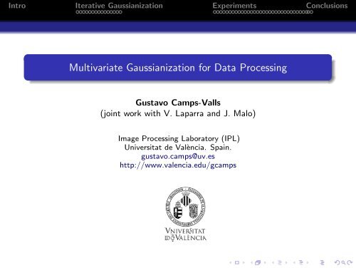
Intro Iterative <strong>Gaussianization</strong> Experiments Conclusions<strong>Multivariate</strong> <strong>Gaussianization</strong> <strong>for</strong> <strong>Data</strong> <strong>Processing</strong>Gustavo Camps-Valls(joint work with V. Laparra and J. Malo)Image <strong>Processing</strong> Laboratory (IPL)Universitat de València. Spain.gustavo.camps@uv.eshttp://www.valencia.edu/gcamps
Intro Iterative <strong>Gaussianization</strong> Experiments ConclusionsOutline1 IntroductionWhy <strong>Gaussianization</strong>?How <strong>Gaussianization</strong>?2 Iterative <strong>Gaussianization</strong> FrameworkNotation and preliminariesThe ideaTheoretical ConvergenceInvertibilityDifferentiability3 Experimental resultsImage synthesisClassificationMulti-in<strong>for</strong>mation estimation4 Conclusions
Intro Iterative <strong>Gaussianization</strong> Experiments Conclusions<strong>Gaussianization</strong>“Trans<strong>for</strong>m multidimensional data into multivariate Gaussian data”Why?Achieve statistical independence of data components is useful to ...... process dimensions independently... alleviate the curse of dimensionality... tackle the PDF estimation problem directly... apply/design methods that assume Gaussianity safely... get insight in the data characteristics
Intro Iterative <strong>Gaussianization</strong> Experiments Conclusions<strong>Gaussianization</strong>, more <strong>for</strong>mallyGiven a random variable x ∈ R d , a <strong>Gaussianization</strong> trans<strong>for</strong>m is an invertibleand differentiable trans<strong>for</strong>m G(x) such thatG(x) ∼ N (0, I)What do we need?1 Can we ‘Gaussianize’ each dimension independently?2 If not, can we look <strong>for</strong> a (hopefully linear) trans<strong>for</strong>m to do it?
Intro Iterative <strong>Gaussianization</strong> Experiments ConclusionsMarginal (univariate) <strong>Gaussianization</strong>Marginal <strong>Gaussianization</strong> is trivial [Friedman87]<strong>Gaussianization</strong> in each dimension, Ψ i (k), can be decomposed into twoconsecutive equalization trans<strong>for</strong>ms:1 Marginal uni<strong>for</strong>mization, U(k) i , based on the cdf of the marginal PDF,2 <strong>Gaussianization</strong> of a uni<strong>for</strong>m variable, G(u), based on the inverse of the cdfof a univariate Gaussian: Ψ i (k) = G ⊙ Ui (k)whereu = U i (k)(x (k)i) =G −1 (x i ) =∫ x(k)i−∞∫ xi−∞p i (x ′(k)i) dx ′(k)ig(x i ′ ) dx i′and g(x i ) is just a univariate Gaussian.0.011150.5p i(x i)0.0080.0060.004u = U i (x i)0.80.60.4p(u)0.80.60.4G(u) = Ψ i (x i)0p i(Ψ i (x i))0.40.30.20.0020.20.20.100 100 200 300x i00 100 200 300x i00 0.5 1u−50 0.5 1u0−5 0 5G(u) = Ψ i (x i)
Intro Iterative <strong>Gaussianization</strong> Experiments ConclusionsThe method is limited and may lead to a non-multivariate Gaussian distributionDesiredMarginalOriginal <strong>Gaussianization</strong> <strong>Gaussianization</strong>
Intro Iterative <strong>Gaussianization</strong> Experiments ConclusionsMotivationIdea: Rotate and Gaussianize marginally!√ An orthogonal trans<strong>for</strong>m R does not affect the measure of Gaussianity√ Univariate <strong>Gaussianization</strong> is unique up to a sign flip
Intro Iterative <strong>Gaussianization</strong> Experiments ConclusionsMotivationRBIG: Rotation-based Iterative <strong>Gaussianization</strong>Impact of different rotations: ICA, PCA, random, etc.Study of the convergenceStudy the essential propertiesInvertibilityDifferentiabilityConvergence(<strong>Multivariate</strong>) GaussianityApply it!SynthesisClassificationDependence estimation
Intro Iterative <strong>Gaussianization</strong> Experiments ConclusionsPreliminariesDefinition 1: PDF estimation under arbitrary trans<strong>for</strong>m [Stark86]Let x ∈ R d be a r.v. with PDF, p x(x). Given some bijective, differentiabletrans<strong>for</strong>m of x into y using G : R d → R d , y = G(x), the PDFs are related:p x(x) = p y(G(x))∣ dG(x)dx ∣ = py(G(x)) |∇xG(x)|where |∇ xG| is the determinant of the trans<strong>for</strong>m’s Jacobian matrix.
Intro Iterative <strong>Gaussianization</strong> Experiments ConclusionsPreliminariesDefinition 1: PDF estimation under arbitrary trans<strong>for</strong>m [Stark86]Let x ∈ R d be a r.v. with PDF, p x(x). Given some bijective, differentiabletrans<strong>for</strong>m of x into y using G : R d → R d , y = G(x), the PDFs are related:p x(x) = p y(G(x))∣ dG(x)dx ∣ = py(G(x)) |∇xG(x)|where |∇ xG| is the determinant of the trans<strong>for</strong>m’s Jacobian matrix.Remark 1The p x(x) can be obtained if the Jacobian is known, since(1p y(y) = p y(G(x)) =( √ 2π|Σ|) exp − 1 )d 2 (G(x) − µ y )⊤ Σ −1 (G(x) − µ y )
Intro Iterative <strong>Gaussianization</strong> Experiments ConclusionsPreliminariesDefinition 1: PDF estimation under arbitrary trans<strong>for</strong>m [Stark86]Let x ∈ R d be a r.v. with PDF, p x(x). Given some bijective, differentiabletrans<strong>for</strong>m of x into y using G : R d → R d , y = G(x), the PDFs are related:p x(x) = p y(G(x))∣ dG(x)dx ∣ = py(G(x)) |∇xG(x)|where |∇ xG| is the determinant of the trans<strong>for</strong>m’s Jacobian matrix.Remark 1The p x(x) can be obtained if the Jacobian is known, since(1p y(y) = p y(G(x)) =( √ 2π|Σ|) exp − 1 )d 2 (G(x) − µ y )⊤ Σ −1 (G(x) − µ y )Remark 2We need differentiable (<strong>Gaussianization</strong>) trans<strong>for</strong>ms <strong>for</strong> PDF estimation.
Intro Iterative <strong>Gaussianization</strong> Experiments ConclusionsPreliminariesDefinition 2: Iterative <strong>Gaussianization</strong> Trans<strong>for</strong>mGiven a d-dimensional random variable x (0) = [x 1, . . . , x d ] ⊤ with PDF p(x (0) ),in each iteration k, a two-step processing is per<strong>for</strong>med:G : x (k+1) = R (k) Ψ (k) (x (k) )whereΨ (k) is the marginal <strong>Gaussianization</strong> of each dimension of x (k) <strong>for</strong> thecorresponding iteration,R (k) is a rotation matrix <strong>for</strong> the marginally Gaussianized variable Ψ (k) (x (k) ).
Intro Iterative <strong>Gaussianization</strong> Experiments ConclusionsPropertiesProperty 1: The iterative <strong>Gaussianization</strong> trans<strong>for</strong>m is invertibleGiven the <strong>Gaussianization</strong> trans<strong>for</strong>m:G : x (k+1) = R (k) Ψ (k) (x (k) )by simple manipulation, the inversion trans<strong>for</strong>m is:G −1 : x (k) = Ψ −1(k) (R⊤ (k)x (k+1) ).
Intro Iterative <strong>Gaussianization</strong> Experiments ConclusionsPropertiesProperty 1: The iterative <strong>Gaussianization</strong> trans<strong>for</strong>m is invertibleGiven the <strong>Gaussianization</strong> trans<strong>for</strong>m:G : x (k+1) = R (k) Ψ (k) (x (k) )by simple manipulation, the inversion trans<strong>for</strong>m is:G −1 : x (k) = Ψ −1(k) (R⊤ (k)x (k+1) ).Remark 1: valid <strong>for</strong> any rotation trans<strong>for</strong>mInvertibility is possible <strong>for</strong> any rotation matrix R (k) .
Intro Iterative <strong>Gaussianization</strong> Experiments ConclusionsPropertiesProperty 1: The iterative <strong>Gaussianization</strong> trans<strong>for</strong>m is invertibleGiven the <strong>Gaussianization</strong> trans<strong>for</strong>m:G : x (k+1) = R (k) Ψ (k) (x (k) )by simple manipulation, the inversion trans<strong>for</strong>m is:G −1 : x (k) = Ψ −1(k) (R⊤ (k)x (k+1) ).Remark 1: valid <strong>for</strong> any rotation trans<strong>for</strong>mInvertibility is possible <strong>for</strong> any rotation matrix R (k) .Remark 2: valid <strong>for</strong> PDF connected supportInvertibility of Ψ (k) is trivially ensured when the PDF support is connected, i.e.no disjoint subspaces in the PDF support.
Intro Iterative <strong>Gaussianization</strong> Experiments ConclusionsPropertiesProperty 2: The iterative <strong>Gaussianization</strong> trans<strong>for</strong>m is differentiableThe Jacobian of the series of K iterations is the product of the Jacobians:∇ xG = ∏ Kk=1 R (k)∇ x (k)Ψ (k)Marg. Gauss. Ψ (k) is a dimension-wise trans<strong>for</strong>m with diagonal Jacobian:⎛⎞∂Ψ 1 (k)· · · 0∂x (k)1∇ x (k)Ψ (k) =⎜.⎝. ... ..⎟⎠0 · · ·Each element in ∇ x (k)Ψ (k) is:∂Ψ d (k)∂x (k)d∂Ψ i (k)∂x (k)i= ∂G∂u∂u∂x (k)i( ∂G−1=∂x i) −1p i (x (k)i) = g(Ψ i (k)(x (k)i)) −1 p i (x (k)i)
Intro Iterative <strong>Gaussianization</strong> Experiments ConclusionsPropertiesProperty 2: The iterative <strong>Gaussianization</strong> trans<strong>for</strong>m is differentiableThe Jacobian of the series of K iterations is the product of the Jacobians:∇ xG = ∏ Kk=1 R (k)∇ x (k)Ψ (k)Marg. Gauss. Ψ (k) is a dimension-wise trans<strong>for</strong>m with diagonal Jacobian:⎛⎞∂Ψ 1 (k)· · · 0∂x (k)1∇ x (k)Ψ (k) =⎜.⎝. ... ..⎟⎠0 · · ·Each element in ∇ x (k)Ψ (k) is:∂Ψ d (k)∂x (k)d∂Ψ i (k)∂x (k)i= ∂G∂u∂u∂x (k)i( ∂G−1=∂x i) −1p i (x (k)i) = g(Ψ i (k)(x (k)i)) −1 p i (x (k)i)Remark 1: rotation-independentThe differentiable nature of G is independent of the selected rotations R (k) .
Intro Iterative <strong>Gaussianization</strong> Experiments ConclusionsPropertiesQ: Does the method converge? At what rate?How to measure our distance to a unit multivariate Gaussian?
Intro Iterative <strong>Gaussianization</strong> Experiments ConclusionsPropertiesQ: Does the method converge? At what rate?How to measure our distance to a unit multivariate Gaussian?A: In<strong>for</strong>mation theory basicsNegentropy: distance to a zero mean unit multivariate GaussianMulti-in<strong>for</strong>mation: Compute the in<strong>for</strong>mation reduction after each step
Intro Iterative <strong>Gaussianization</strong> Experiments ConclusionsPropertiesDefinition 3: NegentropyNegentropy measures Gaussianity with the KLD:)J(x) = D KL(p(x)|N (µ x , σ 2 xI)Remark 1Negentropy is always non-negative and zero iff x has a Gaussian distribution
Intro Iterative <strong>Gaussianization</strong> Experiments ConclusionsPropertiesDefinition 3: NegentropyNegentropy measures Gaussianity with the KLD:)J(x) = D KL(p(x)|N (µ x , σ 2 xI)Remark 1Negentropy is always non-negative and zero iff x has a Gaussian distributionDefinition 4: Negentropy to unit GaussianKLD to a multivariate zero mean unit variance Gaussian distribution:J(x) = D KL (p(x)|N (0, I))
Intro Iterative <strong>Gaussianization</strong> Experiments ConclusionsPropertiesDefinition 3: NegentropyNegentropy measures Gaussianity with the KLD:)J(x) = D KL(p(x)|N (µ x , σ 2 xI)Remark 1Negentropy is always non-negative and zero iff x has a Gaussian distributionDefinition 4: Negentropy to unit GaussianKLD to a multivariate zero mean unit variance Gaussian distribution:J(x) = D KL (p(x)|N (0, I))Definition 5: Marginal negentropy to unit GaussianMarginal negentropy is defined as the sum of the KLDs of each marginal,p i (x i ), to the univariate zero mean unit variance Gaussian, N (0, 1):J m(x) =d∑D KL (p i (x i )|N (0, 1))i=1
Intro Iterative <strong>Gaussianization</strong> Experiments ConclusionsPropertiesDefinition 6: Multi-in<strong>for</strong>mationMulti-in<strong>for</strong>mation is the KLD between the joint PDF of a multidimensionalrandom variable and the product of its marginal PDFs [Studeny98]:I (x) = D KL (p(x)| ∏ i p i(x i ))Remark 1To assess the statistical relations among the dimensions of a random variableRemark 2Multi-in<strong>for</strong>mation generalizes mutual info. to multidimensional vectorsZero iff the different components of x are independent
Intro Iterative <strong>Gaussianization</strong> Experiments ConclusionsPropertiesTheorem 1: negentropy reduces independently of the rotation∆J = J(x) − J(RΨ(x)) ≥ 0, ∀ RProof.Divergence to a factorized PDF written in terms of its marginal PDFs [Cardoso03]:D KL (p(x) | ∏ i q i(x i )) = D KL (p(x) | ∏ i p i(x i )) + D KL ( ∏ i p i(x i ) | ∏ i q i(x i ))= I (x) + D KL ( ∏ i p i(x i ) | ∏ i q i(x i ))If q i (x i ) are univariate Gaussian PDFs, ∏ i q i(x i ) = N (0, I), and then:J(x) = I (x) + J m(x)The negentropy reduction in our trans<strong>for</strong>m is:∆J = J(x) − J(RΨ(x)) = J(x) − J(Ψ(x))= I (x) + J m(x) − I (Ψ(x)) − J m(Ψ(x)) = J m(x) ≥ 0, ∀ Rsince: (1) N (0, I) is rotation invariant; (2) the I is invariant under dim-wisetrans<strong>for</strong>ms [Studeny98]; and (3) the J m of a marginally Gaussianized r.v. is 0.
Intro Iterative <strong>Gaussianization</strong> Experiments ConclusionsPropertiesTheorem 2: redundacy reduces independently of the rotationGiven a marginally Gaussianized variable, Ψ(x), any rotation reduces theredundancy:∆I = I (Ψ(x)) − I (RΨ(x)) ≥ 0, ∀ RProof.RememberJ(x) = I (x) + J m(x) → I (x) = J(x) − J m(x)Apply it on I (Ψ(x)) and I (RΨ(x)):∆I = J(Ψ(x)) − J m(Ψ(x)) − J(RΨ(x)) + J m(RΨ(x))= J m(RΨ(x)) ≥ 0, ∀ Rsince (1) negentropy is rotation invariant, and (2) the marginal negentropy of amarginally Gaussianized r.v. is 0.
Intro Iterative <strong>Gaussianization</strong> Experiments ConclusionsPropertiesCorollary 1: convergence ensuredThe combination of marginal <strong>Gaussianization</strong> and rotation gives rise toredundancy reduction since marginal <strong>Gaussianization</strong> does not changeredundancy, I (Ψ(x)) = I (x).
Intro Iterative <strong>Gaussianization</strong> Experiments ConclusionsPropertiesCorollary 1: convergence ensuredThe combination of marginal <strong>Gaussianization</strong> and rotation gives rise toredundancy reduction since marginal <strong>Gaussianization</strong> does not changeredundancy, I (Ψ(x)) = I (x).Corollary 2: mutual and negentropy are relatedNegentropy reduction at some iteration k is related to the amount ofredundancy reduction obtained in k − 1:∆J (k) = J m(x (k) ) = ∆I (k−1)
Intro Iterative <strong>Gaussianization</strong> Experiments ConclusionsOn the suitable rotationWhich is the suitable rotation?Closed-<strong>for</strong>m Theoretical Convergence Comput.Rotation convergence√rate costICA√×√Max ∆J O(2md(d + 1)n)PCA√√∆J = 2nd order O(d 2 (d + 1)n)RND∆J ≥ 0 O(d 3 )n samples of dimension d, FastICA running m iterationsICA guarantees the theoretical convergence of the <strong>Gaussianization</strong> processsince it seeks <strong>for</strong> the maximally non-Gaussian marginal PDFsPCA leads to non-optimal convergence rate because it does reduceredundancy to a certain extent (it removes correlation), but it does notmaximize the marginal non-Gaussianity J m(x)PCA is closed-<strong>for</strong>m and is faster than ICAPCA require more iterations but Gaussianizes fasterUsing RND trans<strong>for</strong>ms guarantees the theoretical convergence, butconverges slowly
Intro Iterative <strong>Gaussianization</strong> Experiments ConclusionsOn the suitable rotationConvergence analysis1.5∆ I (bpp)10.5mance of G-PCA in a toy example. Original and trans<strong>for</strong>med data (top), and cumulati05 10 15 20 25 30 35 40iterationCA (solid) Similar and GICA convergence (dashed). rates Optimal when using iterations PCA are (solid) highlighted. or ICA (dashed) Inset scatter plots shoat different iterations.Using PCA requires more iterations to converge, but it is much faster!3. RELATION OF G-PCA TO OTHER METHODSwe point out some particularly interesting relations of the proposed G-PCA to th
Intro load, as PCA Iterative is much <strong>Gaussianization</strong> cheaper than ICA. The computational Experiments cost of FastICA is ConclusionsO(2k(d + 1)n),dimensionality, n is the number of samples, and k is the number of iterations until convergenceOn the suitable eventually rotation very high. On the other hand, PCA is basically a singular value decomposition thaO(dn 2 ) if the naïve Jacobi’s method is implemented. Note, however, that typically k ≫ n/2? Tis more relevant in higher dimensional problems. MENUDO CHARCO! To assess this, we Gaussiof different sizes from the standard grayscale image ‘Barbara’. Results <strong>for</strong> both CPU time and thare presented in Table 1. For similar ∆I reductions, more than one order of magnitude in comis gained by G-PCA, e.g. when working with 64 dimensions, G-PCA takes about 4 minutes whiComputational around 4 hours. cost analysisG-ICAG-PCAdim ∆I [bpp] Time [s] ∆I [bpp] Time [s]2 × 2 1.54 865 1.51 143 × 3 2.08 1236 2.05 344 × 4 2.38 2197 2.29 635 × 5 2.50 3727 2.44 996 × 6 2.60 6106 2.56 1417 × 7 2.68 9329 2.63 1708 × 8 2.69 15085 2.69 233Table 1. Cumulative ∆I and CPU time <strong>for</strong> G-ICA and G-PCA.Gaussianized patches of different sizes <strong>for</strong> the image ‘Barbara’More than one order of magnitude gained <strong>for</strong> similar ∆I reductions8×8 patches: 4 minutes vs 4 hours!
Intro Iterative <strong>Gaussianization</strong> Experiments ConclusionsExperiment 1: Density estimation toy examplesDensity estimation in high-dimensional problemsUnivariate density estimation is solved:Kernel estimatorsRadial basis function estimatesGaussian mixture modelsWavelet density estimates...High-dimensional density estimation is difficult!Parametric models: e.g. histogram-based→ Many samples needed, curse of dimensionalityNon-parametric models: e.g. Gaussian, GSM, etc.→ knowledge about the PDF
Intro Iterative <strong>Gaussianization</strong> Experiments ConclusionsExperiment 1: Density estimation toy examplesDensity estimation with RBIG1: Input: Given data x (0) = [x 1, . . . , x d ] ⊤ ∈ R d2: Learn the sequence of <strong>Gaussianization</strong> trans<strong>for</strong>ms, G, such that y = G(x)3: Compute its Jacobian, J G4: The p y(y) is a multivariate Gaussian:(1p y(y) = p y(G(x)) =( √ 2π|Σ|) exp − 1 )d 2 (G(x) − µ y) ⊤ Σ −1 (G(x) − µ y )5: Compute the probability in the input space with:p x(x) = p y(y) · |∇ xG|
Intro Iterative <strong>Gaussianization</strong> Experiments ConclusionsExperiment 1: Density estimation toy examplesDensity estimation with RBIG1: Input: Given data x (0) = [x 1, . . . , x d ] ⊤ ∈ R d2: Learn the sequence of <strong>Gaussianization</strong> trans<strong>for</strong>ms, G, such that y = G(x)3: Compute its Jacobian, J G4: The p y(y) is a multivariate Gaussian:(1p y(y) = p y(G(x)) =( √ 2π|Σ|) exp − 1 )d 2 (G(x) − µ y) ⊤ Σ −1 (G(x) − µ y )5: Compute the probability in the input space with:p x(x) = p y(y) · |∇ xG|AdvantagesRobustness to high dimensional problemsNo data distribution assumptions, no parametric model eitherLow computational cost
Intro Iterative <strong>Gaussianization</strong> Experiments ConclusionsExperiment 1: Density estimation toy examplesToy exampleTheoretical PDF Scatter plot Histogram G-PCA PDFe 3. Example of 10PDF 2 samples estimation. usedFrom left to right: theoretical PDF, scatter plot of the data used in the estimaram estimation Much usingsmoother a number of estimation bins to obtain the same resolution as in the G-PCA estimation.5. EXPERIMENTAL RESULTSroposed method is illustrated in two experiments and will be compared to standard SVDD because ofive similarity (cf. Section 3.1). The first 2D experiment on synthetic data illustrates the capabilities ood in non-linearly separable and badly sampled one-class problems. The second experiment deals withspectral and multisource data and illustrates the advantages of G-PCA in real and challenging scenarExperiment 1: 2D non-linearly separable problems.is 2D experiment the problem is detecting outliers from the target class represented by dots in Fig. 4.
Intro Iterative <strong>Gaussianization</strong> Experiments ConclusionsExperiment 1: Density estimation toy examplesToy exampleTheoretical PDF Scatter plot Histogram G-PCA PDFe 3. Example of 10PDF 2 samples estimation. usedFrom left to right: theoretical PDF, scatter plot of the data used in the estimaram estimation Much usingsmoother a number of estimation bins to obtain the same resolution as in the G-PCA estimation.Problems and limitations 5. EXPERIMENTAL RESULTSroposed method We need is illustrated to ensure in two connected experiments supports and will <strong>for</strong>be the compared PDF to standard SVDD because ofive similarity (cf. Section 3.1). The first 2D experiment on synthetic data illustrates the capabilities ood in non-linearly For clustered separabledata, and badly estimate sampled individual one-class trans<strong>for</strong>ms problems. <strong>for</strong> The each second cluster experiment deals withspectral andThe multisource Jacobian data estimation and illustrates is highly the advantages point-dependent of G-PCA in real and challenging scenarExperiment 1: 2D non-linearly separable problems.is 2D experiment the problem is detecting outliers from the target class represented by dots in Fig. 4.
Intro Iterative <strong>Gaussianization</strong> Experiments ConclusionsExperiment 1: Density estimation toy examplesG-PCAToy example 2: convergence to a multivariate Gaussian. Original <strong>Data</strong>
Intro Iterative <strong>Gaussianization</strong> Experiments ConclusionsExperiment 1: Density estimation toy examplesG-PCAk=1
Intro Iterative <strong>Gaussianization</strong> Experiments ConclusionsExperiment 1: Density estimation toy examplesG-PCAk=2
Intro Iterative <strong>Gaussianization</strong> Experiments ConclusionsExperiment 1: Density estimation toy examplesG-PCAk=3
Intro Iterative <strong>Gaussianization</strong> Experiments ConclusionsExperiment 1: Density estimation toy examplesG-PCAk=4
Intro Iterative <strong>Gaussianization</strong> Experiments ConclusionsExperiment 1: Density estimation toy examplesG-PCAk=8
Intro Iterative <strong>Gaussianization</strong> Experiments ConclusionsExperiment 1: Density estimation toy examplesG-PCAk=9
Intro Iterative <strong>Gaussianization</strong> Experiments ConclusionsExperiment 1: Density estimation toy examplesG-PCAk=10
Intro Iterative <strong>Gaussianization</strong> Experiments ConclusionsExperiment 1: Density estimation toy examplesG-PCAk=13
Intro Iterative <strong>Gaussianization</strong> Experiments ConclusionsExperiment 1: Density estimation toy examplesG-PCAk=15
Intro Iterative <strong>Gaussianization</strong> Experiments ConclusionsExperiment 1: Density estimation toy examplesG-PCAk=18
Intro Iterative <strong>Gaussianization</strong> Experiments ConclusionsExperiment 1: Density estimation toy examplesG-PCAk=20
Intro Iterative <strong>Gaussianization</strong> Experiments ConclusionsExperiment 1: Density estimation toy examplesG-PCAk=24. Gaussianized!
Intro Iterative <strong>Gaussianization</strong> Experiments ConclusionsExperiment 2: <strong>Data</strong> synthesis‘<strong>Data</strong> synthesis allows one togenerate artificial data with similarstatistical properties to real data’Image synthesisTexture synthesisSpeech synthesisetc.2/ Síntesis de texturas2/ Síntesis de texturas7474
Intro Iterative <strong>Gaussianization</strong> Experiments ConclusionsExperiment 2: <strong>Data</strong> synthesis<strong>Data</strong> synthesis with RBIG1: Input: Given data x (0) = [x 1, . . . , x d ] ⊤ ∈ R d2: Learn the sequence of <strong>Gaussianization</strong> trans<strong>for</strong>ms, G, such that y = G(x)3: Compute its Jacobian, J G4: Sample randomly in the Gaussianized domain5: Trans<strong>for</strong>m back to the original domain
Intro Iterative <strong>Gaussianization</strong> Experiments ConclusionsExperiment 2: <strong>Data</strong> synthesis<strong>Data</strong> synthesis with RBIG1: Input: Given data x (0) = [x 1, . . . , x d ] ⊤ ∈ R d2: Learn the sequence of <strong>Gaussianization</strong> trans<strong>for</strong>ms, G, such that y = G(x)3: Compute its Jacobian, J G4: Sample randomly in the Gaussianized domain5: Trans<strong>for</strong>m back to the original domainAdvantagesRobustness to high dimensional problemsNo data distribution assumptions, no parametric model eitherLow computational cost
Intro Iterative <strong>Gaussianization</strong> Experiments ConclusionsExperiment 2: <strong>Data</strong> synthesisOriginal data Gaussianized data Synthesized data
Intro Iterative <strong>Gaussianization</strong> Experiments ConclusionsExperiment 2: <strong>Data</strong> synthesis
Intro Iterative <strong>Gaussianization</strong> Experiments ConclusionsExperiment 3: One-class ClassificationOne-class classificationOne-class classification tries to distinguish one class of objects from all otherpossible objects, by learning from a training set containing only the objects ofthat class.ApplicationsChange detectionAnomaly detectionTarget detectionMethodsDensity estimation methods:More complex in high dim. spacesMore accurate with high number of samplesBoundary methods, like the support vector domain description (SVDD)Robust to high dim. spacesMore accurate with low number of training samples
Intro Iterative <strong>Gaussianization</strong> Experiments ConclusionsExperiment 3: One-class ClassificationOne-class classification TOY EXAMPLE Toy example GPCA vs SVDD<strong>Gaussianization</strong> andG-PCASVDD perfectly reject outliers SVDDBoth model the class of interest• PROBLEM WITH NO TARGET SAMPLES• PROBLEM WITH THE REPRESENTATIVITY OF NO TARGET SAMPLES
Intro Iterative <strong>Gaussianization</strong> Experiments ConclusionsExperiment 3: One-class ClassificationOne-class classification TOY EXAMPLE Toy example GPCA vs SVDDSVDD has problemsG-PCAwith badly-sampled space and/or SVDDrepresentativeness of the outlier samples• PROBLEM WITH NO TARGET SAMPLES• PROBLEM WITH THE REPRESENTATIVITY OF NO TARGET SAMPLES
Intro Iterative <strong>Gaussianization</strong> Experiments ConclusionsExperiment 3: One-class ClassificationOne-class remote sensing image classificationObjetive: Detection of classes ‘urban’ vs. ‘non-urban’.‘Urban Expansion Monitoring (UrbEx) ESA-ESRIN DUP’ Project.2 sensors (ERS2 SAR y Landsat TM) in 2 dates (1995 and 1999) overRome.Features and pre-processingImages were co-registered with ISTAT data (at subpixel level,
Intro Iterative <strong>Gaussianization</strong> Experiments ConclusionsExperiment 3: One-class ClassificationBuilding the classifiersRBF kernel <strong>for</strong> the SVDD: K(x i , x j ) = exp ( −‖x i − x j ‖ 2 /2σ 2) , σ ∈ R + .Kernel width varied in σ ∈ [10 −2 , . . . , 10 2 ]The fraction rejection parameter was varied in ν ∈ [10 −2 , 0.5]Experimental setupTrain with a set of free parameters to maximize kappa statisticTraining sets of different size <strong>for</strong> the target class, [100, 2500]Test set was constituted by 10 5 pixelsExperiment repeated 10 runs in 3 images
crosses represent outliers of different nature. The figures show the classification boundaries found by SVDD (left) andIntro G-PCA (right) whenIterative trained using <strong>Gaussianization</strong> a restricted set of outliers (crosses). Experiments ConclusionsExperiment method <strong>for</strong>3: small One-class size training Classification sets. This is because more target samples are needed by the G-PCA <strong>for</strong> anaccurate PDF estimation. However, <strong>for</strong> moderate and large training sets the proposed method substantiallyoutper<strong>for</strong>ms SVDD. Note that training size requirements of G-PCA are not too demanding: 750 samples on a10-dimensional problem are enough <strong>for</strong> G-PCA to outper<strong>for</strong>m SVDD when very little is known of the non-targetclass. Classification accuracyNaples, 1995 Naples, 1999 Rome 19990.50.50.5κ statistic0.40.30.2κ statistic0.40.30.2κ statistic0.40.30.20.10.10.100 500 1000 1500 2000 2500Training samples00 500 1000 1500 2000 2500Training samplesThe estimated κ statistic jointly measures precision and recall00 500 1000 1500 2000 2500Training samplesFigure 5. Classification per<strong>for</strong>mance (κ statistics) as a function of the number of training samples <strong>for</strong> the three consideredimages by the SVDD (dashed) and the G-PCA (solid)..Results <strong>for</strong> test, 10 5 pixelsPoor results, very challenging problem:Figure 6 shows Training the classification with few samples maps using and a restricted from antraining independent strategy. area In this case, the experiment wascarried out over High a small variance region (200 of the × 200) spectral of thesignaturesNaples 1995 image. We used 2000 samples of the target classand only 10 samples of the non-target class. Here the classification per<strong>for</strong>mance (κ statistic) is better thanSVDD outper<strong>for</strong>ms RBIG <strong>for</strong> small size training setsthe results reported in Fig. 5 because small regions have more homogeneous features, and then the varianceof spectral RBIG signatures outper<strong>for</strong>ms is smaller. SVDD As a consequence, <strong>for</strong> moderate the training and large data describes trainingmore sets accurately the particularbehavior of the smaller spatial region thus achieving a better per<strong>for</strong>mance in the test set.Note that, although the SVDD classification map is more homogeneous, G-PCA better rejects the ‘nonurban’areas (in black). This may be because SVDD training with few non-target data gives rise to a too broad
Intro Iterative <strong>Gaussianization</strong> Experiments ConclusionsExperiment 3: One-class ClassificationClassification accuracy (II)Ground truth SVDD κ = 0.62 G-PCA κ = 0.65A small region (200 × 200) of the Naples 1995 image.Figure 6. Classification per<strong>for</strong>mance over a small region of the Naples image (1995). White points represent urban areaswhile black 2000 points represent samples non-urban of theareas.target class and only 10 samples of the non-targetclass <strong>for</strong> tuning parameters.Much better results (lower 6. spectral CONCLUSIONS variance)We proposed SVDD a fast alternative classification to iterative map <strong>Gaussianization</strong> is more homogeneous methods that but makes fails it suitable in outlier in high-dimensionalproblems such identificationas those in remote sensing applications. The proposed G-PCA consists of iteratively applyingmarginal <strong>Gaussianization</strong> and PCA to any original dataset. The result is a multivariate Gaussian. TheoreticalRBIG better rejects the ‘non-urban’ areas (in black)convergence of the proposed method was proved.The methodNoisyexhibits resultsfast canandbe stablesolvedconvergenceby includingrates throughspatialain<strong>for</strong>mationsuitable early-stopping criterion. Thecomputational cost is dramatically reduced compared to ICA-based <strong>Gaussianization</strong> methods. The proposed
Intro Iterative <strong>Gaussianization</strong> Experiments ConclusionsExperiment 4: Natural and remote sensing image <strong>Gaussianization</strong>
Intro Iterative <strong>Gaussianization</strong> Experiments ConclusionsExperiment 5: Multi-in<strong>for</strong>mation estimationMeasuring dependence‘Two random variables are independent if the conditional probabilitydistribution of either given the observed value of the other is the same as if theother’s value had not been observed’ApplicationsFeature selection<strong>Data</strong> analysis<strong>Data</strong> codingMany MethodsCorrelation only measures linear dependencesNon-linear extensions availableKernel methods can estimate higher-order dependencesMutual in<strong>for</strong>mation measures dependence between two r.v.’sMulti-in<strong>for</strong>mation generalizes mutual in<strong>for</strong>mation
Intro Iterative <strong>Gaussianization</strong> Experiments ConclusionsExperiment 5: Multi-in<strong>for</strong>mation estimationMeasuring independence with RBIG1: Input: Given data x (0) = [x 1, . . . , x d ] ⊤ ∈ R d2: Learn the sequence of <strong>Gaussianization</strong> trans<strong>for</strong>ms, G, such that y = G(x)3: Compute the cumulative reduction in mutual in<strong>for</strong>mation
Intro Iterative <strong>Gaussianization</strong> Experiments ConclusionsExperiment 5: Multi-in<strong>for</strong>mation estimationMeasuring independence with RBIG1: Input: Given data x (0) = [x 1, . . . , x d ] ⊤ ∈ R d2: Learn the sequence of <strong>Gaussianization</strong> trans<strong>for</strong>ms, G, such that y = G(x)3: Compute the cumulative reduction in mutual in<strong>for</strong>mationAdvantagesRobustness to high dimensional problems, no need of histograms!No data distribution assumptions, no parametric model eitherLow computational cost
Intro Iterative <strong>Gaussianization</strong> Experiments ConclusionsExperiment 5: Multi-in<strong>for</strong>mation estimationMutual in<strong>for</strong>mation estimation in nonlinear manifoldsɛ r = 100 × (I − Î )/I [%] (10 realizations)Dim3 6.97 7.87 6.304 1.50 0.31 0.485 3.53 2.97 3.288 3.13 3.69 3.7210 1.48 1.45 1.32
Intro Iterative <strong>Gaussianization</strong> Experiments ConclusionsExperiment 5: Multi-in<strong>for</strong>mation estimationMutual in<strong>for</strong>mation estimation in nonlinear manifoldsɛ r = 100 × (I − Î )/I [%] (10 realizations)Dim3 6.97 7.87 6.304 1.50 0.31 0.485 3.53 2.97 3.288 3.13 3.69 3.7210 1.48 1.45 1.32Problems and limitationsEntropy estimators are not perfectly definedMore iterations, more error: overfitting?More error with complex manifolds
Intro Iterative <strong>Gaussianization</strong> Experiments ConclusionsConclusions & Further workConclusions1 A framework <strong>for</strong> multidimensional <strong>Gaussianization</strong> presented:General: any orthogonal trans<strong>for</strong>m can be plugged inConvergence studiedInvertible and differentiable2 Useful <strong>for</strong> large scale real problems:ClassificationTarget detectionDensity estimationSynthesisSaliencyMulti-in<strong>for</strong>mation estimation
Intro Iterative <strong>Gaussianization</strong> Experiments ConclusionsConclusions & Further workConclusions1 A framework <strong>for</strong> multidimensional <strong>Gaussianization</strong> presented:General: any orthogonal trans<strong>for</strong>m can be plugged inConvergence studiedInvertible and differentiable2 Useful <strong>for</strong> large scale real problems:ClassificationTarget detectionDensity estimationSynthesisSaliencyMulti-in<strong>for</strong>mation estimationFurther workBlind source separation in multiple post-nonlinear stages?Regularization and overfitting studies in DNN?
Intro Iterative <strong>Gaussianization</strong> Experiments Conclusionshttp://isp.uv.es/soft.htmReferencesReferencesV. Laparra, G. Camps-Valls and J. Malo, “Iterative <strong>Gaussianization</strong>: fromICA to Random Rotations”. IEEE Trans. Neural Networks (2011)V. Laparra, G. Camps-Valls and J. Malo, “PCA <strong>Gaussianization</strong> <strong>for</strong> Image<strong>Processing</strong>”. ICIP (2009)V. Laparra, J. Muñoz-Marí, G. Camps-Valls and J. Malo, “PCA<strong>Gaussianization</strong> <strong>for</strong> One-Class Remote Sensing Image Classification”,SPIE: Europe Remote Sensing (2009)D. W. Scott, <strong>Multivariate</strong> Density Estimation: Theory, Practice, andVisualization, Wiley & Sons, 1992.J.H. Friedman and J.W. Tukey, “A projection pursuit algorithm <strong>for</strong>exploratory data analysis,” IEEE Trans. Comp., vol. C-23, no. 9, pp.881–890, 1974.P. J. Huber, “Projection pursuit,” The Annals of Statistics, vol. 13, no. 2,pp. 435–475, 1985.G. E. Hinton and R. R. Salakhutdinov, “Reducing the dimensionality ofdata with neural networks,” Science, 313(5786), 504–507, 2006.