Multivariate Gaussianization for Data Processing

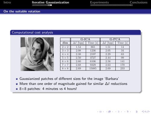
Intro load, as PCA Iterative is much Gaussianization cheaper than ICA. The computational Experiments cost of FastICA is ConclusionsO(2k(d + 1)n),dimensionality, n is the number of samples, and k is the number of iterations until convergenceOn the suitable eventually rotation very high. On the other hand, PCA is basically a singular value decomposition thaO(dn 2 ) if the naïve Jacobi’s method is implemented. Note, however, that typically k ≫ n/2? Tis more relevant in higher dimensional problems. MENUDO CHARCO! To assess this, we Gaussiof different sizes from the standard grayscale image ‘Barbara’. Results for both CPU time and thare presented in Table 1. For similar ∆I reductions, more than one order of magnitude in comis gained by G-PCA, e.g. when working with 64 dimensions, G-PCA takes about 4 minutes whiComputational around 4 hours. cost analysisG-ICAG-PCAdim ∆I [bpp] Time [s] ∆I [bpp] Time [s]2 × 2 1.54 865 1.51 143 × 3 2.08 1236 2.05 344 × 4 2.38 2197 2.29 635 × 5 2.50 3727 2.44 996 × 6 2.60 6106 2.56 1417 × 7 2.68 9329 2.63 1708 × 8 2.69 15085 2.69 233Table 1. Cumulative ∆I and CPU time for G-ICA and G-PCA.Gaussianized patches of different sizes for the image ‘Barbara’More than one order of magnitude gained for similar ∆I reductions8×8 patches: 4 minutes vs 4 hours!