Effect of Hub Motor Mass on Stability and Comfort ... - Protean Electric
Effect of Hub Motor Mass on Stability and Comfort ... - Protean Electric
Effect of Hub Motor Mass on Stability and Comfort ... - Protean Electric

Create successful ePaper yourself
Turn your PDF publications into a flip-book with our unique Google optimized e-Paper software.
The two forces Fv <strong>and</strong> Fs, which are the forces acting <strong>on</strong> the<br />
sprung <strong>and</strong> unsprung mass respectively can be found through<br />
inspecti<strong>on</strong> <str<strong>on</strong>g>of</str<strong>on</strong>g> Fig. 1. The dynamic equati<strong>on</strong>s <str<strong>on</strong>g>of</str<strong>on</strong>g> the system<br />
become:<br />
= −K<br />
S ( z − y)<br />
− BS<br />
( z − y)<br />
− M g<br />
(3)<br />
= K ( z − y)<br />
+ B ( z − y)<br />
− K ( y − x)<br />
− B ( y − x)<br />
− M g (4)<br />
MV z<br />
V<br />
M S y S<br />
S<br />
T<br />
T<br />
S<br />
C. Wheel Hop<br />
A very real phenomen<strong>on</strong> is that <str<strong>on</strong>g>of</str<strong>on</strong>g> the tire losing c<strong>on</strong>tact<br />
with the road surface, also known as “wheel hop”. This<br />
phenomen<strong>on</strong> needs to be taken into account as it could happen<br />
during the simulati<strong>on</strong>s that the tire looses c<strong>on</strong>tact with the<br />
road due to either fast changing road c<strong>on</strong>diti<strong>on</strong>s or the<br />
instability <str<strong>on</strong>g>of</str<strong>on</strong>g> the suspensi<strong>on</strong> system.<br />
The last point <str<strong>on</strong>g>of</str<strong>on</strong>g> c<strong>on</strong>tact between the tire <strong>and</strong> the road surface<br />
occurs when the unsprung mass <strong>and</strong> the road surface is<br />
equally displaced from their respective origins i.e. y-x=0. The<br />
force due to the tire spring <strong>and</strong> damper are <strong>on</strong>ly exerted when<br />
the wheel is in c<strong>on</strong>tact with the road surface. Incorporating<br />
wheel hop into the dynamic equati<strong>on</strong>s, (4) becomes:<br />
= K S ( z − y)<br />
+ BS<br />
( z − y)<br />
− KT<br />
( y − x)<br />
− BS<br />
( y − x)<br />
− M g (5)<br />
if ( y − x)<br />
≤ 0<br />
= K S ( z − y)<br />
+ BS<br />
( z − y)<br />
− M g<br />
(6)<br />
if ( y − x)<br />
≥ 0<br />
M S y<br />
S<br />
M S y<br />
S<br />
The wheel hop phenomen<strong>on</strong> adds a n<strong>on</strong>-linearity to the<br />
system. It has been decided that it can be neglected during the<br />
frequency analysis <str<strong>on</strong>g>of</str<strong>on</strong>g> the system, but not for the simulati<strong>on</strong>s.<br />
It will have little or no effect <strong>on</strong> the frequency resp<strong>on</strong>se <str<strong>on</strong>g>of</str<strong>on</strong>g> the<br />
system. It adds complexity to the analysis with little increase<br />
in the accuracy <str<strong>on</strong>g>of</str<strong>on</strong>g> the results.<br />
D. Vehicle Parameters<br />
Two vehicles are compared in the study. One is a<br />
st<strong>and</strong>ard vehicle <strong>and</strong> the other a vehicle with a hub motor<br />
place in the rear wheels. The same total mass i.e. sprung <strong>and</strong><br />
unsprung mass combined, is used for both vehicles. A total<br />
mass <str<strong>on</strong>g>of</str<strong>on</strong>g> 1500 kg was chosen. This is the mass <str<strong>on</strong>g>of</str<strong>on</strong>g> a fully laden<br />
vehicle (vehicle mass, passengers <strong>and</strong> payload). All c<strong>on</strong>stants<br />
used, such as damping <strong>and</strong> spring coefficients, are kept the<br />
same for both vehicles. Table I gives a list <str<strong>on</strong>g>of</str<strong>on</strong>g> all the c<strong>on</strong>stants<br />
used.<br />
TABLE I<br />
VEHICLE PARAMETERS<br />
St<strong>and</strong>ard Vehicle <str<strong>on</strong>g>Hub</str<strong>on</strong>g> Driven Vehicle<br />
Total Model Total Model<br />
Total <str<strong>on</strong>g>Mass</str<strong>on</strong>g> (kg) 1500 375 1500 375<br />
Sprung mass (kg) 1340 335 1100 275<br />
Unsprung mass (kg) 160 40 400 100<br />
Ks (N/m) 36 000 36 000 36 000 36 000<br />
Bs (Ns/m) 3000 3000 3000 3000<br />
Kt (N/m) 110 000 110 000 110 000 110 000<br />
Bt (Ns/m) 200 200 200 200<br />
The st<strong>and</strong>ard vehicle will serve as the c<strong>on</strong>trol for the<br />
investigati<strong>on</strong> <strong>and</strong> the hub driven vehicle as the experiment. As<br />
the simulati<strong>on</strong> uses the quarter vehicle suspensi<strong>on</strong> model, all<br />
masses are a quarter <str<strong>on</strong>g>of</str<strong>on</strong>g> the real values.<br />
III. FREQUENCY ANALYSIS<br />
A. Bode-plot Analysis<br />
It is important to verify that the suspensi<strong>on</strong> system <strong>and</strong><br />
the vehicle are, through system frequency resp<strong>on</strong>se analysis,<br />
stabile under changing road surface c<strong>on</strong>diti<strong>on</strong>s. The simplest<br />
method to investigate the frequency resp<strong>on</strong>se <str<strong>on</strong>g>of</str<strong>on</strong>g> the system is<br />
through a Bode-plot analysis. This can easily be d<strong>on</strong>e with the<br />
help <str<strong>on</strong>g>of</str<strong>on</strong>g> s<str<strong>on</strong>g>of</str<strong>on</strong>g>tware like MatLab.<br />
The transfer functi<strong>on</strong> is required to obtain the Bode-plot <str<strong>on</strong>g>of</str<strong>on</strong>g> the<br />
system. The transfer functi<strong>on</strong> can be mathematically derived<br />
from the dynamic equati<strong>on</strong>s or extracted from the linear model<br />
using MatLab. From MatLab the transfer functi<strong>on</strong> for the<br />
st<strong>and</strong>ard vehicle system is given as<br />
( s)<br />
G ST<br />
3<br />
2<br />
8.<br />
527e<br />
−14s<br />
+ 4.<br />
093e<br />
−12s<br />
+ 2.<br />
463e4s<br />
+ 2.<br />
955e5<br />
= (7)<br />
4<br />
3 2<br />
s + 88.<br />
96s<br />
+ 3802s<br />
+ 2.<br />
516e4s<br />
+ 2.<br />
955e5<br />
<strong>and</strong> the hub driven vehicle system as<br />
( s)<br />
G HD<br />
3<br />
6.<br />
395e<br />
−14s<br />
+ 3.<br />
638e<br />
−12s<br />
+ 1.<br />
2e4s<br />
+ 1.<br />
44e5<br />
= (8)<br />
4<br />
3 2<br />
s + 42.<br />
91s<br />
+ 1613s<br />
+ 1.<br />
226e4s<br />
+ 1.<br />
44e5<br />
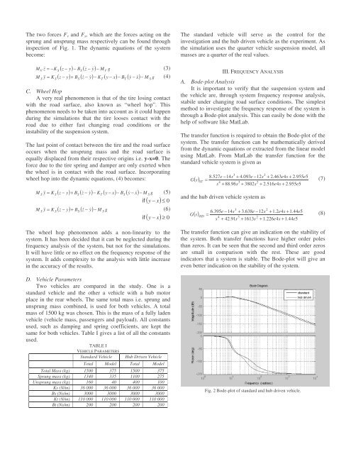
The transfer functi<strong>on</strong> can give an indicati<strong>on</strong> <strong>on</strong> the stability <str<strong>on</strong>g>of</str<strong>on</strong>g><br />
the system. Both transfer functi<strong>on</strong>s have higher order poles<br />
than zeros. It can be seen that the sec<strong>on</strong>d <strong>and</strong> third order zeros<br />
are small in comparis<strong>on</strong> with the rest. These are good<br />
indicators that a system is stable. The Bode-plot will give an<br />
even better indicati<strong>on</strong> <strong>on</strong> the stability <str<strong>on</strong>g>of</str<strong>on</strong>g> the system.<br />
Fig. 2 Bode-plot <str<strong>on</strong>g>of</str<strong>on</strong>g> st<strong>and</strong>ard <strong>and</strong> hub driven vehicle.<br />
2