Effect of Hub Motor Mass on Stability and Comfort ... - Protean Electric

Frequency (Hz)
2.8
2.6
2.4
2.2
2
1.8
1.6
1.4
1.2
1
0 100 200 300 400 500 600 700
Standard
<strong>Hub</strong>-driven
Payload (kg)
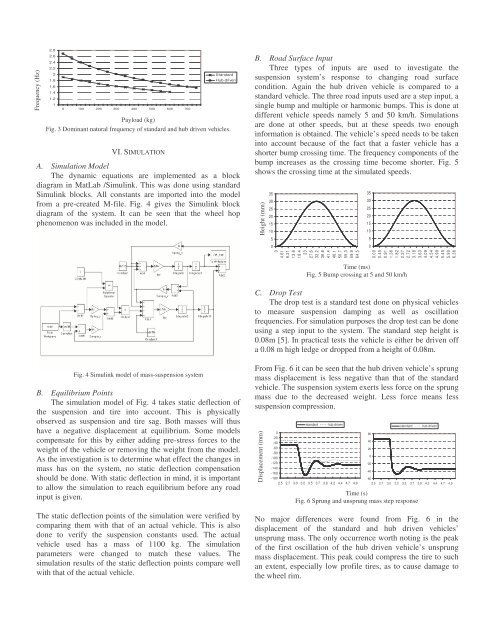
Fig. 3 Dominant natural frequency <strong>of</strong> standard and hub driven vehicles.
VI. SIMULATION
A. Simulation Model
The dynamic equations are implemented as a block
diagram in MatLab /Simulink. This was done using standard
Simulink blocks. All constants are imported into the model
from a pre-created M-file. Fig. 4 gives the Simulink block
diagram <strong>of</strong> the system. It can be seen that the wheel hop
phenomenon was included in the model.
Fig. 4 Simulink model <strong>of</strong> mass-suspension system
B. Equilibrium Points
The simulation model <strong>of</strong> Fig. 4 takes static deflection <strong>of</strong>
the suspension and tire into account. This is physically
observed as suspension and tire sag. Both masses will thus
have a negative displacement at equilibrium. Some models
compensate for this by either adding pre-stress forces to the
weight <strong>of</strong> the vehicle or removing the weight from the model.
As the investigation is to determine what effect the changes in
mass has on the system, no static deflection compensation
should be done. With static deflection in mind, it is important
to allow the simulation to reach equilibrium before any road
input is given.
The static deflection points <strong>of</strong> the simulation were verified by
comparing them with that <strong>of</strong> an actual vehicle. This is also
done to verify the suspension constants used. The actual
vehicle used has a mass <strong>of</strong> 1100 kg. The simulation
parameters were changed to match these values. The
simulation results <strong>of</strong> the static deflection points compare well
with that <strong>of</strong> the actual vehicle.
B. Road Surface Input
Three types <strong>of</strong> inputs are used to investigate the
suspension system’s response to changing road surface
condition. Again the hub driven vehicle is compared to a
standard vehicle. The three road inputs used are a step input, a
single bump and multiple or harmonic bumps. This is done at
different vehicle speeds namely 5 and 50 km/h. Simulations
are done at other speeds, but at these speeds two enough
information is obtained. The vehicle’s speed needs to be taken
into account because <strong>of</strong> the fact that a faster vehicle has a
shorter bump crossing time. The frequency components <strong>of</strong> the
bump increases as the crossing time become shorter. Fig. 5
shows the crossing time at the simulated speeds.
Height (mm)
35
30
25
20
15
10
5
0
0
4.61
9.21
13.8
18.4
23
27.6
32.2
36.8
41.4
46.1
50.7
55.3
59.9
64.5
Time (ms)
Fig. 5 Bump crossing at 5 and 50 km/h
35
30
25
20
15
10
5
0
0.00
0.45
0.91
1.36
1.82
2.27
2.72
3.18
3.63
4.09
4.54
4.99
5.45
5.90
6.36
C. Drop Test
The drop test is a standard test done on physical vehicles
to measure suspension damping as well as oscillation
frequencies. For simulation purposes the drop test can be done
using a step input to the system. The standard step height is
0.08m [5]. In practical tests the vehicle is either be driven <strong>of</strong>f
a 0.08 m high ledge or dropped from a height <strong>of</strong> 0.08m.
From Fig. 6 it can be seen that the hub driven vehicle’s sprung
mass displacement is less negative than that <strong>of</strong> the standard
vehicle. The suspension system exerts less force on the sprung
mass due to the decreased weight. Less force means less
suspension compression.
Displacement (mm)
standard hub driven
0
-20
-40
-60
-80
-100
-120
-140
-160
-180
2.5 2.7 3.0 3.2 3.5 3.7 3.9 4.2 4.4 4.7 4.9
60
40
20
0
-20
-40
standard hub driven
-60
2.5 2.7 3.0 3.2 3.5 3.7 3.9 4.2 4.4 4.7 4.9
Time (s)
Fig. 6 Sprung and unsprung mass step response
No major differences were found from Fig. 6 in the
displacement <strong>of</strong> the standard and hub driven vehicles’
unsprung mass. The only occurrence worth noting is the peak
<strong>of</strong> the first oscillation <strong>of</strong> the hub driven vehicle’s unsprung
mass displacement. This peak could compress the tire to such
an extent, especially low pr<strong>of</strong>ile tires, as to cause damage to
the wheel rim.