application switching

WHITE PAPER: WP011
Selecting eGaN® FET Optimal On-Resistance
Selecting eGaN® FET Optimal
On-Resistance
EFFICIENT POWER CONVERSION
Johan Strydom, Ph.D., V.P., Applications, Efficient Power Conversion Corporation (www.epc-co.com)
In this white paper the die size optimization process for selecting the eGaN FET optimal on-resistance is discussed and an example application
is used to show specific results. Since ‘optimum’ means different things to different people, this process is aimed at maximizing switching
device efficiency at a given load condition.
Device Losses Modeling
Previously published articles showed that eGaN FETs behave for the most part just like silicon devices and can be evaluated using similar performance metrics. Since
these devices behave like silicon MOSFETs, they can also be optimized in a similar fashion; by balancing static and dynamic losses through adjusting die size. Static
losses include loss components unaffected by changes in switching frequency, while dynamic losses are very much frequency dependent. An assumption is that all
device parameters will scale with die size but that the device Figures of Merit (FOMs) will remain unchanged. Although applications may be varied, the different loss
components are easily summarized [3, 4, 5]; only their relative sizes change with application and operating frequency. With eGaN FETs, the relative weights of the loss
components will also differ from silicon MOSFETs and thus result in different ‘optimum’ die size values. To better understand this, lets first break down the total semiconductor
losses within a power FET (P SEMI
) as follows:
where:
P SEMI
= P COND
+ P DIODE
+ P T-ON
+ P T-OFF
+ P DR
+ P QRR
+ P QOSS (1)
1 P COND is the device channel conduction loss when on
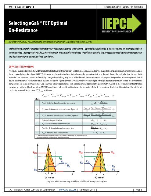
2a P T-ON is the device turn-on commutation loss (Figure 1a)
2b P T-OFF is the device turn-off commutation loss (Figure 1b)
3 P DR is the device gate drive loss
4 P QRR is the device diode reverse recovery loss
5 P QOSS is the device output capacitance charge loss
6 P DIODE is the device diode conduction loss
‘A’ refers to the normalized die area and subscript A refers to the parameter per normalized die area.
See appendix for terms, assumptions and approximations made.
( I ⋅ D )
2 RDS
( ON ),
A
L ⋅
A
VBUS
⋅ I RG
⋅ ( Q
L
GD,
A
+ Q
GS2,A
) ⋅ A
⋅ f
2 VDR
−VPL
VBUS
⋅ I R
L G
⋅ ( QGD,
A
+ Q
GS2,A
) ⋅ A
⋅ f
2
VPL
QG, A
⋅ A ⋅ VDR
⋅ fSW
QRR,
A
⋅ A ⋅ VBUS
⋅ fSW
QOSS
, A
⋅ A
⋅ VBUS
⋅ fSW
2
I ⋅ V ⋅ ∆t
⋅ f
L
F
SW
SW
SW
V BUS
I L
I L
I DS
I DS
V GS
V V DR
DS
VDR
V PL
V PL
V TH
t r t f t
t r t f
t
(a) Turn-on
(b) Turn-off
Figure 1: Idealized switching waveforms used for calculating switching loss.
Figure 1: Idealized switching waveforms used for calculating switching loss.
V TH
V BUS
V GS
EPC – EFFICIENT POWER CONVERSION CORPORATION | WWW.EPC-CO.COM | COPYRIGHT 2013 | | PAGE 1
V DS

WHITE PAPER: WP011
Selecting eGaN® FET Optimal On-Resistance
Note that not all devices will have all these loss components, e.g. a synchronous buck converter would have practically no turn-on or turn-off losses in the synchronous
rectifier. Furthermore, to optimize multiple devices in a converter, the losses stemming from the interaction between devices also need to be considered (e.g.
the diode reverse recovery losses of one device may be dissipated in another FET. This occurs in circuits such as synchronous buck converters where synchronous FET
related losses are dissipated in the control FET, but by optimizing the control FET only, this loss component will remain unchanged. Thus for optimization purposes,
this issue is resolved by considering all the losses induced by a device to be relevant for its sizing, regardless of where the power is dissipated.
Die Size Optimization
By considering each of these device loss components in eq. (1) in turn, some conclusions can be drawn:
• The conduction losses (item 1) are frequency independent
• Commutation loss (items 2a and 2b) are both frequency and load current dependent and can be combined as follows:
where:
k k ON
+ k OFF
P
k
= ON
V
2
RG
=
V − V
BUS
COMM
= k ⋅QSW , A
DR
PL
⋅ A⋅
I
R
L
⋅ f
SW
G
k
OFF
= and Q
SW, A
= QGD,
A
+ QGS2, A
VPL
(2)
• Loss components in items 3, 4 and 5 are all frequency dependent, but current independent and can be combined. While Q RR
is current related, MOSFET vendors
neglect to present their characteristic adequately over current, temperature and di/dt to accurately calculate these losses:
(
Q
)
2
OSS,
A
P
CHARGE
= ⋅ VBUS
+ Q
G,A
⋅ VDR
+ QRR
A
⋅ VBUS
⋅ A⋅
f
,
SW
(3)
• Diode losses, item 6, are assumed die size independent (only a weak function of die size) and neglected for the optimization process.
If we now define two new variables ΔI EQ
and ΔI EQRR
as:
∆I
EQ
Q
=
OSS , A
⋅ VBUS
+ 2
V
BUS
⋅ Q
⋅ k ⋅ Q
G,A
SW,
A
⋅ V
DR
(4a)
∆I
EQRR
=
2 ⋅ Q
k ⋅ Q
RR,
A
SW , A
(4b)
Then combining eq. (2) and eq. (3) and substituting eq. (4a) and (4b), the switching losses are:
P
SW
=
=
=
[
V
(
Q
k ⋅ Q ⋅ I +
2
2
⋅ V + Q ⋅ V + Q
)]
⋅ V
[
V
V
k ⋅ Q ⋅ I +
2
2
k ⋅ Q ⋅ ( ∆I
+ ∆I
)]
⋅ A⋅
f
[
V
2
k ⋅ Q
]
⋅ ( I + ∆I
+ ∆I
) ⋅ f ⋅ A
= P
BUS
BUS
BUS
SW,
A
⋅ A
SW,
A
SW,
A
SW , A
L
L
L
OSS,
A
BUS
EQ
BUS
SW,
A
EQRR
G,A
EQ
SW
DR
EQRR
RR,
A
BUS
SW
⋅ A ⋅
f
SW
(5)
EPC – EFFICIENT POWER CONVERSION CORPORATION | WWW.EPC-CO.COM | COPYRIGHT 2013 | | PAGE 2

WHITE PAPER: WP011
Selecting eGaN® FET Optimal On-Resistance
Thus the non-current dependent losses in eq. (3) can be modeled as an equivalent switching loss with an equivalent current ΔI EQRR
for reverse recovery related losses,
and ΔI EQ
as the remaining charge related losses as defined in eq. (4). The Q RR
related losses term can be neglected for eGaN FETs where Q RR
is equal to zero, but is included
for MOSFET compatibility. Thus from eq. (5) and item 1 from eq. (1), the total device losses for optimization purposes can be written as:
P
SEMI
2 RDS
( IL
⋅ D )
A
( A)
= P ⋅ A + ⋅
SW,
A
( ON ),
A
(6)
To find the optimum (minimum loss) point, we set the derivate to zero and calculate A:
dPSEMI
( A)
= 0 = P
dA
∴ A = I
L
SW,
A
−
⋅ D ⋅
( I ⋅ D )
L
R
P
DS ( ON ),
A
SW , A
2
⋅
R
DS ( ON ),
A
2
A
(7)
If we normalize all charge values to 1 Ω R DS(ON)
, then the optimum device on-resistance is given by:
R
OPT
[
V
]
k ⋅ Q ⋅ ( I + ∆I
+ ∆I
) ⋅ fSW
2
BUS
= ⋅
SW,
A
IL
D
⋅
1
L
EQ
EQRR
Ω
(8)
The normalized eGaN FET device specific parameters are given in Table 1 for a typical ‘hot’ operating temperature of 100 °C junction. Thus with eq. (8) and the values
from Table 1, the optimum required die resistance can be readily calculated for a given bus voltage.
Table 1: eGaN FETs normalized to 1 Ω typical R DS(ON)
for difference voltage ratings.
EPC – EFFICIENT POWER CONVERSION CORPORATION | WWW.EPC-CO.COM | COPYRIGHT 2013 | | PAGE 3

WHITE PAPER: WP011
This process may best be explained by example, but first the decision as what
load conditions are to be used for optimization must be chosen. To explain this,
consider the following sets of efficiency curves for the same application shown
in Figure 2.
• Full Load Optimization: will result in the best full load efficiency at the cost of
reduced light load and peak efficiency.
• Medium Load Optimization: will result in the best medium load efficiency
at the cost of full load efficiency. This is likely to result in the most ‘flat’
efficiency curve.
• Light Load Optimization: Best light load efficiency achieved at a significant
cost of full load efficiency. May be useful where certain light load efficiency
standards need to be met or minimum energy consumption standards need
to be met.
Efficiency (%)
Selecting eGaN® FET Optimal On-Resistance
100%
95%
90%
85%
80%
75%
70%
65%
Optimized For:
Light Load
60%
Medium Load
55%
Full Load
50%
0 20 40 60 80 100
% Load
Figure 2: Figure Conceptual 2: Conceptual efficiency curves efficiency optimized curves for optimized
difference load conditions.
for difference load conditions.
Thus the load current should be chosen based on where on the efficiency curve should peak (or as close as possible). This selection is complicated by the fact that the
device losses are not the only current dependent circuit losses, i.e. bussing resistance and inductor DCR also increase quadratically with load current. Thus the die size
optimization should be skewed towards higher dynamic losses to compensate, but with multiple devices each device can account for some arbitrary fraction of the
total circuit resistance losses. If R EQ
is an equivalent circuit resistance to be compensated for, then the adjusted optimum on-resistance (R OPT-ADJ
) is given by:
R
OPT − ADJ
=
P
I
( ( ) )
R R
+ −
P ⋅
I
D
2 2
EQ
SW,
A
2
L
EQ
2
SW,
A
2
L
Ω
(9)
eGaN FET Optimization Example
Consider a high frequency Buck converter with the following specifications [6]:
V IN
= 45 V, V OUT
= 22 V, f SW
= 1 MHz, I LMAX
= 30 A
For optimization, peak die or circuit efficiency is to be achieved at 15 A (50% load). From Table 1, we get ΔI EQ
= 7.7 A, ΔI EQRR
= 0 A, k = 1.44 /A and Q SW,A
= 28 pF / Ω (using
the 48 V). Also needed are D = 22/45 = 0.49 and I L
= 15A.
For the adjusted optimum on-resistance a total equivalent circuit resistance of 8 mΩ is estimated from [6]. Since the high-side control FET losses dominate total device
losses, lets arbitrarily choose 7 mΩ of this be compensated for in the high-side. Since equivalent resistance losses are compensated by increasing switching losses, it
makes sense to compensate most (if not all) of these losses in the device with higher switching loss.
A) Control FET optimization
For the control FET, the on-state duty cycle is ‘D’, there are no Q RR
losses, but there are Q OSS
and hard switching losses. Thus from eq. (9) we get:
R
R
OPT
OPT
1
( 100°
C)
=
15A⋅
1
( 100°
C)
=
15A⋅
0. 49
0. 49
⋅
⋅
[
45V
]
1. 4 4/ A⋅
28pF
/ Ω ⋅ ( 15A
+ 7.7A
+ 0A
2
)
0.0206WΩ
= 14.1mΩ
⋅1MH
thus R OPT
(25°C) = ~9.7 mΩ typical
EPC – EFFICIENT POWER CONVERSION CORPORATION | WWW.EPC-CO.COM | COPYRIGHT 2013 | | PAGE 4

WHITE PAPER: WP011
Selecting eGaN® FET Optimal On-Resistance
Considering the equivalent circuit resistance, the adjusted optimum on-resistance is from eq. (9)
R
thus R OPT-ADJ
(25°C) = ~5.7 mΩ typical
( 100°
C)
=
0.0206WΩ
/ 15A
( )
7mΩ
+ + 0.0206WΩ
⋅ 0. 4 9 /( 15A)
2
(
7mΩ)
2
OPT − ADJ
8.3
2
2
2
=
mΩ
B) Synchronous FET optimization
For the synchronous FET, the load current I L
at switching is taken as zero, while there are no turn-on or turn-off commutation losses in the synchronous FET, Q OSS
induced losses and Q RR
losses are present (zero for eGaN FET). Also the on-state duty cycle is ‘1-D’. Thus from eq. (9) we get:
thus R OPT
(25°C) = ~5.2 mΩ typical
R
OPT
1
( 100°
C)
=
⋅
15A⋅
0. 51
1
ROPT
( 100°
C)
=
15A⋅
[
45V
]
1. 44/
A ⋅ 28pF/
Ω ⋅ ( 0A
+ 7.7A
+ 0A
)
2
0. 51
⋅
0. 007WΩ = 7.6mΩ
⋅1MH
Considering the equivalent circuit resistance, the adjusted optimum on-resistance is from eq. (9) for the remaining 1 mΩ:
thus R OPT-ADJ
(25°C) = ~4.3 mΩ typical
( )
1mΩ
+ + 0. 007W
Ω ⋅0.51/ ( 15A
)
2
(
1mΩ
) 2
( 1 A)
0. 007WΩ
/ 5
ROPT − ADJ
( 100°
C)
=
= 6.2mΩ
2
2
2
As can be seen from this example, the optimum on-resistance changes significantly for any large (same range as the device on-resistances) additional circuit resistance
being compensated for. Obviously, these additional circuit losses could be minimized prior to compensation and any such additional optimization adjustment would
be minor. To see the impact of adjusting for some of the equivalent circuit resistance, the control FET and synchronous FET optimum resistance are plotted versus load
current for this same example in Figures 3 and 4 respectively.
Experimental Results
To evaluate the validity of this optimization approach, some experimental efficiency curves were taken for the same buck converter used in the example above [6]. The
same circuit was built and only the EPC devices were changed, as outlined in Table 2, using various combinations of the EPC2001 [7] and EPC2016 [8] eGaN FETs. The
efficiency and power loss curves as function of load current for these three cases are plotted and shown in Figure 5. Their estimated optimized points are color coded
and added as dots to Figures 3 and 4. Table 2 shows good correlation between the adjusted on-resistance and actual current levels at peak efficiency.
Optimization comparison with MOSFETs
To see how this optimization process compares when using MOSFETs, it is necessary to find representative high performance MOSFETs and normalize them in a similar
manner. The resultant values are given in the appendix, Table 3 for reference. Using the same design example as before, the resultant optimum on-resistance values for
the control and sync FETs are plotted versus load current in Figures 6 and 7 respectively. The reverse recovery losses (Q RR ) for these MOSFETs taken from the datasheets
are rather large and could be mitigated by the addition of a freewheeling Schottky diode. Therefore the resultant MOSFET on-resistance, neglecting Q RR , losses is also
shown in Figure 7. This clearly shows the similarity between eGaN FETs and MOSFETs and shows that an optimal eGaN FET would in all cases have a lower resistance
than a similarly optimized MOSFET device. This results from the reduced dynamic losses offered by the eGaN FET due to its lower FOM [1].
EPC – EFFICIENT POWER CONVERSION CORPORATION | WWW.EPC-CO.COM | COPYRIGHT 2013 | | PAGE 5

WHITE PAPER: WP011
Selecting eGaN® FET Optimal On-Resistance
100
100
Adjusted Optimum Die Resistance (mΩ)
10
0 mΩ R EQ
2 mΩ R EQ
5 mΩ R EQ
10 mΩ R EQ
93.0%
EPC 2016
EPC 2001
Adjusted Optimum Die Resistance (mΩ)
10
EPC 2016
EPC 2001
0 mΩ R EQ
2 mΩ R EQ
5 mΩ R EQ
10 mΩ R EQ
0 5 10 15 20 25 30 35
Load Current (A)
Figure 3: Adjusted optimum on-resistance (25 °C) for the control FET for a
45 Figure V to 22 3: Adjusted V / 1 MHz optimum buck converter on-resistance for varying (25 values °C) for of equivalent the control circuit FET for resistance a 45 V R EQ .
to 22 V / 1 MHz Solid buck circles converter represent for varying experimental values test of equivalent cases from Table circuit 2. resistance
REQ. Solid circles represent experimental test cases from Table 2.
0 5 10 15 20 25 30 35
Load Current (A)
Figure 4: Adjusted optimum on-resistance (25 °C) for the synchronous FET for a
45 Figure V to 22 4: V Adjusted / 1 MHz buck optimum converter on-resistance for varying (25 values °C) of for equivalent the synchronous circuit resistance FET for R EQ .
a 45 V to 22 V Solid / 1 MHz circles buck represent converter experimental for varying test values cases from of equivalent Table 2. circuit
resistance REQ. Solid circles represent experimental test cases from Table 2.
Table 2: Experimental test cases and calculated optimum on-resistances
98.0%
97.5%
97.0%
96.5%
10
9
8
7
Efficiency (%)
96.0%
6
95.5%
5
95.0%
4
94.5%
Efficiency
Power Loss
3
94.0%
EPC2016 x 2
EPC2016 x 2
2
EPC2016, EPC2001
EPC2016, EPC2001
93.5%
EPC2001 x 2
EPC2001 x 2
1
0
0 2 4 6 8 10 12 14 16
Output Current (A)
Power Loss (W)
Figure 5: Efficiency and loss curves for different eGaN FETs per Table 2, 45 V IN , 22 V OUT , 1 MHz.
Figure 5: Efficiency and loss curves for different eGaN FETs per Table 2,
45 V IN , 22 V OUT , 1 MHz.
EPC – EFFICIENT POWER CONVERSION CORPORATION | WWW.EPC-CO.COM | COPYRIGHT 2013 | | PAGE 6

WHITE PAPER: WP011
Selecting eGaN® FET Optimal On-Resistance
Effect of Package and Layout on Optimization
It has been shown [9, 10, 11] that common source inductance (CSI) will significantly
increase switching loss for hard switching devices. Equations for the
estimation of this increase are complex and somewhat varied. This loss increase,
although significant has also been shown to be die size independent
for a given device technology [12] and therefore has little impact on die size
optimization process. For eGaN FETs in practice, however, the CSI would be a
weak function of die size as all the wafer level chip-scale package (WLCSP) inductances
will scale with die size, but this complexity is beyond the scope of
this paper. Such an inverse relationship between CSI and die size means that
some small portion of switching losses actually decreases with increasing die
size, even though this may seems counter intuitive.
Optimum Die Resistance (mΩ)
100
10
eGaN FET
MOSFET
Summary
Using the simple optimization method presented here is a quick way to find the
optimum eGaN FET on-resistance value. As with many simple solutions, the accuracy
is limited and the actual optimum resistance may deviate. Furthermore,
the optimum combination of die size and on-resistance is also a function of
the non-device related equivalent circuit conduction resistance. This paper
presents a method for optimization that compensates for these additional current-dependent
losses. Experimental results show good agreement through
accurate predictions of load current at peak efficiency.
Since eGaN FETs will always optimize to a lower on-resistance than MOSFETs,
the overall peak efficiency will therefore be higher (total conduction and
switching losses equal at peak) than MOSFETs (given the assumptions made).
If the same on-resistance is used, the eGaN FET efficiency will peak at a lower
current.
Optimum Die Resistance (mΩ)
100
10
0 5 10 15 20 25 30 35
Load Current (A)
Figure 6: Optimum on-resistance (25 °C) for the control FET (high side)
Figure 6: Optimum on-resistance (25 °C) for the control FET (high side)
for a 45 V to 22 V / 1 MHz buck converter.
for a 45 V to 22 V / 1 MHz buck converter.
eGaN FET
MOSFET - Q RR
MOSFET
0 5 10 15 20 25 30 35
Load Current (A)
Figure 7: Optimum on-resistance (25 °C) for the synchronous FET (low side)
Figure 7: Optimum on-resistance (25 °C) for the synchronous FET (low side)
for a 45 V to 22 V / 1 MHz buck converter.
for a 45 V to 22 V / 1 MHz buck converter.
References:
[1] J. Strydom, “eGaN® FET-Silicon Power Shoot-Out Part 1: Comparing Figure of Merit (FOM)”, Power Electronics Technology, Sept. 2010,
http://powerelectronics.com/power_semiconductors/power_mosfets/fom-useful-method-compare-201009/
[2] J. Strydom, “The eGaN FET-Silicon Power Shoot-Out: 2: Drivers, Layout”, Power Electronics Technology, Jan. 2011,
http://powerelectronics.com/power_semiconductors/first-article-series-gallium-nitride-201101/
[3] Jon, Klein, “Synchronous buck MOSFET loss calculations with Excel model”, Fairchild Semiconductor, App. note AN-6005, http://www.fairchildsemi.com/an/AN/AN-6005.pdf
[4] Jon Gladish, “MOSFET Selection to Minimize Losses in Low-Output-Voltage DC-DC Converters”, Fairchild Semiconductor Power Seminar 2008 – 2009.
[5] “Properly Sizing MOSFETs for PWM Controllers”, Sipex App. note ANP-20, http://www.exar.com/common/content/document.ashx?id=1245
[6] J. Strydom, “eGaN® FET- Silicon Power Shoot-Out Volume 8: Envelope Tracking”, Power Electronics Technology, Apr. 2012,
http://powerelectronics.com/power_semiconductors/gan_transistors/egan-fet-silicon-power-shoot-out-volume-8-0430/
[7] EPC2001 datasheet, EPC Corporation, http://epc-co.com/epc/Products/eGaNFETs/EPC2001.aspx
[8] EPC2016 datasheet, EPC Corporation, http://epc-co.com/epc/Products/eGaNFETs/EPC2016.aspx
[9] D. Jauregui, B. Wang, R. Chen, “Power Loss Calculation with Common Source Inductance Consideration for Synchronous Buck Converters”, Texas Instruments, SLPA009A, June 2011,
http://www.ti.com/lit/an/slpa009a/slpa009a.pdf
[10] W. Eberle, Z. Zhang, et. al, “A Practical Switching Loss Model for Buck Voltage Regulators”, IEEE Transactions on Power Electronics, Vol. 24, No. 3, March 2009.
[11] T. Hashimoto, M. Shiraishi, et. al, “System in Package (SiP) With Reduced Parasitic Inductance for Future Voltage Regulator”, IEEE Transactions on Power Electronics, Vol. 24, No. 6, June 2009.
[12] Y. Ying, “Device Selection Criteria - Based on Loss Modeling and Figure of Merit”, M.Sc. Thesis, Virginia Tech, http://scholar.lib.vt.edu/theses/available/etd-05272008-143141/
EPC – EFFICIENT POWER CONVERSION CORPORATION | WWW.EPC-CO.COM | COPYRIGHT 2013 | | PAGE 7

WHITE PAPER: WP011
Selecting eGaN® FET Optimal On-Resistance
Appendix
R DS(ON),A On state resistance at 100 °C normalized for a die area taken as 1 Ω. All other device parameters are normalized with respect to this.
R G
V BUS
I L
D
f SW
V PL
V DR
Q GD,A
Q GS2,A
Q G,A
Q SW,A
Q OSS,A
Q RR,A
Resistance of gate drive path – either pull-up or pull-down as needed. This includes a 2 Ω pull-up and a 0.5 Ω pull down driver resistance (that is die size
independent) and 0.6 Ω internal eGaN FET gate resistance. This number tends to be die size independent as smaller die have both shorter and narrower
effective gate traces. For MOSFETs, the datasheet value is used and also assumed die size independent.
The DC bus voltage that the switching node sees during operation. e.g. Input voltage for a Buck and output voltage for a Boost.
This is the average inductor current and/or switch current during the switch on-state. Ripple is neglected such that the same value can be used throughout.
Device on-time duty cycle is the fraction of the total cycle for with the device being optimized is conducting.
This refers to the frequency at which the eGaN FET or MOSFET is switching.
The plateau voltage of a device at rated current. Although this value may vary significantly with load, it is assumed constant during optimization for simplicity.
Gate drive voltage
Miller charge per normalized die area. This is assumed constant for a given bus voltage and calculated from the datasheet values and related charge graph.
Gate charge between device threshold and plateau voltage per normalized die area. This is constant for a given load current and calculated from the datasheet
value at rated current.
Total normalized gate charge at given device drive voltage calculated from datasheet.
Total normalized switching charge from reaching threshold to end of plateau.
Total normalized device output charge a given bus voltage and calculated from the datasheet values and related charge graph.
Total normalized device diode reverse recovery charge taken from the MOSFET datasheets.
V F
Forward drop of the device diode carrying a current I L
.
Δt
k ON
k OFF
Total diode conduction interval per switching cycle.
The inverse of the gate current during device turn-on ; assumed constant for optimization.
The inverse of the gate current during device turn-off; assumed constant for optimization.
Assumptions and approximations
• Common source inductance (CSI) related increase in switching loss is discussed separately, but neglected for optimization purposes.
• Temperature dependence of on-resistance is considered. All values are optimized based on ‘typical’ datasheet values at 100 °C. To determine the equivalent 25 °C
values, the final optimized on-resistance value has to be normalized back to 25 °C.
• Q OSS
losses assume one switching edge is ZVS and one is ‘hard’ switching, i.e. the Q OSS
energy is lost at device turn-on or turn-off only.
• Q GS2
varies with current at turn-on/off, but the value used is taken from the data sheet at rated current – thus will overestimate this component for lighter loads. It
has a smaller impact at higher voltages as shown below. Also the gate drive current for this interval is calculated using the same plateau voltage, thereby overestimating
turn-on time and under estimating turn-off.
40 V 40 V 100 V 200 V
V BUS 12 V 24 V 48 V 100 V
Q GS2,A
Q
GD , A
@ rated I DS 3.5 pC / Ω 3.5 pC / Ω 5 pC / Ω 9 pC / Ω
@ V BUS 6 pC / Ω 7 pC / Ω 14 pC / Ω 35 pC / Ω
Q GD /(Q SW ) 6/9.5 =0.63 7/10.5 =0.67 14/19 = 0.73 35/42 = 0.83
Error of Q SW with varying load current 0 to 37% 0 to 33% 0 to 27% 0 to 17%
EPC – EFFICIENT POWER CONVERSION CORPORATION | WWW.EPC-CO.COM | COPYRIGHT 2013 | | PAGE 8

WHITE PAPER: WP011
Selecting eGaN® FET Optimal On-Resistance
• Diode losses will vary with die size, but this variation is neglected for the optimization process for simplicity. The diode losses will vary inversely to other charge
dependent losses with die size (will actually get smaller with increased die size), but this variation is assumed small in comparison to that of the charge dependent
losses.
• The current at turn-on and turn-off are assumed equal and the influence of inductor current ripple is ignored. To quantify the error of doing so, consider turn on at
I L
-I P
and turn off at I L
+I P
, then the turn-on/off losses are:
[
V ⋅ ( I + I ) V ⋅ ( I
k +
2
2
− I )
k
]
⋅Q
⋅ A ⋅ f
[
V ⋅ ( I ) V ⋅ ( I ) V ⋅ ( I ) V ⋅ ( I
= k + k + k −
2
2
2
2
)
k
]
[
V ⋅ ( I ) V ⋅ ( I ) ( )
]
= k + k − k ⋅Q
⋅ A ⋅ fSW
2
2
BUS
BUS
BUS
L
L
L
P
ON
ON
BUS
BUS
BUS
P
L
L
ON
OFF
P
OFF
OFF
BUS
P
SW , A
SW , A
ON
SW
BUS
P
OFF
⋅ Q
SW , A
⋅ A⋅
f
SW
So the error is an underestimation for eGaN FETs:
I
p
( kON
kOFF)
I
L
⋅ k
≈
1
3
I
I
p
L
≈
1
6
I
I
pp
L
for a peak to peak ripple = 30%, then error = 5% (even smaller for MOSFET, where k ON
and k OFF
values are almost equal.
• Error for soft-switching devices where Q G
is used on driver loss and incorrectly includes Q GD
. This error, Q GD
/Q G
is about 30% over estimation of soft switching gate
drive losses.
Table 3: State of the art MOSFETs normalized to 1 Ω typical R DS(ON)
for difference voltage ratings
EPC – EFFICIENT POWER CONVERSION CORPORATION | WWW.EPC-CO.COM | COPYRIGHT 2013 | | PAGE 9