stimuli

446 A. Bulatov, A. Bertulis
should carry a complete set of mechanisms of processing of information transmitted from
a certain portion of the visual space. The hypothetical functional subunit of 2 mm size
is a proper characteristic of the 3rd layer, though. In the 5th and 6th layers, the cortical
subunits ought appear larger since the size and scatter of the receptive fields of the
neurons are twice bigger. In the 4C layer, size and scatter of the receptive fields of the
neurons are of much smaller extent than those, and the functional subunits might measure
up to 0.2 mm. In accordance with the most recent findings (Bosking et al., 1997; Eysel,
1992; 1999), the horizontal cortical connections which do not exceed 0.5 mm distance
are to be considered isotropic and having a standard organization of excitatory centre and
inhibitory surround. Consequently, an additional procedure of spatial filtering of images
appears to be performed at the level of 4C layer of V 1 .
3. Modelling and Discussion
Models of filtering processes at the cortical level face numerous neurophysiological factors
of influence, such as nonhomogeneity of filtering parameters, weighting function
shape variations, changes in the receptive field size and overlap degree. Yet, uniformity
and short-range horizontal connections of the 4Cβ neurons may reduce some modelling
expenditure, and therefore two assumptions might come forward.
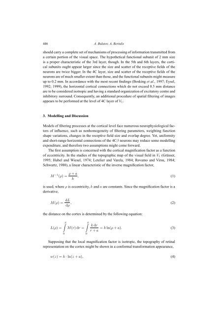
The first assumption is concerned with the cortical magnification factor as a function
of eccentricity. In the studies of the topographic map of the visual field in V 1 (Grüsser,
1995; Hubel and Wiesel, 1974; Letelier and Varela, 1984; Rovamo and Virsu, 1984;
Schwartz, 1980), a linear characteristic of the inverse magnification factor,
M −1 (ρ) = ρ + a
k , (1)
is used, where ρ is eccentricity, k and a are constants. Since the magnification factor is a
derivative,
M(ρ) = dL
dρ , (2)
the distance on the cortex is determined by the following equation:
L(ρ) =
∫ ρ
0
M(r)dr =
∫ ρ
0
k dr
= k ln(ρ + a). (3)
r + a
Supposing that the local magnification factor is isotropic, the topography of retinal
representation on the cortex might be shown in a conformal transformation appearance,
w(z) =k · ln(z + a), (4)