LINEAR AND CIRCULAR ARRAY OPTIMIZATION: A STUDY ... - PIER

360 Khodier and Al-Aqeel
Gain (dB)
0
-5
-10
-15
-20
-25
-30
-35
max(SLL) = -16.2037
PSO
Conv.
-40
0 20 40 60 80 100 120 140 160 180
Phase [deg]
350
300
250
200
150
100
2 4 6 8 10 12 14 16 18 20
Azimuth angle (deg)
Element #
(a) (b)
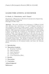
Figure 13. (a) Radiation pattern of 20-elements linear array
optimized with respect to phases ϕn’s to minimize the maximum SLL
and radiate towards φd = 45 ◦ with ∆φd = 22 ◦ . (b) The corresponding
element phases compared with λ/2 spaced conventional array steered
towards φd = 45 ◦ .
3. CIRCULAR ARRAY OPTIMIZATION
The PSO method is also employed to determine an optimum set of
weights and/or antenna element separations to create a non-uniform
circular isotropic array that maintains low side lobes. Also, dipole
circular arrays are widely used in communication systems as the
components for signal receiving [58]. Therefore, circular dipole array
are also considered here to determine the optimum set of excitations,
antenna elements separations and dipoles lengths.
3.1. Isotropic Circular Array
We consider isotropic circular array and optimize the radiation pattern
of the array in the term of the SLL reduction. The PSO algorithm
is used to determine the complex weights αn and/or the separation
between elements dmn where n = 1, . . . , N and N is the total number
of elements in the array. The array geometry is shown in Figure 14 for
an array of N elements. The array factor for such array is given in [59]
as:
AF (φ, α, dm) =
N�
n=1
50
0
j(ka cos(φ−φn))
αne
(9)
αn = Ine jϕn (10)