LINEAR AND CIRCULAR ARRAY OPTIMIZATION: A STUDY ... - PIER

Progress In Electromagnetics Research B, Vol. 15, 347–373, 2009 

LINEAR AND CIRCULAR ARRAY OPTIMIZATION: 

A STUDY USING PARTICLE SWARM INTELLIGENCE 

M. Khodier and M. Al-Aqeel 

Department of Electrical Engineering 

Jordan University of Science & Technology 

P. O. Box 3030, Irbid 22110, Jordan 

Abstract—Linear and circular arrays are optimized using the particle 

swarm optimization (PSO) method. Also, arrays of isotropic and 

cylindrical dipole elements are considered. The parameters of 

isotropic arrays are elements excitation amplitude, excitation phase 

and locations, while for dipole array the optimized parameters are 

elements excitation amplitude, excitation phase, location, and length. 

PSO is a high-performance stochastic evolutionary algorithm used 

to solve N-dimensional problems. The method of PSO is used to 

determine a set of parameters of antenna elements that provide the 

goal radiation pattern. The effectiveness of PSO for the design of 

antenna arrays is shown by means of numerical results. Comparison 

with other methods is made whenever possible. The results reveal that 

design of antenna arrays using the PSO method provides considerable 

enhancements compared with the uniform array and the synthesis 

obtained from other optimization techniques. 

1. INTRODUCTION 

The methods used for the synthesis of antenna arrays can be broadly 

classified into two categories: deterministic and stochastic. The 

deterministic methods include analytical methods [1–8] and semianalytical 

methods [9–15]. The deterministic methods in general 

become quite involved and computationally time consuming as the 

number of the elements in the array increases. 

On the other hand, stochastic methods are now very common 

in electromagnetics, and have many advantages over deterministic 

Corresponding author: M. Khodier (majidkh@just.edu.jo).

348 Khodier and Al-Aqeel 

methods [16]. These methods include neural networks (NN) [17– 

19] and evolutionary algorithms such: genetic algorithm (GA) [20– 

32], simulated annealing (SA) [33–36], differential evolution (DE) [37], 

and Tabu search (TS) [38]. The advantages of using stochastic 

methods are their ability in dealing with large number of optimization 

parameters, avoiding getting stuck in local minima, and relatively easy 

to implement on computers. Another recently invented evolutionary, 

high-performance algorithm is the particle swarm optimization (PSO) 

method introduced in [39, 40]. It requires fewer lines of code than GA 

or SA and easier to implement. Another advantage of PSO against GA 

is the small number of parameters to be tuned. In PSO, the population 

size, the inertial weight and the acceleration constants summarize the 

parameters to be scaled and tuned, whereas in GA the population size, 

the selection, crossover and mutation strategies, as well as the crossover 

and mutation rates influence the result [41]. Also, [41] shows that PSO 

algorithm convergence is faster than GA and SA for the same problem 

and the main computational time is lower than SA, binary GA, real 

GA, binary hybrid GA, and real hybrid GA. The literature on the 

use of the PSO method in the design of antenna arrays is extensive, a 

sample of which can be found in [42–57]. In this paper, the method of 

PSO is used to provide a comprehensive study of the design of linear 

and circular antenna arrays. The parameters of antenna elements 

that provide the goal radiation pattern are optimized using the PSO. 

The effectiveness of PSO for the design of antenna arrays is shown 

by means of numerical results. Comparison with other methods is 

made whenever possible. The results reveal that design of antenna 

arrays using the PSO method provides considerable enhancements 

compared with the uniform array and the synthesis obtained from other 

optimization techniques. 

2. LINEAR ANTENNA ARRAY 

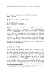
An 2N-element array distributed symmetrically along x-axis is 

considered as shown in Figure 1. The array factor is 

AF (φ) = 2 

N� 

In cos[kxn cos(φ) + ϕn] (1) 

n=1 

where k is the wavenumber, and In, ϕn and xn are, respectively, the 

excitation amplitude, phase, and location of element n. The element 

number 1 (n = 1) is placed at x1 = λ/4.

Progress In Electromagnetics Research B, Vol. 15, 2009 349 

Figure 1. Geometry of the 2N-element symmetric linear array placed 

along the x-axis. 

2.1. Minimize the Maximum SL Peak 

The PSO algorithm is used to obtain the optimum synthesis of a 

2N-element linear array in order to minimize the maximum SLL in 

a specific region. The fitness function is formulated as 

fitness = min (max {20 log |AF (φ)|}) 

2.1.1. Optimize Elements Amplitude In 

subject to φ ∈ {[0 ◦ , 76 ◦ ]&[104 ◦ , 180 ◦ ]} 

Here, we optimize In’s of the array and fix ϕn’s and xn’s. The fixed 

parameters are those of the uniform array, i.e., ϕn = 0 and the spacing 

between elements is λ/2, n = 1, . . . , N. The initial values of the 

amplitudes are set to be uniformly distributed from [0, 1]. The search 

region for each agent in the swarm is from [0, 1]. The normalized results 

from the optimization are given in Table 1. Also a Chebyshev array 

Table 1. 2N = 10 elements optimized using PSO with respect 

to amplitudes constraint compared with Chebyshev method with 

maximum SLL = −24.6217 dB (the values are normalized). 

Element 1 2 3 4 5 

�In� PSO 1.0000 0.9010 0.7255 0.5120 0.4088 

�In� Cheby. 1.0000 0.9010 0.7255 0.5119 0.4088 

(2)


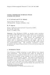
that results in the same SLL is shown in the same table. The amplitude 

distributions along the array elements are shown in Figure 2(b). The 

values of the amplitude are decreasing from the center of the array 

to the edges. The corresponding radiation pattern in the azimuth 

plane (x-y plane) compared with uniform array is shown in Figure 2(a). 

The maximum SLL obtained is −24.6217 dB while the maximum SLL 

of the uniform one is −13 dB. The proposed array SLL is less than 

the uniform one of about 11.6 dB. The smooth amplitude distribution 

makes it possible to use power dividers. However, from Figure 2(a) 

we note that the beamwidth of the optimized array is slightly larger 

than the conventional one since it is well known that the uniform 

array is optimum in terms of beamwidth. Nevertheless, the difference 

between the two is very small. Recently in [38], linear array’s element 

Gain (dB) 

0 

-5 

-10 

-15 

-20 

-25 

-30 

-35 

-40 

0 20 40 60 80 100 120 140 160 180 

0.4 

5' 4' 3' 2' 1' 1 2 3 4 5 

Azimuth angle (deg) Element # 

(a) 

PSO 

Conv. 

normalized amplitude 

Figure 2. (a) Radiation pattern of 10 elements λ/2 spaced array 

optimized with PSO with respect to amplitudes, compared with 

conventional array. (b) Normalized amplitude distribution �In� of 

array elements using PSO in Table 1. 

Table 2. 2N = 16 elements optimized using PSO with respect 

to amplitudes using (3) and (4) constraint compared with TSO and 

Chebyshev methods with maximum SLL = −30.7 dB (the values are 

normalized). 

Element 1 2 3 4 5 6 7 8 SLL [dB] 

In TS [38] 1.0000 0.9627 0.8766 0.7560 0.6105 0.4833 0.2957 0.3426 -30.4 

In PSO 1.0000 0.9521 0.8605 0.7372 0.5940 0.4465 0.3079 0.2724 -30.7 

In Cheby. 1.0000 0.9515 0.8602 0.7364 0.5933 0.4457 0.3069 0.2713 -30.7 

1.1 

1 

0.9 

0.8 

0.7 

0.6 

0.5 

(b)


amplitudes are optimized using the Tabu search optimization method 

(TSO) to minimize the maximum SLL. The results obtained from PSO 

versus TSO result are tabulated in Tables 2 and 3 for 16-element array 

and 24-element array, respectively. Also, values of Chebyshev array 

are given in the tables where the maximum SLL is the same from PSO 

method. 

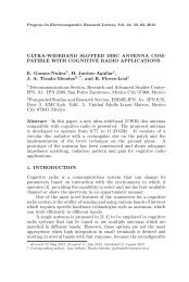
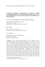
From Tables 1–3, we see that the PSO results are almost identical 

to Chebyshev one. Also, the maximum SLL obtained from PSO is 

less than the TSO method in all cases. In [38], a comparison is 

made between TSO and Chebyshev algorithm and the results are not 

identical. Figures 3 and 4 illustrate the array factor compared with 

conventional array, and the amplitude distribution of PSO compared 

with TSO in Tables 2 and 3. 

Table 3. 2N = 24 elements optimized using PSO with respect to 

amplitudes constraint compared with TSO and Chebyshev methods 

with maximum SLL = −34.5 dB (the values are normalized). 

Gain (dB) 

Optimization 

method 

�In� TS [38] 

�In� PSO 

�In� Cheby. 

0 

-5 

-10 

-15 

-20 

-25 

-30 

-35 

-40 

-45 

-50 

1.0000,0.9811,0.9373,0.8850,0.7883,0.7294, 

0.5984,0.5319,0.4051,0.3381,0.2123,0.3197 

1.0000,0.9712,0.9226,0.8591,0.7812,0.6807, 

0.5751,0.4768,0.3793,0.2878,0.2020,0.2167 

1.0000,0.9758,0.9289,0.8619,0.7787,0.6839, 

0.5824,0.4794,0.3795,0.2870,0.2049,0.2225 

PSO 

Conv. 

0 20 40 60 80 100 120140 160 180 


1.1 

1 

0.9 

0.8 

0.7 

0.6 

0.5 

0.4 

0.3 

SLL 

[dB] 

−33.0 

−34.5 

−34.5 

PSO 

TSO 

0.2 

8' 7' 6' 5' 4' 3' 2' 1' 1 2 3 4 5 6 7 8 

Element # 

Azimuth angle (deg) 

(a) (b) 

Figure 3. (a) Radiation pattern of 16 elements λ/2 spaced optimized 

using PSO with respect to amplitudes, compared with conventional 

array. (b) Normalized amplitude distribution.


Gain (dB) 

0 

-5 

-10 

-15 

-20 

-25 

-30 

-35 

-40 

-45 

PSO 

Conv. 

-50 

0 20 40 60 80 100 120 140 160 


(a) 


1.1 

1 

0.9 

0.8 

0.7 

0.6 

0.5 

0.4 

0.3 

PSO 

TSO 

0.2 

12'11'10' 9' 8' 7' 6' 5' 4' 3' 2' 1' 1 2 3 4 5 6 7 8 9101112 

Element # 

(b) 

Figure 4. (a) Radiation pattern of 24 elements λ/2 spaced optimized 

using PSO with respect to amplitudes, compared with conventional 

array. (b) Normalized amplitude distribution. 

Gain (dB) 

0 

-5 

-10 

-15 

-20 

-25 

-30 

-35 

PSO 

conv. 

-40 

0 20 40 60 80 100 120 140 160 180 


Figure 5. Radiation pattern 

of 10 elements λ/2 spaced, optimized 

with respect to phases compared 

with the uniform phases 

conventional case. 

2.1.2. Optimize Elements Phases ϕn 

Gain [dB] 

0 

-5 

-10 

-15 

-20 

-25 

-30 

-35 

PSO 

Conv . 

-40 

0 20 40 60 80 100 120 140 160 180 

Angle 

Figure 6. Radiation pattern of 

10-elements linear array positions 

optimized using (3) compared 

with the uniform case. 

We fixed In = 1 and the spaces between elements is λ/2 as the uniform 

array. The first element phase is fixed to ϕ1 = 0 ◦ . Initial phase values 

are uniformly distributed in [0, 180 ◦ ]. Table 4 shows the corresponding 

phases of the array. 

Figure 5 shows the radiation pattern of the array compared with 

uniform array and the maximum SLL is −24.62 dB which is higher 

than the case were the amplitudes are non-uniform of only 0.0017 dB, 

but still better than the uniform one in terms of SLL.


Table 4. 2N = 10 elements optimized with respect to phases. 

Element 1 2 3 4 5 

ϕn [deg] 00.0000 25.7120 43.4847 59.2084 64.8670 

Table 5. 2N = 10 elements optimized with respect to positions. 

Element 1 2 3 4 5 

±xn[λ] 0.2146 0.5999 1.0611 1.5870 2.2500 

The smooth phase distribution may allow using delay circuit to 

perform the needed phase shifts. 

2.1.3. Optimize Element Positions xn 

We fix the amplitudes and phases as the case of λ/2 spaced 

conventional array (In = 1 and ϕn = 0 ◦ ), and adjust the positions 

xn’s by the PSO. The total length of a 10-elements, λ/2 spaced 

uniform array is 4.5λ. Therefore, we fix the last elements positions 

to x±N = ±2.25λ, and the problem is solved in a four-dimensional 

solution space. The minimum distance between two neighboring 

elements is |xi − xj| = 0.25λ, where i = 1, 2, 3, 4 and i �= j. This 

leads to min(xi) = 0.125λ. 

The optimum element positions obtained from PSO are given in 

Table 5. The relative radiation pattern is shown in Figure 6 along with 

the λ/2 spaced conventional array pattern. It should be mentioned here 

that our results exactly matches the results in [45]. The maximum peak 

in the SLL region is about −19.7167 dB which is lower of about 6.7 dB 

from the uniform array. 

Some applications are interested in the minimizing the close-in 

SLL (the first sidelobe nearest to the main beam). To achieve this 

property, a modified fitness is used: 

fitness = min(α1 max {20 log |AF (φAS)|} 

+α2 max {20 log |AF (φNS)|}) (3) 

subject to φAS ∈ {[0 ◦ , 76 ◦ ]&[104 ◦ , 180 ◦ ]} 

and φNS ∈ {[69 ◦ , 76 ◦ ]&[104 ◦ , 111 ◦ ]} (4) 

This fitness function has an advantage of controlling the near sidelobe. 

The region specified by φAS is the same region as (2) and α1 is its 

weight. The close-in sidelobe region is specified by φNS and α2. This 

modification allows the near sidelobe region to be controlled and the 

amount of its reduction depends on the values of α1 and α2.


Angle 

Figure 7. Radiation pattern of 10 elements array positions optimized 

in Table 6 compared with the array in Table 5. 

Table 6. 2N = 10 elements optimized with respect to positions. 

Element 1 2 3 4 5 

±xn[λ] 0.1685 0.5461 0.9364 1.5107 2.25 

For example, a 10-element linear array is optimized using the 

fitness function given by (3) and weights α1 = 1 and α2 = 2. Table 6 

shows the array elements positions and Figure 7 shows the difference 

between radiation pattern of the modified array and the array in 

Table 5. 

Although the far sidelobe region is about −18.3 dB which is higher 

than the previous case of about 1.4 dB, the near sidelobe is minimized 

to −31 dB and the reduction is about 11.3 dB from the previous case 

and about 18 dB from λ/2 spaced uniform array. 

2.1.4. Optimize Array Amplitudes (In), Phases (ϕn) and Separations 

(xn) 

Here, all array parameters are optimized. The first element phase is set 

to zero as a reference to other elements. The initial elements positions 

are set as in the λ/2 spaced uniform array, and the edge elements are 

set to ±(N − 0.5)(λ/2) which is also used as the upper limit for the 

positions. The lower limit is defined as ±0.25(λ/2). So the positions 

searching region can be defined as 0.25λ/2 < xn < (N − 1/2)(λ/2) 

where n = 1, . . . , (N − 1).


Gain (dB) 

0 

-5 

-10 

-15 

-20 

-25 

-30 

-35 

PSO 

Conv . 

-40 

0 20 40 60 80 100 120 140 160 180 


Figure 8. Radiation pattern of 10-elements array positions optimized 

with respect to amplitudes (In), phases (φn) and separations (xn) 

compared with λ/2 spaced uniform array. 

Table 7. 2N = 10 elements optimized with respect amplitudes (In), 

phases (ϕn) and separations (xn) using (2). 

Element 1 2 3 4 5 

ϕn [deg] 0 40.49 54.24 49.46 51.97 

�In� 1.0000 0.82 0.94 0.96 0.72 

xn[λ] 0.28 0.77 1.10 1.61 2.25 

The PSO produced an array with parameters given in Table 7. 

The corresponding radiation pattern is shown in Figure 8 compared 

with λ/2 spaced conventional array. The maximum SLL here is 

−25.271 dB which is 12.271 dB lower than the λ/2 spaced conventional 

array, 0.644 dB lower than the arrays in Sections 2.1.1 and 2.1.2 and 

5.555 dB lower than the array in Section 2.1.3. The array parameters 

obtained are different than the parameters obtained in the previous 

three sections. Also, we can see from Table 7 that the current and 

phase distributions are not smooth like the results in Sections 2.1.1 

and 2.1.2. The enhancement here is good compared to the conventional 

and Section 2.1.3 arrays, but it is not much different from Sections 2.1.1 

and 2.1.2 arrays. 

2.2. Minimize the SL Average Power 

In this section, we are interested in the design of linear antenna array 

with minimum average SL power. To achieve this goal, the following


function is used to evaluate the fitness: 

⎛ 

⎜� 

� 

1 

fitness = min ⎝ 

∆φi 

i 

φui 

φli 

⎞ 

|AF (φ)| 2 ⎟ 

dφ⎠ 

(5) 

where [φli, φui] is the spatial regions in which the SLL is suppressed 

and ∆φi = φui − φli. The sidelobe regions are specified by 

φl1 = 0 ◦ , φu1 = 81 ◦ , φl2 = 99 ◦ , φu2 = 180 ◦ . (6) 

The integration in (5) doesn’t have a closed form and should be 

evaluated numerically. For this purpose, we use a 32 point Gaussian- 

Legender method. 

2.2.1. Optimize Element Amplitudes In 

The amplitudes are initialized randomly within the interval [0, 1] which 

also represents the searching region. Table 8 shows the corresponding 

amplitudes and Figure 11 shows the array radiation pattern compared 

with the pattern of conventional case. 

It can be seen from Figure 9 that the conventional array exhibits 

relatively high SLL, while the PSO algorithm offers an improvement in 

terms of SLL suppression. Table 8 shows that the element amplitudes 

are decreasing from the center of the array to the edges. 

Table 8. 2N = 10 elements optimized with respect to amplitudes 

using (5). 

Element 1 2 3 4 5 

�In� 1.000 0.8122 0.6799 0.5655 0.3546 

2.2.2. Optimize Element Phases ϕn 

Element amplitudes In’s and positions xn’s are fixed as the λ/2 spaced 

conventional array. As a reference, the first element phase is fixed 

to zero. The result found by the PSO algorithm is the same as the 

conventional array, i.e., ϕn = 0 ◦ for all n = 1, 2, . . . , N, and we can 

say that the λ/2 spaced conventional array is optimum in the sense of 

minimizing (5).


Gain (dB) 

0 

-10 

-20 

-30 

-40 

-50 

PSO 

Conv. 

-60 

0 20 40 60 80 100 120 140 160 180 



10 elements positions optimized 

with respect to amplitudes (In), 

and compared with conventional 

array. 

Gai n (dB) 

0 

-10 

-20 

-30 

-40 

-50 

PSO 

Conv. 

-60 

0 20 40 60 80 100 120 140 160 180 



10-element array optimized with 

respect to positions xn’s, compared 

with conventional array. 

Table 9. 2N = 10 array optimized with respect to element positions 

using (5). 

Element 1 2 3 4 5 

dn[λ] 0.2529 0.5558 1.0635 1.4990 2.1101 

2.2.3. Optimize Element Positions xn 

Here, we freed the total array length and did not fix it as in 

previous sections. Initial positions for the PSO are as the λ/2 spaced 

conventional array to speed the PSO convergence. The searching 

region is within the interval [0.125, (N/2) − 0.5] λ/2. The array 

geometry obtained from PSO is shown in Table 9 which exactly 

matches the result in [42]. It can be seen from the table that the array 

length obtained using the PSO algorithm is less than the conventional 

array. The radiation pattern in Figure 10 shows more enhancements 

compared to the conventional array. 

2.2.4. Optimize Element Amplitudes In, Phases ϕn and Separations 

xn 

Table 10 shows the PSO results for amplitudes In’s, phases ϕn’s and 

separations xn’s. The array aperture is larger than the conventional 

array and the array in Section 2.1.4. Amplitude distribution is not 

smooth as the array in Section 2.1.1. The phases of the array are


Table 10. 2N = 10 array optimized with respect to element 

amplitudes In’s, phases ϕn’s and separations xn’s. 

Element 1 2 3 4 5 

ϕn [deg] 0.000 0.000 0.000 0.000 0.000 

�In� 1.000 0.5507 0.2761 0.5933 0.2913 

xn[λ/2] 0.7356 2.2084 2.2151 3.6712 5.0000 

exactly like the phases of the array in Section 2.2.2, which is the same 

as λ/2 spaced conventional array. So by controlling only elements 

amplitude and position, we can achieve an array with more SLL average 

reduction. The corresponding radiation pattern compared with the 

conventional one is plotted in Figure 11. The enhancement in the 

SSL average is more than the arrays obtained in Sections 2.2.1, 2.2.2 

and 2.2.3. 

Gain (dB) 

0 

-10 

-20 

-30 

-40 

-50 

PSO 

Conv. 

-60 

0 20 40 60 80 100 120 140 160180 


Figure 11. Radiation pattern of 10 elements optimized with respect 

to amplitudes (In), phases (ϕn) and separations (xn) compared with 

λ/2 spaced uniform array. 

2.3. Linear Array Beam Steering 

This section illustrates the ability of PSO algorithm to perform linear 

array beam steering. Here, the SLL band is the regions beside the 

main beam in which its maximum occurred at the goal steering angle. 

Elements amplitude and position are fixed as those of the conventional 

array and only phases are optimized. The used array factor is 

AF (φ) = 

2N� 

n=2 

exp (j[nπ cos(φ) + ϕn]) + 1 (7)


In (7), we assume uniform amplitude and positions, while setting 

ϕ1 = 0 ◦ as a reference. The sidelobe region is defined as 

φSLL ∈ 

� � 

0 ◦ , 

� 

φd − ∆φd 

2 

� ◦� 

, 

�� 

φd + ∆φd 

2 

� ◦ 

, 180 ◦ 

� � 

where φd is the steering angle, and ∆φd is the band where φd is 

included. The result for 20-element array are shown in Table 11. The 

array factor is plotted in Figure 12(a) with λ/2 spaced conventional 

array steered towards the same angle pattern as in [5], respectively. 

Element phases are plotted in Figure 12(b). Another example for a 

20-element array with φd = 45 ◦ and ∆φd = 22 ◦ optimized to minimize 

the maximum SLL is shown in Figure 13. The SLL reduction in this 

case is considered only in the near SL region but the array SLL obtained 

is larger than the conventional array in far SL region. 

Table 11. 20-elements array optimized with respect to phases to 

radiate towards φd = 45 ◦ with ∆φd = 14 ◦ . 

Gain (dB) 

ϕn[deg] 

Uniform array 

0 

-5 

-10 

-15 

-20 

-25 

-30 

-35 

ϕn[deg] 

PSO array 

-40 

0 20 40 60 80 100 120 140 160 180 

000.0,232.7,105.4,338.2,210.9,083.6,316.3, 

189.0,061.8,294.5,167.2,039.9,272.6,145.4, 

018.1,250.8,123.5,356.3,229.0,101.7. 

0.000,253.0,134.0,006.5,237.9,109.7,343.3, 

217.1,091.3,324.8,197.8,070.9,304.9,179.0, 

051.8,284.6,156.1,028.8,268.8,165.9. 

PSO 

Conv. 

Phase [deg] 

350 

300 

250 

200 

150 

100 


Element # 

(a) (b) 

50 

0 

PSO 

Conv 

(8) 

2 4 6 8 10 12 14 16 18 20 

Figure 12. (a) Radiation pattern of 20-elements linear array 

optimized with respect to phases ϕn’s to radiate towards φd = 45 ◦ 

with ∆φd = 14 ◦ . (b) The corresponding element phases compared 

with λ/2 spaced conventional array steered towards φd = 45 ◦ .


Gain (dB) 

0 

-5 

-10 

-15 

-20 

-25 

-30 

-35 

max(SLL) = -16.2037 

PSO 

Conv. 

-40 

0 20 40 60 80 100 120 140 160 180 

Phase [deg] 

350 

300 

250 

200 

150 

100 

2 4 6 8 10 12 14 16 18 20 


Element # 

(a) (b) 

Figure 13. (a) Radiation pattern of 20-elements linear array 

optimized with respect to phases ϕn’s to minimize the maximum SLL 

and radiate towards φd = 45 ◦ with ∆φd = 22 ◦ . (b) The corresponding 

element phases compared with λ/2 spaced conventional array steered 

towards φd = 45 ◦ . 

3. CIRCULAR ARRAY OPTIMIZATION 

The PSO method is also employed to determine an optimum set of 

weights and/or antenna element separations to create a non-uniform 

circular isotropic array that maintains low side lobes. Also, dipole 

circular arrays are widely used in communication systems as the 

components for signal receiving [58]. Therefore, circular dipole array 

are also considered here to determine the optimum set of excitations, 

antenna elements separations and dipoles lengths. 

3.1. Isotropic Circular Array 

We consider isotropic circular array and optimize the radiation pattern 

of the array in the term of the SLL reduction. The PSO algorithm 

is used to determine the complex weights αn and/or the separation 

between elements dmn where n = 1, . . . , N and N is the total number 

of elements in the array. The array geometry is shown in Figure 14 for 

an array of N elements. The array factor for such array is given in [59] 

as: 

AF (φ, α, dm) = 

N� 

n=1 

50 

0 

j(ka cos(φ−φn)) 

αne 

(9) 

αn = Ine jϕn (10)


ka = 

N� 

dmi 

i=1 

φn = 2π 

n� 

� 

N� 

dmi dmi 

i=1 

i=1 

(11) 

(12) 

In, ϕn represents the amplitude and the phase excitation of the nth 

element in the array with respect, dmn represents the separation (arc 

longitude) from element n to element n + 1, k = 2π/λ the wave 

number, φ is the angle of incidence of a plane wave and λ is the 

signal wavelength. From the previous array factor we can formulate the 

objective function for the PSO to be optimized. Let AF (α, φmsl, dm) 

is the value of the array factor where the maximum sidelobe is attained 

at φmsl within the scanning ranges [0, φ1] and [φ2, 360]. The array will 

direct its main beam towards the angle φdis, and the fitness function 

is formulated as 

fitness = min(max(20 ∗ log(AF (α, φmsl, dm)/AF (α, φdis, dm))) 

Subject to dmn ≤ D (13) 

where D is the maximum arc separation between element n and 

element n + 1. The PSO algorithm is applied to optimize circular 

isotropic array of ten elements while the scanning range is set to 

dm 4 

dm 5 

I 4 

I 3 

dm 3 

dm 6 

y 

I 2 

dm 2 

dm N-1 

I 1 

I dm 

N-1 N 

Figure 14. Isotropic circular array geometry. 

I 5 

I 6 

φ 

φ 

1 

I N 

dm 1 

x


[0, 158] ◦ and [202, 360] ◦ . Table 12 shows the result obtained from PSO 

where D = 2λ and the result obtained from genetic algorithm (GA) 

in [59]. From Table 12 we see that the PSO maximum sidelobe is less 

than GA result of about 1.5 dB and 0.262 dB of [60] where the PSO 

with multi-objective fitness function is used to minimize the first null 

beamwidth (FNBW), the average SL power and the maximum SLL. 

The beamwidth is also narrower of about 1.44 ◦ compared to [59] and 

about 0.23 ◦ compared to [60]. The aperture reduction is about 0.07λ 

from [59] but it is larger than [60] of about 0.108λ. Figure 15(a) shows 

Gain [dB] 

0 

-5 

-10 

-15 

-20 

-25 

PSO 

Ga 

11 hbm 

Gain [dB] 

φ [deg.] 

φ [deg.] 

(a) (b) 

Our result 

[63] [63] re result 

-30 

-30 

-150 -100 -50 0 50 100 150 -150 -100 -50 0 50 100 150 

Figure 15. (a) Radiation pattern for circular isotropic array of 10 

elements optimized with respect to I, dm as in Table 12 compared 

with the result from GA in [59] and the uniform array for D = 2λ. (b) 

PSO result in (a) compared with [60] result. 

Table 12. N = 10 elements isotropic circular array optimized with 

respect to excitations amplitude and phase and elements separation in 

the range [0, 158] ◦ and [202, 360] ◦ . 

In 

Uniform array 

dm / λ 

GA 

[59] 

PSO 

[60] 

PSO 

(our work) 

n 

I 

n 

n 

dm / λ 

In 

dm / λ 

n 

In 

dm / λ 

n 

1, 1, 1, 1, 1, 1, 1, 1, 1, 1 

-5 0 

-10 

-15 

-20 

-25 

0.5, 0.5, 0.5, 0.5, 0.5, 0.5, 0.5, 0.5, 0.5, 0.5 

0.9545, 0.4283, 0.3392, 0.9074, 0.8086, 0.4533, 

0.5634, 0.6015, 0.7045, 0.5948 

0.3641, 0.4512, 0.2750, 1.6373, 0.6902, 0.9415, 

0.4657, 0.2898 ,0.6456, 0.3282 

1.0000, 0.7529, 0.7519, 1.0000, 0.5062, 1.0000, 

0.7501, 0.7524, 1.0000, 0.5067 

0.3170, 0.9654, 0.3859, 0.9654, 0.3185, 0.3164, 

0.9657, 0.3862, 0.9650, 0.3174 

0.7383, 0.8737, 0.5782, 1.000 0.7088, 1.000, 

0.5782, 0.8737 0.7383, 0.7179 

0.3243, 0.9747, 0.4124, 0.9369, 0.3571 

0.3572, 0.9369, 0.4124, 0.9747, 0.3243 

Max(SLL) = −3.6 dB 

Aperture = 5λ 

3 dB BW = 25.8 deg 

Max(SLL) = −11.03 dB 

Aperture = 6.08λ 

3 dB BW = 25.46 deg 

Max(SLL) = −12.307 dB 


3 dB BW = 24.34 deg 

Max(SLL) = −12.5687 dB 


3 dB BW = 24.02 deg


the PSO obtained radiation pattern, compared with GA result [59] and 

the uniform array. Figure 15(b) shows the obtained radiation pattern 

compared with the PSO result in [60]. It is clearly seen that the far 

SLL is larger than that in [60]. 

More enhancements can be obtained if the excitations phase ϕn is 

also optimized. The result is shown in Table 13 for the same case 

in Table 12. From Table 13, the enhancement appears clearly in 

SLL, aperture and 3 dB beamwidth. From Figure 16 we can see the 

difference between the two cases. Also, the obtained array has better 


respect to excitations amplitude and phase and elements separation in 

the range [0, 158] ◦ and [202, 260] ◦ . 

In 

dmn/λ 

ϕn 

0.2478 0.9149 0.8054 

0.5610 1.0000 0.5610 

0.8054 0.9149 0.2478 

0.8254 

0.5462 0.6220 0.7513 

0.4910 0.4859 0.4860 

0.4910 0.7513 0.6220 

0.5462 

−33.3758, 11.5900, 48.9874, 

32.5824, 0, 32.5824, 

48.9874, 11.5900, −33.3758, 

48.5313 

Max(SLL)=−15.2853 dB 

Aperture=5.7929λ 

3 dB BW=22.54deg 


respect to excitations amplitude and phase and to elements separation 

in the range [0, 158] ◦ and [202, 360] ◦ for D = λ/2. 

In 

dn/λ 

ϕn 

1.0000 0.9539 0.6929 

0.8307 0.5462 0.8307 

0.6929 0.9539 1.0000 0.6702 Max(SLL)=−11.8441 dB 

0.4986 0.4613 0.3180 


0.4906 0.4993 0.4940 


0.4906 0.3180 0.4613 0.4986 

0 36.2445 60.0777 

78.1235 −20.5532 78.1235 

60.0777 36.2445 0 94.2095


Gain [dB] 

0 

-5 

-10 

-15 

-20 

-25 

PSO PSO opt. opt. phases 

PSO no opt. phases 

-30 

-150 -100 -50 0 50 100 150 

[deg.] 

φ 

Figure 16. Radiation pattern for 

circular isotropic array of 10 elements 

optimized with respect to 

I, ϕ, dm as in Table 13 compared 

with the result of optimize I, dm 

for D = 2λ. 

Gain [dB] 

0 

-5 

-10 

-15 

-20 

-25 

-30 

D D D=0.5 = = 0.5 

0.5 λ 

D D D=2 = = 2 

2 λ 

-150 -100 -50 0 50 100 150 

Figure 17. Radiation pattern 

for circular isotropic array of 10 

elements optimized with respect 

to I, ϕ, dm for D = λ/2 as in 

Table 14 compared with the result 

of optimize I, ϕ, dm for D = 2λ. 

properties than one in [60]. 

From the above examples, we see that more enhancements could 

be achieved every time we include more array parameters in the PSO 

algorithm, but all the time we get a result for the array aperture more 

than the uniform one. To deal with this situation, we can limit the 

maximum separation D. Table 14 shows the results obtained when the 

separation is set to D = λ/2, where the aperture obtained is 4.53λ and 

the maximum SLL is −11.84 dB. The same thing can be said about the 

beamwidth which is 24.98 ◦ compared with 25.8 ◦ degree for the uniform 

case. Figure 17 shows the radiation pattern compared with the case 

when the separation limit is D = 2λ. The obtained radiation pattern 

has equal ripples in the sidelobe region. 

3.2. Circular Dipole Array Optimization 

In this section, we deal with the more practical case that the elements 

of the circular array are dipoles. In optimizing circular dipole array, 

the parameters to be controlled are elements excitation (amplitude 

and phase), elements separation, elements radii and elements lengths. 

The radiation pattern from the array is shaped by these parameters. 

Figure 18 shows the proposed circular dipole array geometry. Analysis 

of circular dipole array is the same as isotropic circular array but here 

the elements are dipoles. Mutual coupling between elements affects 

the array properties and there is no closed form of the array pattern. 

φ


x 

z 

. . . dm 3 dm2 

dm 1 

dm N 

Figure 18. Circular dipole array geometry. 

φ 

Numerical and approximate techniques are effectively used to obtain 

the array structure. The method of moments (MOM) is used to obtain 

the current distribution on the dipoles including mutual coupling 

effects. A common approximation is made by assuming that the 

current distribution along the dipole is sinusoidal (the current vanishes 

at the dipole terminals). This assumption becomes less accurate when 

the dipoles lengths are not a fraction of λ/2. So, we cannot use this 

assumption when the element lengths are optimized. We have to take 

into account that the elements lengths should be λ/2 if we want to 

use this assumption [61]. For a z-directed thin cylindrical antenna of 

length l and radius a, with a current distribution I(z) along its length, 

the Hallen’s integral equation is given by [61] 

µ 

4π 

�l/2 

−l/2 

L 1 

I(z ′ )G(z − z ′ )dz ′ = −jωµεEin(z) (14) 

where, µ the permeability of the material, ε the permittivity of the 

material, Ein the incident field, ω = 2πf and f the frequency, 

G(z − z ′ ) = e−jkR 

R , R = � (z − z ′ ) 2 + a 2 , and a is the dipole radius. 

The current I(z) vanishes at the antenna ends, that is, I(l/2) = 

I(−l/2) = 0. If we assume that the dipole is fed from a gap in its 

center then the incident field value is determined from the fed voltage; 

it is zero for parasitic elements and none zero for active elements. The 

dipole is sampled into elements along the z-axis. Then, by solving 

the integral equation in (14) a system of equations is obtained from 

which that current distribution can be determined. From the current 

y


distribution on the dipoles, the radiation pattern and the gain can be 

calculated. 

We use the PSO algorithm to optimize the dipole circular array 

with respect to some of its parameters. First we fix the dipoles 

Table 15. N = 10 elements dipole circular array optimized with 

respect to excitations amplitude and phase, and elements separation 

in the range [0, 158] ◦ and [202, 260] ◦ for D = 2λ. 

Ln/λ 

In 

ϕn 

dmn/λ 

0.5000 0.5000 0.5000 

0.5000 0.5000 0.5000 

0.5000 0.5000 0.5000 

0.5000 

1.0000 0.4265 0.7866 

0.4141 0.3571 0.4141 

0.7866 0.9066 1.0000 

0.4265 

5.5947 45.7218 20.2796 

−9.7969 −22.4059 −9.7969 

−38.8068 45.7218 5.5947 

20.2796 

0.5275 0.5265 0.6203 

0.5989 0.4630 0.4630 

0.5989 0.6203 0.5275 

Gain [dB] 

0.5265 

0 

-5 

-10 

-15 

-20 

-25 

-30 

-35 

-150 -100 -50 0 50 100 150 

φ [deg.] 

Max(SLL)=−17.3232 dB 



ϕ 

Opt. Opt. In, I n , l ln, n , dn, d n , Ln L n 

Opt. Opt. In, I n , ϕ l ln, n , dn d n 

Figure 19. Radiation pattern for circular dipole array of 10 elements 

optimized with respect to L, I, ϕ, dm as in Table 16 compared with the 

result of optimizing I, ϕ, dm as in Table 15.


Table 16. N = 10 elements dipole circular array optimized with 

respect to excitations amplitude and phase, elements separation and 

elements lengths in the range [0, 158] ◦ and [202, 260] ◦ for D = 2λ. 

Ln 

In 

ϕn 

dmn/λ 

0.5369 0.6094 0.5045 

0.3232 0.5352 0.3232 

0.5045 0.5364 0.5369 

0.6094 

0.7481 1.0000 0.7312 

0.5773 0.4411 0.5773 

0.7312 1.0000 0.6957 

0.7481 

−1.8166 −77.7446 55.3737 

−33.6932 −41.1082 −33.6932 

55.3737 −77.7446 −8.7745 

−1.8166 

0.4427 0.8849 0.1870 

0.8297 0.6344 0.6344 

0.8297 0.4427 0.8849 

0.1870 

Max(SLL)=−17.8819 dB 



lengths and diameters and let the PSO algorithm determine the best 

excitations and separations in order to minimize the following fitness 

function 

fitness = min(max(20 ∗ log(g(φmsl, α, dm)/g(φdis, α, dm))) (15) 

where g(φ, α, dm) is the gain towards the azimuth angle φ. The PSO 

algorithm is used to optimize a 10 elements circular dipole array where 

all array elements are fed at the center and all of them are centered 

along a circle on the x-y plane. The dipoles length is fixed to λ/2 

and the diameters of the dipoles are also fixed to 0.0067λ. The result 

obtained from PSO algorithm is tabulated in Table 15. 

Next, we optimize the same previous array with respect to 

excitation, separation and dipoles length. The result obtained is 

tabulated in Table 16. A plot of radiation pattern is shown in 

Figure 19 compared with the previous result. Results show that slight 

enhancement is achieved in the maximum SLL and the 3 dB BW by 

optimizing elements lengths.


4. CONCLUSIONS 

In this paper, different antenna array types are optimized using the 

PSO method. This paper illustrates how to model the design of 

non-uniform antenna arrays for single or multi objective optimization. 

The well-known method of PSO is proposed as the solution for these 

design problems. This method efficiently computes the design of 

several antenna arrays to generate a radiation pattern with desired 

properties. In the first part of the paper, we dealt with linear arrays. 

The optimization objectives were: first, minimize the maximum SLL 

by adjusting the excitation amplitudes, excitation phases or elements 

positions along the x-axis, and then adjust all the previous parameters 

simultaneously. The numerical results show that the PSO method 

produces minimum SLL compared with the uniform conventional array 

and the array obtained from the Tabu search optimization (TSO) 

method. Second, we minimized the close-in SLL while minimizing the 

maximum far SLL. Results show that considerable reduction in the 

close-in SLL is achieved. Third, PSO is used to minimize the average 

SL power by adjusting all possible array parameters individually and 

then all of them simultaneously. Results found from PSO show that 

the average SL power obtained is lower than the uniform conventional 

array one. Fourth, the array excitation phases are adjusted with 

PSO to perform beamsteering in certain direction. The PSO is 

also used to optimize elements locations, excitations amplitude and 

excitation phases of circular arrays. The results found show that 

the maximum SLL obtained is lower than the uniform conventional 

array and GA array, and the array beamwidth is thinner. For 

practical implementation of circular array, a circular dipole array is 

optimized to minimize the maximum SLL. The method of moments 

is used to determine the current distributions on the dipoles. The 

optimized parameters are elements excitation amplitude, excitation 

phases, locations and lengths. The results show that minimum SLL 

can be achieved by optimizing these parameters using the PSO method. 

REFERENCES 

1. Schelkunoff, S., “A mathematical theory of linear arrays,” Bell 

Systems Technology Journal, Vol. 22, No. 1, 80–107, 1943. 

2. Keizer, W. P., “Fast low-sidelobe synthesis for large planar array 

antennas utilizing successive fast fourier transform of the array 

factor,” IEEE Trans. on Antennas and Propagat., Vol. 55, No. 3, 

715–730, March 2007. 

3. Woodward, P. M. and J. P. Lawson, “The theoretical precision


with which an arbitrary radiation pattern may be obtained from 

a source of finite size,” Proc. IEEE, Vol. 95, No. 1, 120–126, 1948. 

4. Dolph, C., “A current distribution for broadside arrays which 

optimizes the relationship between beamwidth and side-lobe 

level,” Institute of Radio Engineers (IRE), Vol. 34, No. 6, 335– 

348, 1946. 

5. Balanis, C. A., Antenna Theory Analysis and Design, 2nd edition, 

John Wiley & Sons, 1997. 

6. Moffett, A. L., “Array factors with non uniform spacing 

parameters,” IRE Trans. on Antennas and Propagat., Vol. 10, 

131–136, 1962. 

7. Ishimaru, A. and Y. S. Chen, “Thinning and broadbanding 

antenna arrays by unequal spacings,” IEEE Trans. on Antennas 

and Propagat., Vol. 13, 34–42, 1965. 

8. Lo, Y. T. and S. W. Lee, “A study of space tapered arrays,” 

IEEE Trans. on Antennas and Propagat., Vol. 14, No. 1, 22–30, 

January 1966. 

9. Ma, X. and B. K. Chang, “Least square method for optimum 

thinned antenna arrays,” IEEE Antennas and Propagat. Society 

International Symposium, Vol. 4, No. 13, 2232–2235, July 1997. 

10. Ng, B. P., “Designing array patterns with optimum inter-element 

spacings and optimum weights using a computer-aided approach,” 

Int. J. Electron., Vol. 73, No. 3, 653–664, September 1992. 

11. Ng, B. P., M. H. Er, and C. A. Kot, “Linear array aperture 

synthesis with minimum sidelobe level and null control,” IEE 

Proc. — Microwave Antennas Propagat., Vol. 141, No. 3, 2674– 

2679, June 1994. 

12. Ng, B. P., “Array synthesis using a simple computer-aided 

approach,” Electron. Lett., Vol. 26, No. 5, 337–339, March 1990. 

13. Ismail, T. H. and M. M. Dawoud, “Null steering in phased arrays 

by controlling the element positions,” IEEE Trans. on Antennas 

and Propagat., Vol. 39, No. 11, 1561–1566, November 1991. 

14. Er, M. H., S. L. Sim, and S. N. Koh, “Application of 

constrained optimization techniques to array pattern synthesis,” 

Signal Process, Vol. 34, No. 3, 323–334, 1993. 

15. Steinberg, B. D., “Comparison between the peak sidelobe of 

random array and algorithmically designed aperiodic arrays,” 

IEEE Trans. on Antennas and Propagat., Vol. 21, 366–369, 1973. 

16. Rahmat-samii, Y. and C. G. Christodoulou, “Special issue on 

synthesis and optimization techniques in electromagnetics and 

antenna system design,” IEEE Trans. on Antennas and Propagat.,


Vol. 55, No. 3, 518–522, March 2007. 

17. Shavit, R. and I. Taig, “Array pattern synthesis using neural 

networks with mutual coupling effect,” IEE Proc. Microw. 

Antennas Propag., Vol. 152, No. 5, 354–358, October 2005. 

18. Guney, K. and N. A. Sarikaya, “Hybrid method based 

combining artifical neural network and fuzzy inference system for 

simultaneous computation of resonant frequencies of rectangular, 

circular, and triangular microstrip antennas,” IEEE Trans. on 

Antennas and Propagat., Vol. 55, No. 3, 659–668, March 2007. 

19. Ng, B. P., “Array synthesis using a simple computer-aided 

approach,” Electron. Lett., Vol. 26, No. 5, 337–339, March 1990. 

20. Goldberg, D. E., Genetic Algorithms in Search, Optimization and 

Machine Learning, Addison-Wesley Longman Publishing Co. Inc., 

Boston, MA, 1989. 

21. Tennant, A., M. M. Dawoud, and A. P. Anderson, “Array 

pattern nulling by element position perturbations using genetic 

algorithm,” IEEE Electronics Letters, Vol. 30, No. 3, 174–176, 

February 1994. 

22. Ares, F., S. R. Rengarajan, E. Villanueva, E. Skochinski, and 

F. Moreno, “Application of genetic algorithms and simulated 

annealing technique in optimizing the aperture distributions of 

antenna array patterns,” Electron. Lett., Vol. 32, No. 3, 148–149, 


23. Samii, Y. R. and E. Michielssen, Electromagnetic Optimization by 

Genetic Algorithms, John Wiley and Sons, 1999. 

24. Merino, A. R., R. L. Miranda, and J. L. Bonilla, “Optimization 

method based on genetic algorithms,” Apeiron, Vol. 12, No. 4, 

394–408, October 2005. 

25. Marcano, J. D. and F. Duran, “Synthesis of antenna arrays using 

genetic algorithms,” IEEE Antennas and Propagat. Magazine, 

Vol. 42, No. 3, 12–20, June 2000. 

26. Haupt, R. L., “Thinned arrays using genetic algorithms,” IEEE 

Trans. on Antennas and Propagat., Vol. 42, No. 7, 993–999, 

July 1994. 

27. Shimizu, M., “Determining the excitation coefficients of an array 

using genetic algorithms,” IEEE Antennas and Propagat. Society 

International Symposium, Vol. 1, No. 20–24, 530–533, June 1994. 

28. Yan, K. K. and Y. Lu, “Sidelobe reduction in array-pattern 

synthesis using genetic algorithm,” IEEE Trans. on Antennas and 

Propagat., Vol. 45, No. 7, 1117–1122, July 1997. 

29. Jones, E. A. and W. A. Joines, “Design of Yagi-Uda antennas


using genetic algorithms,” IEEE Trans. on Antennas and 

Propagat., Vol. 45, No. 9, 1386–1392, September 1997. 

30. Donelli, M., S. Caorsi, F. Denatala, M. Pastorino, and A. Massa, 

“Linear antenna synthesis with a hybrid gentic algorithm,” 

Progress In Electromagnetics Research, PIER 49, 1–22, 2004. 

31. Mohanty, G. K., A. Chakrobarty, and S. Das, “Phase only 

and amplitude phase synthesis of dual pattern linear antenna 

arrays using floating point genetic algorithms,” Progress In 

Electromagnetic Research, PIER 68, 247–259, 2007. 

32. Misra, I. S., R. S. Chakrobarty, and B. B. Mangaraj, “Design, 

analysis and optimization of V dipole and its three element Yagi- 

Uda array,” Progress In Electromagnetic Research, PIER 66, 137– 

156, 2006. 

33. Ferreira, J. A. and F. Ares, “Pattern synthesis of conformal arrays 

by the simulated annealing technique,” Electron. Lett., Vol. 33, 

No. 14, 1187–1189, July 3, 1997. 

34. Kirkpatrick, S., C. D. Gellatt, and M. P. Vecchi, “Optimization 

by simulated annealing,” Science, Vol. 220, No. 4598, 671–680, 

1983. 

35. Murino, V., A. Trucco, and C. S. Regazzoni, “Synthesis of 

unequally spaced arrays by simulated annealing,” IEEE Trans. 

on Signal Processing, Vol. 44, No. 1, 119–123, January 1996. 

36. Ares, F., S. R. Rengarajan, E. Villanueva, E. Skochinski, and 

F. Moreno, “Application of genetic algorithms and simulated 

annealing technique in optimizing the aperture distributions of 

antenna array patterns,” Electron. Lett., Vol. 32, No. 3, 148–149, 


37. Rocha-Alicano, C., D. Covarrubias-Rosales, C. Brizuela- 

Rodriguez, and M. Panduro-Mendoza, “Differential evolution algorithm 

applied to sidelobe level reduction on a planar array,” 

AEU International Journal of Electronic and Communications, 

Vol. 61, No. 5, 286–290, 2007. 

38. Merad, L., F. Bendimerad, and S. Meriah, “Design of 

linear antenna arrays for side lobe reduction using the tabu 

search method,” The International Arab Journal of Information 

Technology, Vol. 5, No. 3, 219–222, July 2008. 

39. Kennedy, J. and R. C. Eberhart, “Particle swarm optimization,” 

Proc. IEEE Int. Conf. Neural Networks, Vol. 1942–1948, 

Piscataway, NJ, 1995. 

40. Eberhart, R. C. and Y. Shi, “Particle swarm optimization: Developments, 

applications and resources,” Proc. Congr. Evolutionary


Computation, Vol. 1, 81–86, 2001. 

41. Perez, J. R. and J. Basterrechea, “Comparison of different heuristic 

optimization methods for nearfield antenna measurements,” 

IEEE Trans. on Antennas and Propagat., Vol. 55, No. 3, 549–555, 

March 2007. 

42. Khodier, M. M. and C. G. Christodoulou, “Linear array 

geometry synthesis with minimum sidelobe level and null control 

using particle swarm optimization,” IEEE Trans. on Antennas 

Propagat., Vol. 53, No. 8, 2674–2679, August 2005. 

43. Bataineh, M. H. and J. I. Ababneh, “Synthesis of a periodic 

linear phased antenna array using particle swarm optimization,” 

Electromagnetics, Vol. 26, No. 7, 531–541, October 2006. 

44. Boeringer, D. W. and D. H. Werner, “Particle swarm optimization 

versus genetic algorithms for phased array synthesis,” IEEE 

Trans. on Antennas and Propagat., Vol. 52, No. 3, 771–779, 

March 2004. 

45. Nanbo, J. and Y. Rahmat-Samii, “Advances in particle swarm 

optimization for antenna designs: Real-number, binary, singleobjective 

and multiobjective implementations,” IEEE Trans. on 


46. Dennis, G. and Y. Rahmat-Samii, “Particle swarm optimization 

for reconfigurable phase differentiated array design,” Microwave 

and Optical Technology Letters, Vol. 38, No. 3, 168–175, August 5, 

2003. 

47. Baskar, S., A. Alphones, P. N. Suganthan, and J. J. Liang, 

“Design of Yagi-Uda antennas using comprehensive learning 

particle swarm optimization,” IEE Proc. in Microw. Antennas 

Propagat., Vol. 152, No. 5, 340–346, October 2005. 

48. Huang, T. and A. S. Mohan, “A microparticle swarm optimizer 

for the reconstruction of microwave images,” IEEE Trans. on 


49. Mahmoud, K. R., M. E. El-Adawy, S. M. M. Ibrahem, 

R. Bansal, and S. H. Zainud-Deen, “Comparison between 

circular and hexagonal array geometries for smart antenna 

systems using particle swarm optimization algorithm,” Progress 

In Electromagnetic Research, PIER 72, 75–90, 2007. 

50. Baskar, S., A. Alphones, P. N. Suganthan, and J. J. Liang, “Design 

of Yagi-Uda antennas using comprehensive learning particle 

swarm optimization,” IEEE Microwave Antenna Propagat., 

Vol. 152, No. 5, 340–346, October 2005. 

51. Chen, T. B., Y. L. Dong, Y. C. Jiao, and F. S. Zhang, “Synthesis of


circular antenna array using crossed particle swarm optimization 

algorithm,” Journal of Electromagnetic Waves and Applications, 

Vol. 20, No. 13, 1785–1795, 2006. 

52. Ciuprina, G., D. Ioan, and I. Munteanu, “Use of intelligent 

particle swarm optimization in electromagnetics,” IEEE Trans. 

on Magnetics, Vol. 38, No. 2, 1037–1040, March 2002. 

53. Robinson, J. and Y. Rahmat-Samii, “Particle swarm optimization 

in electromagnetics,” IEEE Trans. on Antennas and Propagat., 

Vol. 52, No. 2, 397–407, February 2004. 

54. Ababneh, J., M. Khodier, and N. Dib, “Synthesis of interdigital 

capacitors based on particle swarm optimization and artificial 

neural networks,” International Journal of RF and Microwave 

Computer-aided Engineering, Vol. 16, No. 4, 322–330, February 

2006. 

55. Xu, S. and Y. Rahmat-Samii, “Boundary conditions in particle 

swarm optimization revisited,” IEEE Trans. on Antennas and 

Propagat., Vol. 55, No. 3, 760–765, March 2007. 

56. Alander, J. T., L. A. Zinchenko, and S. N. Sorokin, “Analysis 

of fitness landscape properties for evolutionary antenna design,” 

IEEE International Conference on Artificial Intelligent Systems, 

363–368, 2002. 

57. Lohn, J. D., W. F. Kraus, D. S. Linden, and S. P. Colornbano, 

“Evolutionary optimization of Yagi-Uda antennas,” International 

Conference on Evolvable Systems, 236–243, Tokyo, October 3–5, 

2001. 

58. King, R. W. P., “Supergain antennas and the yagi and circular 

arrays,” IEEE Trans. on Antennas and Propagat., Vol. 37, No. 2, 

178–186, February 1989. 

59. Panduro, M. A., A. L. Mendez, G. Romero, and R. F. Dominguez, 

“Design of non-uniform circular antenna arrays for side lobe 

reduction using the method of genetic algorithms,” Vehicular 

Technology Conference VTC, Vol. 6, 2696–2700, May 2006. 

60. Shihab, M., Y. Najjar, N. Dib, and M. Khodier, “Design 

of non-uniform circular antenna arrays using particle swarm 

optimization,” Journal of Electrical Engineering, Vol. 5, No. 4, 

216–220, 2008. 

61. Orfanidis, S. J., “Electromagnetic waves and antennas,” 

www.ece.rutgers.edu/orfanidi/ewa., 2003.

LINEAR AND CIRCULAR ARRAY OPTIMIZATION: A STUDY ... - PIER

Create successful ePaper yourself

Delete template?

Save as template?