2 The BESSY Raytrace Program RAY - Helmholtz-Zentrum Berlin

2 

The BESSY Raytrace Program RAY 

F. Schäfers 

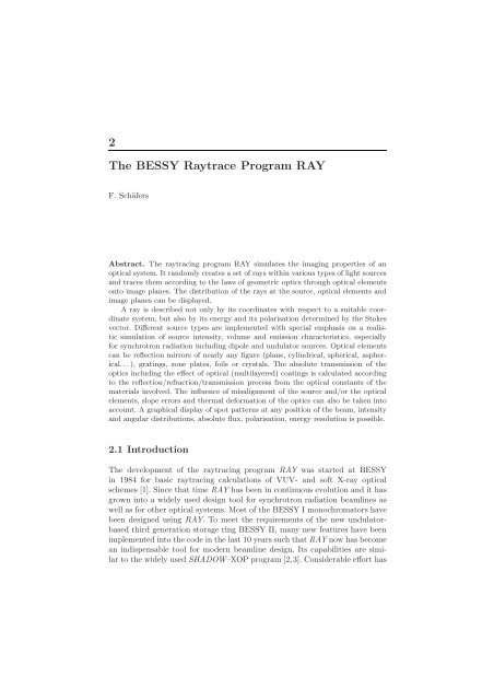
Abstract. The raytracing program RAY simulates the imaging properties of an 

optical system. It randomly creates a set of rays within various types of light sources 

and traces them according to the laws of geometric optics through optical elements 

onto image planes. The distribution of the rays at the source, optical elements and 

image planes can be displayed. 

A ray is described not only by its coordinates with respect to a suitable coordinate 

system, but also by its energy and its polarisation determined by the Stokes 

vector. Different source types are implemented with special emphasis on a realistic 

simulation of source intensity, volume and emission characteristics, especially 

for synchrotron radiation including dipole and undulator sources. Optical elements 

can be reflection mirrors of nearly any figure (plane, cylindrical, spherical, aspherical. 

. . ), gratings, zone plates, foils or crystals. The absolute transmission of the 

optics including the effect of optical (multilayered) coatings is calculated according 

to the reflection/refraction/transmission process from the optical constants of the 

materials involved. The influence of misalignment of the source and/or the optical 

elements, slope errors and thermal deformation of the optics can also be taken into 

account. A graphical display of spot patterns at any position of the beam, intensity 

and angular distributions, absolute flux, polarisation, energy resolution is possible. 

2.1 Introduction 

The development of the raytracing program RAY was started at BESSY 

in 1984 for basic raytracing calculations of VUV- and soft X-ray optical 

schemes [1]. Since that time RAY has been in continuous evolution and it has 

grown into a widely used design tool for synchrotron radiation beamlines as 

well as for other optical systems. Most of the BESSY I monochromators have 

been designed using RAY. To meet the requirements of the new undulatorbased 

third generation storage ring BESSY II, many new features have been 

implemented into the code in the last 10 years such that RAY now has become 

an indispensable tool for modern beamline design. Its capabilities are similar 

to the widely used SHADOW–XOP program [2,3]. Considerable effort has

10 F. Schäfers 

been made to ensure that it is a user friendly, easy accessable and easy-to-learn 

program for everyday use with a minimum effort on data and file handling. 

Alternative to these programs based on intensity distributions and geometric 

optics, wavefront propagation codes have been developed such as 

PHASE [4], which applies the Stationary Phase Approximation and SRW [5] 

employing Fourier Optics, which on the basis of the complex electric field 

of the radiation are able to intrinsically take into account interference and 

coherence effects. These codes are treated separately in this book [6]. 

This report is intended to be a practical reference and to give an outline 

of the underlying geometrical, mathematical, physical and optical principles 

which can be found in textbooks [7–9] or synchrotron radiation handbooks 

[10]. In particular, Chap. 3.2 of [10] (Ray tracing) is strongly recommended 

as an introductory guide before calculating a real beamline design. Here the 

procedure, problems, limitations and the importance of checking the raytrace 

results for the various kinds of errors that can occur are discussed. Various 

specific RAY-features have been described previously: crystal optics in [11] 

and zoneplate optics employing Fresnel diffraction where the collective effects 

are treated on a statistical (Monte Carlo) basis [12, 13]. Extended manuals 

for RAY [14] and the reflectivity program REFLEC [15] which share the 

same optics software library are also available. Examples for the use of the 

program in a variety of synchrotron radiation applications are given in [16]: 

plane grating monochromator (PGM-) beamlines, [17] IR-beamlines, [18] elliptical 

undulator beamlines, [19] gradient crystal monochromators, [20] μ-focus 

X-ray beamline. 

Chapter 3 explains the basic statistical treatment to simulate any kind 

of intensity patterns, while the next chapters describe the simulation of 

sources (Chap. 4), optical elements (Chap. 5) and of the treatment of absolute 

reflectivity and polarisation (Chap. 6). 

In Chap. 7 crystal diffraction optics employing dynamical theory is 

described. Looking ahead, in ‘Outlook’, the time evolution of the rays to 

describe wave, coherence and interference phenomena is discussed (Chap. 8). 

This extension of the program and the implementation of the zoneplate 

optics [12, 13] have been made possible by support through the COST-P7 

action and intensive discussions during the COST meetings. 

The complete code is available as a PC-Windows version. 

2.2 Beamline Design and Modelling 

The raytracing program RAY simulates the imaging and focussing properties 

of an optical system. It randomly creates a set of rays within various types of 

light sources and traces them through one or more optical elements on image 

planes. The geometric distribution of the rays at the source, at all optical 

elements and at the image planes can be visualized.

FEM 

ANSYS / ProE 

temperature distribution 

2 

photons/s/mm /BW 

x 10 

1000 

12 

800 

600 

400 

200 

vert. position (mm) 

2 The BESSY Raytrace Program RAY 11 

photon source 

WAVE / URGENT / SMUT 

JOB 38 UE52 

spatial distribution 

optical elements 

REFLEC 

E = 396eV 

1 

0.75 

0.5 

0.25 

1.5 

1 

0 

0.5 

-0.25 

0 

-0.5 

-0.5 

-0.75 -1 

-1.5 

-1 

Distribution in pinhole 

hori. position (mm) 

raytracing 

RAY 

blaze angle(°) 

1.0 

0.8 

0.6 

0.4 

0.2 

0.2 0.4 0.6 0.8 

cff 0.6 

0.4 

0.2 

0.0 

grating efficiency 

grating efficiency 

gratings 

EFFI 

y (mm) 

Intensity 

0.1 

0.0 

-0.1 

4000 

2000 

-0.05 0.00 0.05 0.10 

Width(x): 0.0472 mm 

Center : 0.014 mm 

0 

-0.05 0.00 0.05 0.10 

x (mm) 

Width(y): 0.0819 mm 

Center : -0.002 mm 

0.1 

0.0 

-0.1 

0 5000 

Intensity 

u41-162-0p7-40-ray 

1. image at : 755.00 mm 

N/s/0.1A/ 0.0mrad/ 0.1000%BW .1360D+16 

Transmission: 44.889 % 

112222( 112222) out of 250000 

N max /mm 2 : 0.6915D+18 

S1: 1.000 S2: 0.000 S3: 0.000 

spot pattern 

Fig. 2.1. BESSY soft X-ray computational tools and their interplay 

Various interesting features like focal properties, power distribution, energy 

resolution, rocking curves, absolute transmission and polarisation characteristics 

of an optical setup are simulated. It combines pure geometrical raytracing 

with calculations of the absolute transmission and is, thus, a central and 

indispensable part of the BESSY software tools for the design and optimization 

of new monochromators and beamlines from the infrared spectral 

region to the hard X-ray range. The interplay of the software tools available 

at BESSY [21, 22], is demonstrated in Fig. 2.1 as a flowchart. 

Special emphasis was put on realistic simulations of beamlines, in particular 

those employing synchrotron radiation: the path of the photons can be 

followed from any source, including bending magnets and insertion devices 

via reflection/diffraction/transmission at optical elements through apertures, 

entrance and/or exit slits on the sample. The influence of slope errors, surface 

roughness, thermal bumps, measured or calculated surface profiles as well as 

a misalignment of the source and optical elements can be studied in a simple 

way. Thus, it is possible to predict the real performance of the beamline under 

realistic conditions and to specify the requirements for all the components to 

be ordered. 

In a well defined source volume, rays are created within a given horizontal 

and vertical divergence. Each ray has the same intrinsic probability. 

The spatial and angular intensity distribution of the source is given by the 

spatial and angular density of the rays (i.e. rays per volume and solid angle). 

Thus, the outgoing rays simulate the intensity distribution of the corresponding 

source. The rays are traced according to geometrical optics through one 

or more optical elements (mirrors, gratings, foils, crystals, slits, zoneplates)


of which the surface can have nearly any figure such as plane, cylindrical, 

spherical, toroidal, paraboloidal or ellipsoidal and can be arranged in any 

geometry (horizontal, vertical, oblique). The absolute transmission of the 

optics including the effect of (multilayer-) coatings is calculated according 

to the reflection/refraction/transmission/diffraction processes from the optical 

constants of the involved materials. Special monochromator mounts and 

(coma-corrected) varied line-spacing (VLS-) gratings and (graded) crystals 

with automatic calculation of structure factors can also be handled. 

A ray is determined not only by its coordinates with respect to a suitable 

coordinate system (e.g. by its starting point) and by its direction, 

but also by its energy E, its polarisation, described by the Stokes vector 

S =(S0,S1,S2,S3), and its pathlength. Thus, a ray is described by 12 parameters, 

which are traced through the optical setup and for which the geometrical 

and optical modifications are calculated according to its interaction with the 

optical coating (reflection/refraction/transmission). Since all rays have equal 

probability (the intensity of a ray, S0, is either 1 or 0), the throughput of 

a beamline is simply given by the number of rays, for SR-sources multiplied 

with the absolute photon flux as scaling factor. 

For a first overview of the focal properties of an optical system, the horizontal 

and vertical widths of the beam can be visualized along the beam path 

for the determination of the focus position. At any position along the beam 

path image planes can be defined. The footprints of the rays on the optical 

elements and the focal properties of the optical system are analyzed and are 

visualized graphically as point diagrams, 2D or 3D intensity distributions etc. 

The menu-driven program is user friendly and so a first-performance test 

of an optical design can be gained rapidly without any file handling. Once the 

beamline has been defined the parameters are stored and can be modified in a 

subsequent run. The graphics output is directed to monitors, printers, or PS 

or EPS-files, and alternatively ASCII-data tables of all results can be created 

for further data evaluation and display. 

A flowchart of the program is shown in Fig. 2.2. 

2.3 Statistics: Basic Laws of RAY 

2.3.1 All Rays have Equal Probability 

To simulate realistic intensity patterns on optical elements and image planes 

(e.g. for heat load studies) it is necessary to create the source points and the 

rays in such a way that the same intensity is attributed to each ray. 

Generally there are two possibilities: 

• A systematic distribution of the rays within the source so that the real 

emission characteristic is simulated. For this a large number of rays is 

required and needs to be calculated before an optical setup is completely 

described.


Fig. 2.2. Flow chart of RAY 

• The rays are distributed statistically within the source so that within the 

statistical error the real emission characteristic is simulated. The intensity 

distribution of the source is thus understood as the probability distribution 

of the necessary parameters, namely position and angle. The main advantages 

of this Monto–Carlo procedure are its simplicity and the fact that a 

calculation of relatively few rays already is enough to create a reasonable


simulation of the optics. When the statistics and the accuracy seem to 

be sufficient, the calculation can always be interrupted without making a 

systematic error. 

This second option is realized in RAY. The procedure is as follows: 

1. Create a random number ran1 between 0 and 1. 

2. Scale the corresponding variable, e.g. the x-coordinate of the source point: 

x =(ran1 − 0.5) dx, (2.1) 

where dx is the source-dimension in the x-direction. 

3. Calculate the probability, w, of this randomly chosen start value for x (normalized 

to a maximum value of 1), for example the electron density in a 

dipole-source (gaussian profile w(x) =exp(−x2 /(2σ2 y)) or the synchrotron 

radiation intensity for a fixed wavelength at a definite horizontal and 

vertical emission angle (Schwinger theory [23]). 

4. Create a second random number ran2. The ray is accepted only if the 

difference of the probability w(x) and this new random number is larger 

than zero: 

w (x) − ran2 > 0. (2.2) 

5. If the difference is less than zero neglect this ray and start again with a 

new one according to (2.1). 

2.3.2 All Rays are Independent, but... (Particles and Waves) 

All rays are independent, and so they are considered as individual particles 

not knowing anything about each other. Thus, RAY works exclusively in the 

particle model. Nevertheless, the statistical method explained above is an 

elegant way to overcome the particle–wave dualism and to simulate wave 

phenomena and collective effects such as interference, diffraction, coherence 

and wave fronts. 

This is done by a statistical treatment of an ensemble of individual rays 

which behave within the statistical errors as a collective unit, as a wavefront. 

This random selection of a parameter is used extensively throughout the 

program not only to simulate the emission characteristics of a light source, 

but also, for example, to simulate the reflection angle on a mirror to simulate 

slope errors that are assumed to be gaussian. It is used to simulate reflection 

lossesofrayswherew(x) =R with (0

2.4 Treatment of Light Sources 


Various light sources are incorporated in RAY. Generally the rays are starting 

in a defined source volume and are emitted with a defined horizontal and 

vertical divergence. Either hard (flat-top) edges or a gaussian distribution 

profile can be simulated. In the latter case, rays are created statistically (see 

3.1) within a ±3σ-width of the gaussian profile (i.e. more than 99.9% of the 

intensity). 

For synchrotron radiation beamlines, the polarised emission characteristic 

of bending magnets, wigglers and undulators is incorporated. For other 

sources, such as twin or helical undulators, or to take beam emittance effects 

into account, the input can be given as an ASCII-file taken from programs 

for undulator radiation: URGENT [24], SMUT [25] or WAVE [26]. In this file 

the intensity and polarisation patterns of the light source must be described 

as intensity (photons/seconds) and Stokes parameters at a distance of 10 m 

from the centre of the source in a suitable x-y mesh. 

Each ray is attributed an energy, E, and a polarisation. The energy can be 

varied continuously within a ‘white’ hard-edge band of E0 ± ΔE, or toggled 

between three discrete energies E0, E0+ΔE and E0−ΔE. This feature allows 

one to determine easily the energy dispersion and the spatial separation of 

discrete energies for monochromator systems, thereby giving a picture of the 

energy resolution that one can expect. 

Table 2.1 lists the main features of the different light sources. 

The source coordinate system for the case of bending magnet synchrotron 

radiation is given in Fig. 2.3. The storage ring is located in the x-z plane, 

Table 2.1. Parameters of the RAY-sources 

Name Width Height Length Div. Div. S0 S1,S2,S3 

x y z hor. φ vert. ψ 

Matrix MA Hard Hard Hard Hard Hard 1 Input 

Point PO Hard Hard Hard Hard Hard 1 Input 

soft soft soft soft 

Circle CI Hard Hard Hard Hard Hard 1 Input 

Dipole DI Soft Soft Hard Hard Calc. Flux Calc. 

Wiggler WI Soft Soft L = nλu Hard Calc. Flux Calc. 

Wiggler/Undul. WU Soft Soft 0 Calc. Calc. Flux Input 

Double–Undul. HU Soft Soft Hard Soft Soft Flux Input 

Undul.–data file UF Soft Soft Hard File File Flux File 

Helical Undul. 

data file 

HF Soft Soft Hard File File Flux File 

Source data file FI Soft Soft Hard File File 1 Input 

hrd, a hard (flat-top) edge; soft, soft – a gaussian distribution of the respective 

variable within a 6σ-width is simulated; calc, calculated according to a theoretical 

model (e.g. Schwinger theory); n, number of wiggler periods; L, length of undulator; 

λu, period length; file, parameters taken from data-file; input, parameters to be given 

interactively


X so 

counter-clockwise rev. 

(e.g. BESSY I) 

Y so 

clockwise rev. 

(e.g. BESSY II) 

Fig. 2.3. Coordinate system for storage ring-bending magnet sources (DI pole) as 

viewed from above 

PO_int 

Z so 

PI_xel CI_rcle 

Fig. 2.4. Spot pattern of various source types in x-y plane, projected onto z =0 

DI_pole, 

Clockwise 

revolution 

DI_pole, 

Counter-Clockwise 

revolution 

WI_ggler, seen 

from top 

(x-z plane) 

Fig. 2.5. Spot pattern of synchrotron radiation sources in x-y plane, projected onto 

z =0 

for clockwise revolution of the electrons the x-axis is pointing away from the 

centre, while for counter-clockwise revolution the x-axis is pointing inside 

the storage ring centre. This is important to be noticed especially for optical 

systems with large horizontal divergence (e.g. IR-beamlines), where the 

source cross section is very asymmetric because of the depth-of-field effect 

(see Fig. 2.5). 

Examples of the intensity distribution (footprints) of various sources are 

given in the Figs. 2.4 and 2.5.


2.5 Interaction of Rays with Optical Elements 

2.5.1 Coordinate Systems 

The definition of the coordinate system used in RAY is shown in Figs. 2.6 

and 2.7. Its origin lies in the centre of the source (with the x-axis in general 

(e.g. SR) being horizontal). The coordinate system is transformed along the 

optical path from the source to the optical elements and then to the image 

planes. The z-axis points into the direction of the central ray, the x-axis 

is perpendicular to the plane of reflection, i.e. horizontal in the case of a 

vertically deviating optical setup (azimuthal angles 0 ◦ or 180 ◦ ), and it is 

vertical for horizontal mounts (azimuthal angles 90 ◦ (to the right) and 270 ◦ 

(to the left), respectively). The y-axis is always the normal in the centre of the 

optical element. The plane of reflection or dispersion is, thus, always the y-z 

plane and the surface of the optical elements is the x-z-plane, regardless of 

the azimuthal angle χ chosen. After the optical element the coordinate system 

X so 

ψ 

X so 

ψ 

φ 

Y so 

SOURCE 

φ 

COORDINATE SYSTEM OF RAY 

Vertical mount 

Y so 

χ 

χ 

Z so 

Z so 

α β 

YMi 2Θ 

XMi 1. OPTICAL 

ELEMENT 

X Mi 

α 

2Θ 

β 

Y Mi 

x Im 

Z Mi 

Horizontal mount 

y Im 

Z Mi 

z Im 

IMAGE 

PLANE 

Fig. 2.6. Coordinate system (right-handed screw) and angles used in RAY. (Top) 

Vertical deviation (upwards (downwards)) mount (azimuthal angle χ =0 ◦ (180 ◦ )). 

(Bottom) Horizontal deviation (to the right (left)) (azimuthal angle χ =90 ◦ (270 ◦ )). 

The optical element is always in the XM-ZM-plane 

Y Im 

χ 

X Im 

Z Im


x 

y 

z 

Fig. 2.7. Coordinate systems used in RAY. For optical elements (left) the coordinate 

system is fixed to the optical surface (X-Z plane). Transmission elements, screens 

and image planes (right) areintheX-Y plane, the x-axis is in the horizontal plane. 

The red line is the light beam 

for the outgoing ray is rotated back by −χ, i.e. it has the same orientation as 

before the optical element. In this way another optical element can be treated 

in an identical manner. 

2.5.2 Geometrical Treatment of Rays 

The geometric calculations proceed in the following way: 

Statistical creation of a ray within a given source volume and emission cone 

and within the ‘correct’ statistics (see Chap. 3). The ray is determined by its 

source coordinates (xs,ys,zs) and its direction cosines (ls,ms,ns) determined 

by the horizontal and vertical emission angles ϕ and ψ (see Fig. 2.8): 

⎛ 

�αS = ⎝ lS 

⎞ ⎛ ⎞ 

sin ϕ cos ψ 

mS ⎠ = ⎝ sin ψ ⎠ (2.3) 

cos ϕ cos ψ 

nS 

The vector equation of the ray is then 

or, in coordinates 

or 

�x = �xS + t�αS with tεℜ + 0 (2.4) 

⎛ 

⎝ x 

⎞ ⎛ 

y ⎠ = 

z 

x − xs 

lS 

⎝ xs 

ys 

= y − ys 

zs 

⎞ ⎛ 

⎠ + t 

mS 

= z − zs 

⎝ lS 

mS 

nS 

nS 

x 

y 

⎞ 

⎠ (2.5) 

z 

(2.6)

Y 

X 


x 

ψ 

ϕ 

n=cosϕcosψ 

m=sinψ 

l=sinϕcosψ 

Fig. 2.8. Source coordinate system: Definition of angles and direction cosines 

in RAY 

2.5.3 Intersection with Optical Elements 

The source coordinate is translated into a new coordinate system with the 

origin in the centre of the first optical element (hit by the central ray), and 

the z-axis parallel to a symmetry axis of the optical element (for a simplified 

equation). The coordinate system is translated by the ‘distance from the 

source’ totheopticalelement,zq, rotated around z by the azimuthal angle, 

χ, and around the new ˜x-axis by the grazing incidence angle, θ. Thetransformation 

to the new-coordinate system is performed by the following matrix 

operations: 

�xS ′ = D˜x (θ) Dz (χ) Tz (zq) �xS (2.7) 

zq distance source to first optical element or nth to (n + 1)th element 

θ rotation angle around x (y-z plane) 

χ azimuthal rotation around z (x-y plane) (clockwise), 

which corresponds to 

⎛ 

xS ′ 

⎝ yS ′ 

zS ′ 

⎞ ⎛ 

⎞ ⎛ 

⎞ ⎛⎛ 

1 0 0 cos χ −sinχ 0 

⎠ = ⎝0cosθ−sinθ⎠ ◦ ⎝sin χ cos χ 0⎠ 

◦ ⎝⎝ 

0sinθcos θ 0 0 1 

xS 

⎞ ⎛ 

yS ⎠ − ⎝ 

zS 

0 

0 

⎞⎞ 

⎠⎠ 

zq 

⎛ 

xS ′ 

or finally ⎝ yS 

(2.8) 

′ 

zS ′ 

⎞ ⎛ 

⎠ = ⎝ xs 

⎞ 

cos χ − ys sin χ 

xs sin χ cos θ + ys cos χ cos θ − (zs − zq)sinθ⎠ 

(2.9) 

xs sin χ sin θ + ys cos χ sin θ +(zs − zq)cosθ 

Z


The direction cosines are transformed correspondingly: 

and finally 

⎛ 

⎝ 

lS ′ 

mS ′ 

nS ′ 

�αS ′ = D˜x (θ) Dz (χ) �αS, (2.10) 

⎞ ⎛ 

⎠ = ⎝ ls 

⎞ 

cos χ − ms sin χ 

ls sin χ cos θ + ms cos χ cos θ ⎠ . (2.11) 

ls sin χ sin θ + ms cos χ sin θ 

In the new coordinate system the ray is described by 

⎛ 

⎝ x 

⎞ ⎛ 

xS ′ 

y ⎠ (t) = ⎝ yS 

z 

′ 

zS ′ 

⎞ ⎛ 

lS ′ 

⎠ + t ⎝ mS ′ 

nS ′ 

⎞ 

⎠ (2.12) 

2.5.4 Misalignment 

A six-dimensional misalignment of an optical element can be taken into 

account: three translations of the coordinate system by δx, δy and δz and 

three rotations by the misorientation angles δχ (x-y plane), δϕ (x-z plane) 

and δψ (y-z plane). Since the rotations are not commutative, the coordinate 

system is first rotated by these angles in the given order and then translated. 

For the outgoing ray to be described in the non-misaligned system, the coordinate 

system is backtransformed (in reverse order). Thus, the optical axis 

remains unaffected by the misalignment. 

2.5.5 Second-Order Surfaces 

Optical elements are described by the general equation for second-order 

surfaces: 

F (x, y, z) =a11x 2 + a22y 2 + a33z 2 +2a12xy +2a13xz 

+2a23yz +2a14x +2a24y +2a34z + a44 =0. 

(2.13) 

This description refers to a right-handed coordinate system attached to the 

centre of the mirror with its surface in x-z plane, and y-axis points to the 

normal). This coordinate system is used for the optical elements PL ane, 

CO ne, CY linder and SP here. 

Note that for the elements EL lipsoid and PA raboloid acoordinatesystem 

is used, which again is attached to the centre of the mirror (with x-axis on the 

surface), but the z-axis is parallel to the symmetry axis of this element for an 

easier description in terms of the aij parameters (see Figs. 2.9 and 2.10). The 

aij-values of Table 2.2 are given for this system. Thus, the rotation angle of 

the coordinate system from source to element is here θ +α (EL)and2θ (PA), 

respectively, θ being the grazing incidence angle and α the tangent angle on 

the ellipse.

Source 

Y So 

Z Y 

So Ell 

YMi Θ 

X So 

α 

Z o 

α 


Z Ell 

Z Mi 

Y Ell 

b 

Y o 

X Ell 

a 

Y Im 

Focus 

Fig. 2.9. Ellipsoid: definitions and coordinate systems 

Y Pa 

Directrix 

P 

Z o 

X Pa 

Y So 

θ 

X So 

Z Y 

So 

Pa 

YMi θ 

θ 

Z Pa 

Source 

Z Mi 

Fig. 2.10. Paraboloid: Definitions and coordinate systems 

Y Im 

X Im 

Z Im 

X Im 

Z Im 

The individual surfaces are described by the following equations: 

• Plane y =0 

• Cylinder(in z − dir.) x 2 + y 2 =0 

• Cylinder(in x − dir.) y 2 + z 2 =0 

• Sphere x 2 +(y − R) 2 + z 2 − R 2 =0 

• Ellipsoid x 2 /C 2 +(y − y0) 2 /B 2 +(z − z0) 2 /A 2 − 1=0 

• Paraboloid x 2 /C 2 +(y − y0) 2 /B 2 − 2P (z − z0) =0 

Z Pa 

Z Ell 

(2.14) 

Alternatively to the input of suitable parameters, such as mirror radii or 

half axes of ellipses, in an experts modus (EO), the aij parameters can be 

directly given, such that any second-order surface, whatever shape it has, can 

be simulated.


Table 2.2. Parameters of the second-order optical elements 

Name PM CY CO SP EL PA 

a11 0 1/0 1 − cm 1 B 2 /C 2 

P 2 /C 2 

a22 0 1 1 − 2cm 1 1 1 

a33 0 0/1 0 1 B 2 /A 2 

0 

a12 0 0 0 0 0 0 

a13 0 0 0 0 0 0 

� 

a23 0 0 

cm − c2 m 0 0 0 

a14 0 0 0 0 0 

a24 −1 ρ · sign −a23 R 

√ − R · sign −y0 −y0 

cm 

zm 

2 

a34 0 0 0 z0B 2 /A 2 

−P 

a44 0 0 0 0 y 2 0 + z2 0B2 /A 2 − B 2 

y 2 2 

0 − 2Pz0 − P 

Sign 

0 1/−1 1/−1 1/−1 1 1 

(concave/convex) 

Fx − (a11x + a12y + 0 −x/0 −x −a11x −a11x 

a13z + a14) 

Fy − (a22y · sign + 1 ρ · sign R · sign y0 − y y0−y a12x a23z + a24) 

Fz − (a33z + a13x + 0 0/−z −z −(z0 + z)(B/A) 

a23y + a34) 

2 

P 

z0 = A 2 /B 2 y0 tan(α) z0 = f cos(α, β) · sig 

y0 = ra sin(θ − α) y0 = f sin(2 α, β) 

tan(α) =tan(θ) P =2fsin 2 (θ)sig 

(ra − rb)/(ra + rb) 

ρ: radiusR, ρ: radii R: radius f: mirror–source/focus–dist. 

zm: mirror 

A, B, C half axes in z,y,x-dir; C: halfpar. in x; Sig=±1; f. 

length cm � � 

= 

ra, rb: mirror to focus 1,2; θ: collimation/focussing; θ: grazing 

2 

(r−ρ) 

grazing angle of central ray; α: angle of central ray; α, β =2θ, 0 

zm 

tangent angle 

(coll); α, β =0, 2θ (foc.) 

Plane Ell.: C = infty.; Rotational Plane P : C = infty.; Rotational 

Ell.: B = CA; Ellipsoid: P : C = P ; Elliptical P : C �= P 

A �= B �= C; Sphere: A = B = C

2.5.6 Higher-Order Surfaces 


A similar expert modus is available for surfaces, which cannot be described 

by the second-order equation. The general equation is the following: 

F (x, y, z) =a11x 2 +signa22y 2 + a33z 2 +2a12xy +2a13xz +2a23yz 

+2a14x +2a24y +2a34z + a44 + b12x 2 y + b21xy 2 

+ b13x 2 z + b31xz 2 + b23y 2 z + b32yz 2 =0 

(2.15) 

Here, again all aij and bij parameters can be given explicitly by the user to 

describe any geometrical surface. 

For special higher order surfaces the surface is described by the following 

equations. 

Toroid 

F (x, y, z) = 

� 

(R − ρ)+sign(ρ) � ρ2 − x2 �2 − (y − R) 2 − z 2 = 0 (2.16) 

Sign = ±1 for concave/convex curvature. 

The surface normal is calculated according to (see Chap. 5.7) 

Fx = 

Elliptical Paraboloid 

Elliptical Toroid 

−2x sign(ρ) 

� ρ 2 − x 2 

� 

(R − ρ)+sign(ρ) � ρ2 − x2 �2 (2.17) 

Fy = −2(y − R) (2.18) 

Fz = −2z. (2.19) 

2fx 

F (x, y, z) = 

2 

2f − z+z0 − 2p(z + z0) − p 

cos 2θ 

2 =0. (2.20) 

In analogy to a spherical toroid, an elliptical toroid is constructed from an 

ellipse (instead of a circle) in the (y, z) plane with small circles of fixed radius 

ρ attached in each point perpendicular to the guiding ellipse. 

The mathematical description of the surface is based on the description of 

a toroid, where in each point of the ellipse a ‘local’ toroid with radius R(z) 

and center (yc(z), zc(z)) is approximated (Fig. 2.11). 

Following this description the elliptical toroid surface is given by 

F (x, y, z) =0=(z − zc (z)) 2 +(y − yc (z)) 2 � 

− R (z) − ρ + � ρ2 − x2 �2 (2.21)


a 

y 

α 

b 

α 

R(z 0 ,y 0 ) 

x 

(z 0 ,y 0 ) 

α 

(z c ,y c ) 

Fig. 2.11. Construction of an elliptical toroid. The ET is locally approximated by 

a conventional spherical toroid with radius R(z) andcenter(zc(z), yc(z)) 

with R(z) =a 2 b 2 

� 

z2 + 

a4 � a 2 − z 2 � 

a 2 b 2 

� 3 

2 

zc(z) =z − R(z)sinα(z), 

yc(z) =y(z)+R(z)cosα(z), 

z ′ c =1− R′ sin α − Rα ′ cos α, 

y ′ c = y ′ + R ′ cos α − Rα ′ sin α, 

y ′′ = ∂2y = 

∂z2 = 1 

� 2 2 b − a 

ab a2 z 2 + a 2 

� 3 

2 

y(z) =− b � 

a2 − z2 , 

a 

α =arctan(y ′ � � 

b z 

) = arctan √ , 

a a2 − z2 y ′ = ∂y 

b z 

=tanα = √ 

∂z a a2 − z2 α ′ = ∂α y′′ 

= 

∂z 1+y ′2 , 

ab 

. 

(a 2 − z 2 ) 3 

2 

The surface normal is given by the partial derivatives 

∂F 

∂x =2 

x 

� 

� R − ρ + 

ρ2 − x2 � ρ2 − x2 � 

, (2.22) 

z


∂F 

∂y =2(y−yc), (2.23) 

∂F 

∂z =2(z−zc(1 − z ′ c) − 2y ′ c(y − yc) − 2R ′� 

R − ρ + � ρ2 − x2 � 

. (2.24) 

2.5.7 Intersection Point 

The intersection point (xM,yM,zM) of the ray with the optical element is 

determined by solving the quadratic equation in t generated by inserting (2.12) 

into (2.13) or (2.15). For the special higher-order surfaces (TO, EP, ET) the 

intersection point is determined iteratively. 

Then the local surface normal for this intersection point �n = n(xM,yM,zM) 

is found by calculating the partial derivative of F (xM,yM,zM) 

with the components 

fx = ∂F 

∂x 

�f = ∇F, (2.25) 

fy = − ∂F 

∂y 

fz = ∂F 

. (2.26) 

∂z 

The local surface normal is then given by the unit vector 

⎛ 

�n = ⎝ nx 

⎞ 

⎠ = � 

1 

⎛ 

⎝ fx 

⎞ 

⎠ . (2.27) 

ny 

nz 

fx 2 + fy 2 + fz 2 

Whenever the intersection point found is outside the given dimensions of the 

optical element, the ray is thrown away as a geometrical loss and the next ray 

starts within the source according to Chap. 5.2. 

2.5.8 Slope Errors, Surface Profiles 

Once the intersection point and the local surface normal is found, these are 

the parameters that are modified to include real surfaces as deviations from 

the mathematical surface profile, namely figure and finish errors (slope errors, 

surface roughness), thermal distortion effects or measured surface profiles. 

The surface normal is modified incrementally by rotating the normal 

vector in the y-z (meridional plane) and in the x-y plane (sagittal). The 

determination of the rotation angles depends on the type of error to be 

included. 

1. Slope errors, surface roughness: the rotation angles are chosen statistically 

(according to the procedure described in Sect. 2.3.1) within a 6σ-width of 

the input value for the slope error. 

2. Thermal bumps: a gaussian height profile in x- andz-direction with a given 

amplitude, and σ-width can be put onto the mirror centre. 

fy 

fz


3. Cylindrical bending: a cylindrical profile in z-direction (dispersion direction) 

with a given amplitude can be superimposed onto the mirror surface. 

4. Measured surface profiles, e.g. by a profilometer. 

5. Surface profiles calculated separately, e.g. by a finite element analysis 

program. 

In cases (2–5) the modified mirror is stored in a 251 × 251 surface mesh 

which contains the amplitudes (y-coordinates). For cases (2) and (3) this mesh 

is calculated within RAY, for the cases (4) and (5) ASCII data files with 

surface profilometer data (e.g. LTP or ZEISS M400 [27]) or finite-elementanalysis 

data (e.g. ANSYS [28]) can be read in. The new y-coordinate of 

the intersection point and the local slope are interpolated from such a table 

accordingly. 

2.5.9 Rays Leaving the Optical Element 

For those rays that have survived the interaction with the optical element – 

geometrically and within the reflectivity statistics (Chap. 6) – the direction 

cosines of the reflected/transmitted/refracted ray (�α2) =(l2,m2,n2) arecalculated 

from the incident ray (�α1) =(l1,m1,n1) and the local surface normal 

�n. 

Mirrors 

For mirrors and crystals the entrance angle, α, is equal to the exit angle, β. 

In vector notation this means that the cross product is 

n × (�α2 − �α1) =0, (2.28) 

since the difference vector is parallel to the normal. For the direction cosines 

of the reflected ray the result is given by 

α2 = �α1 − 2(�n ◦ �α1)�n (2.29) 

or in coordinates 

lnx +mny + nnz 

l2 = l1 − 2nx 

nx 2 + ny 2 + nz 2 

and, correspondingly, for m2 and n2. 

Gratings 

(2.30) 

The emission angle β for diffraction gratings is obtained by the grating 

equation 

kλ = d (sin α +sinβ) , (2.31) 

k, diffraction order; λ, wavelength; d, grating constant.


1. The grating is rotated by δχ = a tan(nx/ny) around the z-axis and by 

δψ = a sin(nz) around the x-axis, so that the intersection point is plane 

(surface normal parallel to the y-axis). The grating lines are parallel to the 

x-direction. 

2. Then the direction cosines of the diffracted beam are determined by 

⎛ 

⎝ l2 

⎞ ⎛ 

l1 � 

m2 ⎠ ⎜ 

= ⎝ m2 1 + n21 − (n1 − a1) 2 

⎞ 

⎟ 

⎠ , (2.32) 

n2 

n1 − a1 

a1 = k λ 

cos δψ. 

d 

3. The grating is rotated back to the original position by −δψ and −δχ. 

For varied line spacing (VLS) gratings, the local line density n =1/d(l/mm) 

as a function of the (x, z)-position is determined by [29] 

n = n0 · � 1+2b2z +3b3z 2 +4b4z 3 +2b5x +3b6x 2 +4b7x 3� . (2.33) 

Transmitting Optics 

For transmitting optics (SL it, FO il) the direction of the ray is unchanged by 

geometry. However, diffraction is taken into account for the case of rectangular 

or circular slits by randomly modifying the direction of each ray according to 

the probability for a certain direction ϕ 

sin u 

P (ϕ) = , (2.34) 

u 

πb sin ϕ 

with u = (b, slit opening; λ, wavelength), 

λ 

so that for a statistical ensemble of rays a Fraunhofer (rectangular slits) or 

bessel pattern (circular slits) appears (see Fig. 2.12). ZO neplate transmitting 

optics are described in [12, 13]. 

Azimuthal Rotation 

After successful interaction with the optical element the surviving ray is 

described in a coordinate system, which is rotated by the reflection angle 

θ and the azimuthal angle χ, such that the z-axis follows once again the 

direction of the outgoing central ray as it was for the incident ray. The old 

values of the source/mirror points and direction cosines are replaced by these 

new ones, so that a new optical element can be attached now in similar way.


Fig. 2.12. Fraunhofer diffraction pattern on a rectangular slit 

2.5.10 Image Planes 

If the ray has traversed the entire optical system, the intersection points 

(xI, yI) with up to three image planes at the distances zI1,2,3 are determined 

according to � � � � 

xI x 

= + 

yI y 

1 

� � 

l 

(zI1,2,3 − z). (2.35) 

n m 

Once a ray reaches the image plane or whenever a ray is lost within the optical 

system a new ray is created within the source and the procedure starts all over. 

2.5.11 Determination of Focus Position 

For the case of imaging systems, if the focus position is to be determined, the 

x- andy-coordinates of that ray which has the largest coordinates are stored 

along the light beam in the range of the expected focal position (search in a 

distance from last OE of ...+/− ...). The so found cross section of the beam 

(width and height) is displayed graphically. Since at each position a different 

ray may be the outermost one, there may be bumps in this focal curve which 

depend on the quality of the imaging. Especially, for optical systems with large 

divergences (and thus large optical aberrations) or which include dispersing 

elements, this curve is only schematic and serves as a quick check of the focal 

properties of the system. 

2.5.12 Data Evaluation, Storage and Display 

The x, z-coordinates of the intersection point (x, y for source, slits, foils, 

zoneplates and image planes) and the angles l, n (l, m, respectively) are stored 

into 100 × 100 matrices. These matrices are multichannel arrays, one for the 

source, for each optical element and for each image plane, whose dimensions


(and with it the pixel size) have been fixed before in a ‘test-raytrace’ run. 

They represent the illuminated surface in x-z projection. The corresponding 

surface pixel element that has been hit by a ray is increased by 1, so that 

intensity profiles and/or heat load can be displayed. 

Additionally, the x- andz-coordinates (y, respectively) of the first 10,000 

rays are stored in a 10,000x2 ASCII matrix to display footprint patterns of 

the optical elements, for point diagrams at the image planes or for further 

evaluation outside the program. 

2.6 Reflectivity and Polarisation 

Not only the geometrical path of the rays is followed, but also the intensity 

and polarisation properties of each ray are traced throughout an optical 

setup. Thus, it is easily possible to preview depolarisation effects throughout 

the optical path, or to optimize an optical setup for use as, for example, a 

polarisation monitor. For this, each ray is treated individually with a defined 

energy and polarisation state. 

RAY employs the Stokes formalism for this purpose. The Stokes vector 

�S =(S0, S1, S2, S3) describing the polarisation (S1,S2: linear, S3: circular 

polarisation) for each ray is given either as free input parameter or, for dipole 

sources, is calculated according to the Schwinger theory. S0, the start intensity 

of the ray from the source � S0 = √ S1 2 + S2 2 + S3 2� , is set to 1 for the artificial 

sources. It is scaled to a realistic photon flux value for the synchrotron sources 

Dipole, Wiggler or the Undulator-File. 

The Stokes vector is defined by the following equations: 

� 

S0 = (E o p) 2 +(E o s) 2�� 

2=1, 

� 

S1 = (E o p) 2 − (E o s) 2�� 

2=Pl cos(2δ), 

S2 = E o pE o s cos(φp − φs) =Pl sin(2δ), 

S3 = −E o pE o s sin(φp − φs) =Pc, (2.36) 

with the two components of the electric field vector defined as 

Ep,s(z,t) =E o p,s exp [i (ωt − kz + φp,s)] . (2.37) 

and Pl, Pc are the degree of linear and circular polarisation, respectively. δ is 

the azimuthal angle of the major axis of the polarisation ellipse. Note that 

and 

Pl = P cos(2ε) 

Pc = P sin(2ε), (2.38) 

with P being the degree of total polarisation and ε the ellipticity of the 

polarisation ellipse (tan ε = Rp/Rs) .


Phase φp−s 

Table 2.3. Definition of circular polarisation 

90 ◦ , −270 ◦ 

−90 ◦ , 270 ◦ 

(π/2, −3π/2) (−π/2, 3π/2) 

Rotation sense (in time) Clockwise Counter-clockwise 

Rotation sense (in space) Counter-clockwise Clockwise 

Polarisation (optical def.) R(ight) CP L(eft) CP 

Helicity (atomic def.) Negative (σ−) Positive (σ+) 

Stokes vector Negative Positive 

Table 2.4. Physical interaction for the different optical components 

Mirrors Gratings Foils Slits Zone-plates Crystals 

Fresnel Diffraction Fresnel – – Dynamic 

equations 

equations 

theory 

Reflectivity Efficiency Transmission Transmission Transmission Reflectivity 

Rs,Rp,Δsp Es,Ep,Δsp Ts,Tp,Δsp Ts,Tp =1 Ts,Tp =1, Rs,Rp,Δsp 

Δsp =0 Δsp =0 

Since the SR is linearly polarised within the electron orbital plane (Iperp = 

0), the plane of linear polarisation is coupled to the x-axis (i.e. horizontal). 

Thus, the Stokes vector for SR is defined in our geometry as (see Chap. 3.4) 

Plin = S1 =(Iperp − Ipar)/(Iperp + Ipar) =(Iy − Ix)/(Iy + Ix) =−1, (2.39) 

S1 = +1 would correspond to a vertical polarisation plane. 

For the definition of the circular polarisation the nomenclature of 

Westerfeld et al. [30] and Klein/Furtak [31] has been used. This is summarised 

in Table 2.3: 

For example, for the case of synchrotrons and storage rings, the radiation 

that is emitted off-plane, upwards, has negative helicity, right-handed CP 

(S3 = −1), when the electrons are travelling clockwise, as seen from the top. 

The modification of the Stokes vector throughout the beamline by interaction 

of the light with the optical surface is described by the following steps 

(see e.g. [28]): 

(1) Give each ray a start value for the Stokes parameter within the source, 

Sini, according to input or as calculated for SR sources 

(2) Calculate the intensity loss at the first optical element for s- and ppolarisation 

geometry and the relative phase, Δ = δs − δp, according 

to the physical process involved (see Table 2.4): 

• Mirrors, Foils 

The optical properties of mirrors, multilayers, filters, gratings and crystals 

are calculated from the compilation of atomic scattering factors in the 

spectral range from 30 eV to 30 keV [32]. Another data set covers the Xray 

range from 5 up to 50 keV [33]. Additional data for lower energies 

down to 1 eV are also available for some elements and molecules [34].

10 -3 

10 -2 


Optical data tables for RAY 

Molecules: Al 2 O 3 , MgF 2 , Diamond, SiC, SiO 2 ...n,k 

Palik (Al, Au, C, Cr, Cu, Ir, Ni, Os, Pt, Si... n, k) 

Henke (Z=1-92) f 1 , f 2 

10 -1 

Structure factors f o , f H , f HC 

10 0 

Photon Energy (keV) 

Cromer f 1 ,f 2 

(Z=2-92) 

10 1 

Fig. 2.13. Data bases used for the calculation of optical properties 

A summary of the various data tables available within the program is 

given in Fig. 2.13. For compound materials that can be defined by the case 

sensitive chemical formula (e.g. MgF 2 ), the contributions of the chemical 

elements are weighted according to their stochiometry. A tabulated or, 

if not available, calculated value for the density is proposed but can be 

changed. The surface roughness of mirrors or multilayers is taken into 

account according to the Nevot–Croce formalism [35]. 

All reflection mirrors and transmission foils in an optical setup can 

have a multilayer coating (plus an additional top coating). The optical 

properties of these structures are calculated in transmission and reflection 

geometry by a recursive application of the Fresnel equations. For periodic 

multilayers, the layer thickness, the density and the surface roughness 

must be specified for each type of interface. For aperiodic structures like 

broad-band or supermirrors, the exact structure has to be provided in a 

data-file. 

• Gratings 

For the calculation of (monolayer covered) reflection gratings, a code 

developed by Neviere is used [36], which allows for the calculation for 

three different grating profiles (sinusoidal, laminar or blazed). In addition 

to fixed deviation angle mounts, optionally the incidence angle can be 

coupled to the photon energy and the cff factor in the case of a Petersen 

10 2


SX700 type monochromator (PGM or SGM with a plane pre-mirror which 

enables the deviation angle across the grating to be varied). 

• Crystals 

For crystals the diffraction properties are calculated from the dynamical 

theory using the Darwin–Prins formalism [37]. For all crystals with zinc 

blende structure such as Si, Ge or InSb as well as for quartz and beryl, 

the crystal structure factors are determined within the program for any 

photon energy and the corresponding Bragg angle. For other crystals, the 

rocking curves can also be evaluated if the structure factors are known 

from other sources. The calculation is possible for any allowed crystal 

reflection and asymmetry (see Chap. 2.7). 

(3) Transform the incident Stokes vector, � Sini, into the coordinate system of 

the optical element � SM by rotation around the azimuthal angle χ (Rmatrix) 

⎛ 

⎜ 

�SM 

⎜ 

= ⎜ 

⎝ 

S0M 

S1M 

S2M 

S3M 

�SM = R˜y(χ) � ⎞ 

⎟ 

⎠ 

Sini, (2.40) 

= 

⎛ 

1 

⎜ 

⎜0 

⎜ 

⎝0 

0 0 

cos2χsin 2χ 

− sin 2χ cos 2χ 

⎞ 

0 

0 

⎟ 

0⎠ 

0 0 0 1 

• 

⎛ ⎞ 

S0ini 

⎜ ⎟ 

⎜S1ini⎟ 

⎜ ⎟ . 

⎝S2ini⎠ 

(2.41) 

S3ini 

Thus, the azimuthal angle of an optical element determines the polarisation 

geometry of the interaction. For instance, for horizontally polarised 

synchrotron radiation (S1 = −1), an azimuthal angle of χ =0 ◦ corresponds 

to an s-polarisation geometry (polarisation plane perpendicular 

to the reflection plane) with the beam going upwards. Since the coordinate 

system is right-handed, χ =90 ◦ corresponds to a deviation to the 

right, when looking with the beam and a p-polarisation geometry (polarisation 

plane parallel to reflection plane). Similarly χ = 180 ◦ and 270 ◦ , 

respectively, determine a beam going down and to the left, respectively. 

Note that the azimuthal angle is coupled to the coordinate system and not 

to the polarisation state. χ =0 ◦ always determines a deviation upwards, 

but this may be an s-polarisation geometry, as in our example above, and 

can also be a p-geometry (when S1inc =+1). 

(4) Calculate the Stokes vector after the optical element � Sfinal by applying 

the Müller matrix, M, onto � SM 

⎛ 

⎜ 

⎝ 

S0final 

S1final 

S2final 

S3final 

⎞ 

⎟ 

⎠ = 

⎛ 

⎜ 

⎝ 

�Sfinal = M � SM 

Rp−Rs 

2 0 0 

(2.42) 

⎞ 

⎟ 

⎠ 

0 0 −RsRp sin Δ RsRp cos Δ 

◦ 

⎛ ⎞ 

S0M 

⎜ ⎟ 

⎜S1M⎟ 

⎜ ⎟ 

⎝S2M⎠ 

S3M 

. 

(2.43) 

Rs+Rp 

2 

Rp−Rs 

2 

Rs+Rp 

2 0 0 

0 0 RsRp cos Δ RsRp sin Δ


(5) Accept this ray only when its intensity (S0,final) is within the ‘correct’ 

statistic, i.e. when 

(S0,final/S0,ini − ran (z)) > 0. (2.44) 

(6) Rotate the Stokes vector �Sfinal back by −χ and take this as incident Stokes 

vector for the next optical element 

�S ′ ini = R˜y(−χ) � Sfinal. (2.45) 

(7) Store the Stokes vector for this optical element, go to the next one (2) or 

start with the next ray within the source (1). 

2.7 Crystal Optics (with M. Krumrey) 

For ray tracing, the geometrical point of view is most relevant. In this aspect, 

the main difference between crystals and mirrors or reflection grating is that 

the radiation is not reflected at the surface, but at the lattice planes in the 

material. In contrast to gratings which have already been treated as dispersive 

elements, reflection for a given incidence angle on the lattice plane occurs only 

if the well-known Bragg condition is fulfilled: 

λ =2d sin Θ, (2.46) 

where λ is the wavelength, d is the lattice plane distance and Θ is the incidence 

angle of the radiation with respect to the lattice plane. The selected lattice 

planes are not necessarily parallel to the surface, resulting in an asymmetry 

described by the asymmetry factor b: 

b = sin(θB − α) 

, (2.47) 

sin(θB + α) 

with ΘB being the Bragg angle for which (2.46) is fulfilled and α the angle 

between the lattice plane and the crystal surface. 

The subroutine package for crystal optics in RAY is based on the description 

of dynamic theory [38–40] as given by Matsushita and Hashizume in [41] 

and the paper from Batterman and Cole [37]. The reflectance is calculated 

according to the Darwin–Prins formalism, which requires the knowledge of 

the crystal structure factors Fo, Fh and Fhc. These factors can be derived 

for any desired crystal reflection, identified by the Miller indices (hkl), if the 

crystal structure, the chemical elements involved and the lattice constants 

(or constants for non-cubic crystals) are known. For some crystals with zinc 

blende structure (e.g. Si, InSb, etc.) or quartz structure, the structure factors 

are calculated automatically. This calculation combines the geometrical properties, 

especially the atomic positions in the unit cell which are read from a


file, with the element-specific atomic scattering factors. The atomic scattering 

factor, f, is written here as 

f = f0 +Δf1 +Δf2. (2.48) 

This form allows one to separate the form factor f0, which is calculated in 

dependence on (sin θB)/λ based on a table of nine coefficients which are read 

for every chemical element from a file. The photon energy dependent anomalous 

dispersion corrections Δf1 and Δf2 are calculated from the Henke tables 

for photon energies up to 30 keV. For higher photon energies, the Cromer 

tables are directly used up to 50 keV and extrapolated beyond. Both data sets 

are also stored in files for all chemical elements. 

Using the structure factors Fo, Fh and Fhc, which can, for other crystals, 

also be inserted by the user, the reflectance is obtained as 

Here, s is simply defined as 

R =(η ± � η 2 − 1)s. (2.49) 

� 

s = Fh/ Fhc 

while the parameter η is calculated according to 

where γ is defined as 

(2.50) 

η = 2b(α − ΘB)sin2Θ+γFo(1 − b) 

2γ |P | s � , (2.51) 

|b| 

2 reλ 

γ = . (2.52) 

πVC 

Here, re is the classical electron radius and Vc is the crystal unit cell volume. 

The polarisation is taken into account by the factor P , which equals unity for 

σ-polarisation and cos 2ΘB for π-polarisation. 

In addition to the reflectance, the dispersion correction ΔΘ for the incident 

and the outgoing ray at the crystal surface is calculated. For this purpose a 

crystal reflection curve is calculated according to (2.49) and the difference from 

its centre to the Bragg angle ΘB is extracted. Only in the case of symmetrically 

cut crystals are the dispersion corrections identical: 

ΔΘout = bΔΘin. (2.53) 

At present, plane and cylindrical crystals are treated in reflection geometry 

(Bragg case). Also crystals with a d-spacing gradient (graded crystals with 

d = d(z)) are taken into account. This versatility enables a realistic simulation 

to be made of nearly every X-ray-optical arrangement in use with 

conventional X-ray sources or at synchrotron radiation facilities (double-, four

s-Reflectivity 

1.0 

0.8 

0.6 

0.4 

0.2 

0.0 

-15 deg 


0 deg 

15 deg 

0 2 4 6 8 10 12 14 

θ − θ B (arcsec) 

Si (311) 

10 keV 

Fig. 2.14. Rocking curves of Si(311) crystal with asymmetric cut (15 ◦ and −15 ◦ ) 

and symmetric cut (0 ◦ )forσ-polarisation at a photon energy of 10 keV 

crystal monochromators, 2-bounce, 4-bounce in-line geometries for highest 

resolution, dispersive or non-dispersive settings, etc. [42, 43]). 

Typical X-ray reflectance curves obtained with this subroutine package are 

shown for illustration. The raytracing code was applied for the calculations 

of Si(311) asymmetrically and symmetrically cut flat crystals. The angle of 

asymmetry was chosen to be 15 ◦ and −15 ◦ . In Fig. 2.14 the comparative 

results between RAY and REFLEC [12] codes for the σ-polarisation state are 

shown. RAY results in this figure are represented by the noisy curve. The 

statistics are determined by the number of rays calculated (10 6 incident rays, 

distributed into 100 channels). 

2.8 Outlook: Time Evolution of Rays 

(with R. Follath, T. Zeschke) 

In this article a program has been described, which is capable of simulating the 

behaviour of an optical system. Originally the program was designed for the 

calculation of X-ray optical setups on electron storage rings for synchrotron 

radiation. Similar programs had been written at most of the facilities for 

in-house use tailored to their specific applications. Many of them have not 

survived. Over more than 20 years of use by many people and continuous 

upgrade, debugging and development, the RAY-program described here has 

turned into a versatile optics database, by which almost all of the existing 

synchrotron radiation beamlines from the infrared region to the hard X-ray 

range can be accessed. In addition, other sources can be modelled since the 

light sources are described by relatively few parameters.


However, the program has limitations, of course, and it is essential to be 

aware of them when using it: 

• The results are valid only within the mathematical or physical model 

implemented. 

• The program may still have bugs (it has – definitely!!). 

• The user may have made typing errors in the input menu. 

• The user may have made errors in interpreting unclear or ambiguous input 

parameters or results. 

The program is in continuous development and new ideas about sources or 

optical elements are implemented relatively fast, so that new demands can be 

addressed quickly. 

One of the latest developments was driven by the advent of the new generation 

Free Electron Light (FEL) Sources at which the time structure of 

the radiation in the femto-second regime is of utmost importance. As outlook 

for the future of raytracing this development, which is still in progress, is 

discussed here briefly. 

To handle the time structure, a ray is not only described by its geometry, 

energy and polarisation, but also by its geometrical path length or, in other 

words, by its travel time. 

This enables one to follow the time evolution of an ensemble of rays, starting 

with a well-defined time-structure in the source, through an optical system. 

By storing the individual path lengths of each ray a pulse-broadening at each 

element and at the focal plane can be detected. 

In the source, each ray is given a start-clock time, t0, which can be either 

t0 = 0 for all rays (complete coherence), or have a gaussian or flat-top 

distribution (less than complete coherence). 

The path length of a ray is calculated as difference between the coordinates 

of the previous optical element (x old, y old, z old) (or, for the first optical 

element, the source coordinates (x so, y so, z so)) and the actual coordinates 

(x,y,z). The path length is measured with respect to the path length of the 

principal ray, given by the distance to the preceding element zq. Onlygeometrical 

differences are taken into account, no phase changes on reflection or 

penetration effects on multilayers are considered. 

The path length is given by the equation 

pl = � ((x − xold) 2 +(y − yold) 2 +(z − zold) 2 ) − zq. (2.54) 

The phase of the ray with respect to the central ray and its relative travel 

time is then 

ϕ = 2π 

pl, 

λ 

(2.55) 

t = pl 

c 

c: speed of light (m s −1 ). (2.56) 

Assuming pl in millimetre, the travel time is given in nanoseconds.


Fig. 2.15. Illumination of a reflection grating and baffling to preserve the time 

structure of the light beam 

intensity 

100 

100 fs 

210 fs 

0 

−300 −200 −100 0 100 200 300 

time [fs] 

Fig. 2.16. Time structure of the rays after travelling through the beamline; 

confined–unconfined by the grating of Fig. 2.15 

As an example, Fig. 2.15 shows the illumination of a reflection grating, 

which is part of a soft X-ray plane grating monochromator (PGM-) beamline 

that has been modelled for the TESLA FEL project [44], in which the conservation 

of the fs-time structure is essential. By baffling the illuminated grating 

length down to 10 mm in the dispersion direction the pulse broadening of the 

monochromatic beam (Fig. 2.16) can be kept well within the required 100 fs, 

which corresponds to the time structure of a SASE-FEL-source. As a result, 

the pulse length remains essentially unchanged by the optics. 

By combining the path length information of each ray with its spatial 

information (footprint on an optical element or focus) a three-dimensional 

space–time picture over an ensemble of rays can be constructed. Such an 

example is given in Fig. 2.17. Here the focus of a highly demagnifying toroidal 

mirror (10:1) illuminated at grazing incidence (2.5 ◦ ) by a diffraction-limited 

gaussian source with σ =0.2 mm cross section and σ =0.3mrad divergence 

is shown. The illumination is coherent, i.e. all rays have the same start-time 

within the source. The focus (Fig. 2.17a) shows the typical blurring due to 

coma and astigmatic coma, and the grey scale colour attributed to each ray 

(Fig. 2.17b) determines the relative travel time (i.e. phase) with respect to 

the central ray. This is a snap shop over the focus; rays arrive at the focus in 

a time indicated by an increasing grey-scale.


(a) (b) 

Fig. 2.17. Footprint of rays (a) and their individual phases (b) arriving at the focus 

of a toroidal mirror in grazing incidence (θ =2.5 ◦ , 10:1 demagnification) 

Fig. 2.18. Interference pattern at the focus of a 2.5 ◦ incidence toroidal mirror, 10:1 

demagnification 

In the individual phases an interference pattern in the coma blurred wings 

becomes visible. After complex addition of all rays within a certain array 

element according to 

� 

� 

�� 

I = � 

� e 

� 

iϕj 

� 

�2 

� 

� 

� , (2.57) 

� 

j 

an interference pattern becomes visible also in the intensity profile (Fig. 2.18). 

This profile looks very similar to the results obtained with programs on


the basis of Fourier-Optics (see this book [6]) and shows the potential of 

a conventional raytrace program in treating interference effects. 

So far in this simple example only the phase and the space coordinates of 

the rays have been connected to demonstrate the treatment of collective interference 

effects in the particle model. This model can be extended further to 

incoherent or partially coherent illumination simply by modifying the incident 

time-variable of the source suitably. Coherent packages within a total ensemble 

of rays can be extracted, which are determined by the same wavelength, the 

same polarisation plane, the same x-y-position (lateral coherence length) or 

the same path length (transversal coherence). Hence, there is a huge potential 

for further development of wave-phenomena within the particle model. 

Acknowledgements 

Thanks are due to hundreds of users of the program over more than 20 

years, in particular to all collegues of the BESSY optics group. Without 

their comments, questions, critics, suggestions, problems and patience over 

the years the program would not exist. 

In particular, Josef Feldhaus as the ‘father’ of the program, William Peatman 

for encouragement, support and worldwide advertisement, A.V. Pimpale, 

K.J.S. Sawhney and M. Krumrey for assistance in implementing essential 

additional features such as new sources and crystal optics are to be gratefully 

acknowledged. G. Reichardt implemented the grating calculations and 

was indispensable in formulating the mathematical aspects of this manuscript. 

D. Abramsohn managed successfully the adaptation of the FORTRAN source 

code to any PC-WINDOWS platform and by this he made it accessible world 

wide. A. Erko is to be thanked for the implementation of zoneplate optics, 

continuous encouragement and never-ending ideas for implementation of new 

optical elements. 

References 

1. J. Feldhaus, RAY (unpublished) and personal communication (1984) 

2. C. Welnak, G.J. Chen, F. Cerrina, Nucl. Instrum. Methods Phys. Res. A 347, 

344 (1994) 

3. T. Yamada, N. Kawada, M. Doi, T. Shoji, N. Tsuruoka, H. Iwasaki, J. 

Synchrotron Radiat. 8, 1047 (2001) 

4. J. Bahrdt, Appl. Opt. 36, 4367 (1997) 

5. O. Chubar, P. Elleaume, in Proceedings of 6th European Particle Accelerator 

Conference EPAC-98, 1998, pp. 1177–1179 

6. M. Bolder, J. Bahrdt, O. Chubar, Wavefront Propagation (this book, Chapter 5) 

7. P.R. Bevington, Data Reduction and Error Analysis for the Physical Sciences 

(McGraw-Hill, New York, 1969) 

8. M. Born, E. Wolf, Principles of Optics, 6th edn. (Pergamon Press, New 

York, 1980)


9. F.A. Jenkins, H.E. White, Fundamentals of Optics, 4th edn. (McGraw-Hill, New 

York, 1981) 

10. W.B. Peatman, Gratings, Mirrors and Slits (Gordon & Breach, New York, 1997) 

11. A. Pimpale, F. Schäfers, A. Erko, Technischer Bericht, BESSY TB 190, 1 (1994) 

12. A. Erko, F. Schäfers, N. Artemiev, in Advances in Computational Methods for 

X-Ray and Neutron Optics SPIE-Proceedings, vol. 5536, 2004, pp. 61–70 

13. A. Erko, in X-Ray Optics; Raytracing model of a Zoneplate, ed. by B. Beckhoff 

et al. Handbook of Practical X-Ray Fluorescence Analysis (Springer, Berlin 

Heidelberg New York, 2006) pp. 173–179 

14. F. Schäfers, Technischer Bericht, BESSY TB 202, 1 (1996) 

15. F. Schäfers and M. Krumrey, Technischer Bericht, BESSY TB 201, 1 (1996) 

16. H.Petersen,C.Jung,C.Hellwig,W.B.Peatman,W.Gudat,Rev.Sci.Instrum. 

66, 1 (1995) 

17. W.B. Peatman, U. Schade, Rev. Sci. Instrum. 72, 1620 (2001) 

18. M.R. Weiss, et al. Nucl. Instrum. Methods Phys. Res. A 467–468, 449 (2001) 

19. A. Erko, F. Schäfers, W. Gudat, N.V. Abrosimov, S.N. Rossolenko, V. Alex, S. 

Groth, W. Schröder, Nucl. Instrum. Methods Phys. Res. A 374, 408 (1996) 

20. A. Erko, F. Schäfers, A. Firsov, W.B. Peatman, W. Eberhardt, R. Signorato 

Spectrochim. Acta B 59, 1543 (2004) 

21. EFFI: Software Code to Calculate VUV/X-ray Optical Elements, developed by 

F. Schäfers, BESSY, Berlin (unpublished) 

22. OPTIMO: Software Code to Optimize VUV/X-ray Optical Elements, developed 

by F. Eggenstein, BESSY, Berlin (unpublished) 

23. J. Schwinger, Phys. Rev. 75, 1912 (1949) 

24. URGENT: Software Code for Insertion Devices, developed by R.P. Walker, B. 

Diviacco, Sincrotrone Trieste, Italy (1990) 

25. C. Jacobson, H. Rarback, in Insertion Devices for Synchrotron Radiation. SPIE 

Proc., vol. 582 (SMUT: Software code for insertion devices), 1985, p. 201 

26. WAVE: Software Code for Insertion Devices, developed by M. Scheer, BESSY, 

Berlin (unpublished) 

27. M400: Coordinate Measuring Machine, ZEISS, Oberkochen, Germany 

28. ANSYS: Finite Element Analysis (FEM) Program, registered trademark of 

SWANSON Analyzer Systems, Inc., Houston, TX 

29. M. Fujisawa, A. Harasawa, A. Agui, M. Watanabe, A. Kakizaki, S. Shin, T. 

Ishii, T. Kita, T. Harada, Y. Saitoh, S. Suga, Rev. Sci. Instrum. 67, 345 (1996) 

30. W.B. Westerveld, K. Becker, P.W. Zetner, J.J. Corr, J.W. McConkey, Appl. 

Opt. 24, 2256 (1985) 

31. M.V. Klein, T.E. Furtak, Optik (Springer-Lehrbuch, Berlin Heidelberg New 

York, 1988) 

32. B.L. Henke, E.M. Gullikson, J.C. Davis, At. Data Nucl. Data Tables 54, 

181 (1993) 

33. D.T. Cromer, J.T. Waber, Atomic Scattering Factors for X-Rays in International 

Tables for X-Ray Crystallography, vol. IV (Kynoch Press, Birmingham, 

1974), pp. 71–147 

34. E.D. Palik (ed.), Handbook of Optical Constants of Solids (Academic Press, New 

York, 1985); J.H. Weaver et al., Phys. Data 18, 2 (1981) 

35. L. Nevot, P. Croce, Rev. Phys. Appl. 15, 761 (1980) 

36. M. Neviere, J. Flamand, J.M. Lerner, Nucl. Instrum. Methods 195, 183 (1982); 

R. Petit (ed.) Electromagnetic Theory of Gratings, (Springer Verlag, Berlin 

Heidelberg New York, 1980) and references therein


37. B.W. Batterman, H. Cole, Rev. Mod. Phys. 36, 681 (1964) 

38. D.W.J. Cruickshank, H.J. Juretsche, N. Kato (eds.), P.P. Ewald and his Dynamical 

Theory of X-ray Diffraction (International Union of Crystallography and 

Oxford University Press, Oxford, 1992) 

39. W.H. Zachariasen, Theory of X-ray Diffraction in Crystals, (Wiley, New York, 

1945) 

40. Z.G. Pinsker, Dynamical Scattering of X-rays in Crystals, (Springer Verlag, 

Berlin Heidelberg New York, 1978) 

41. T. Matsushita, H. Hashizume, In: Handbook of Synchrotron Radiation, byE.E. 

Koch (ed.) (North Holland, Amsterdam, 1993) 

42. J.W.M. DuMond, Phys. Rev. 52, 872 (1937) 

43. Yu. Shvyd’ko, in X-Ray Optics, High-Energy-Resolution Applications, Springer 

Series in Optical Sciences vol. 98 (Springer, Berlin Heidelberg New York, 2004) 

44. R. Follath, AIP Conf. Proc. 879-I, 513 (2007)

2 The BESSY Raytrace Program RAY - Helmholtz-Zentrum Berlin

Create successful ePaper yourself

Delete template?

Save as template?