TOMBO Ver.2 Manual

2.6 One-shot GW approximation 19
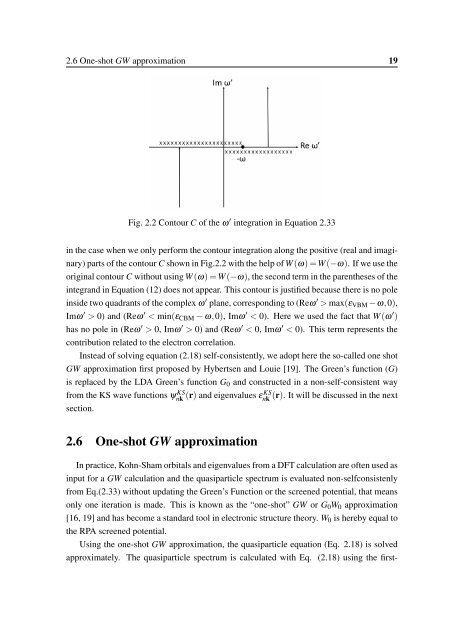
Fig. 2.2 Contour C of the ω ′ integration in Equation 2.33
in the case when we only perform the contour integration along the positive (real and imaginary)
parts of the contour C shown in Fig.2.2 with the help of W(ω) =W(−ω). If we use the
original contour C without using W(ω) = W(−ω), the second term in the parentheses of the
integrand in Equation (12) does not appear. This contour is justified because there is no pole
inside two quadrants of the complex ω ′ plane, corresponding to (Reω ′ > max(ε VBM −ω,0),
Imω ′ > 0) and (Reω ′ < min(ε CBM − ω,0), Imω ′ < 0). Here we used the fact that W(ω ′ )
has no pole in (Reω ′ > 0, Imω ′ > 0) and (Reω ′ < 0, Imω ′ < 0). This term represents the
contribution related to the electron correlation.
Instead of solving equation (2.18) self-consistently, we adopt here the so-called one shot
GW approximation first proposed by Hybertsen and Louie [19]. The Green’s function (G)
is replaced by the LDA Green’s function G 0 and constructed in a non-self-consistent way
from the KS wave functions ψnk KS (r) and eigenvalues εKS
nk
(r). It will be discussed in the next
section.
2.6 One-shot GW approximation
In practice, Kohn-Sham orbitals and eigenvalues from a DFT calculation are often used as
input for a GW calculation and the quasiparticle spectrum is evaluated non-selfconsistenly
from Eq.(2.33) without updating the Green’s Function or the screened potential, that means
only one iteration is made. This is known as the “one-shot” GW or G 0 W 0 approximation
[16, 19] and has become a standard tool in electronic structure theory. W 0 is hereby equal to
the RPA screened potential.
Using the one-shot GW approximation, the quasiparticle equation (Eq. 2.18) is solved
approximately. The quasiparticle spectrum is calculated with Eq. (2.18) using the first-