n?u=RePEc:ais:wpaper:1603&r=his
n?u=RePEc:ais:wpaper:1603&r=his
n?u=RePEc:ais:wpaper:1603&r=his

Create successful ePaper yourself
Turn your PDF publications into a flip-book with our unique Google optimized e-Paper software.
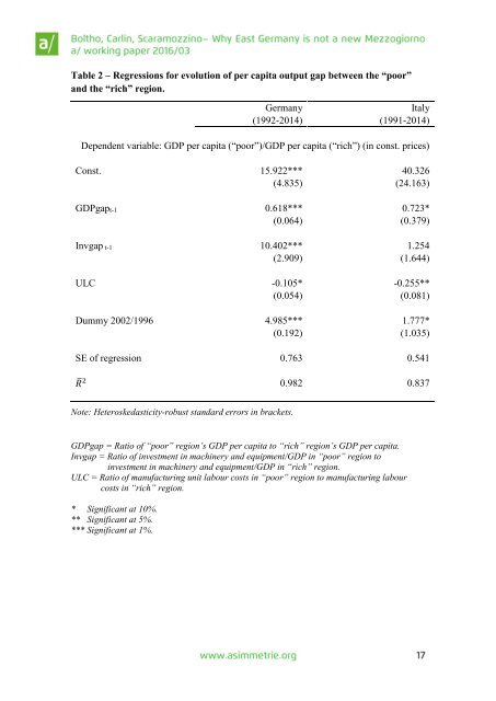
Table 2 – Regressions for evolution of per capita output gap between the “poor”<br />
and the “rich” region.<br />
Germany<br />
Italy<br />
(1992-2014) (1991-2014)<br />
Dependent variable: GDP per capita (“poor”)/GDP per capita (“rich”) (in const. prices)<br />
Const. 15.922*** 40.326<br />
(4.835) (24.163)<br />
GDPgapt-1 0.618*** 0.723*<br />
(0.064) (0.379)<br />
Invgap t-1 10.402*** 1.254<br />
(2.909) (1.644)<br />
ULC -0.105* -0.255**<br />
(0.054) (0.081)<br />
Dummy 2002/1996 4.985*** 1.777*<br />
(0.192) (1.035)<br />
SE of regression 0.763 0.541<br />
R̅2 0.982 0.837<br />
Note: Heteroskedasticity-robust standard errors in brackets.<br />
GDPgap = Ratio of “poor” region’s GDP per capita to “rich” region’s GDP per capita.<br />
Invgap = Ratio of investment in machinery and equipment/GDP in “poor” region to<br />
investment in machinery and equipment/GDP in “rich” region.<br />
ULC = Ratio of manufacturing unit labour costs in “poor” region to manufacturing labour<br />
costs in “rich” region.<br />
* Significant at 10%.<br />
** Significant at 5%.<br />
*** Significant at 1%.