Download Complete Issue - Academic Journals

More documents

Recommendations

Info

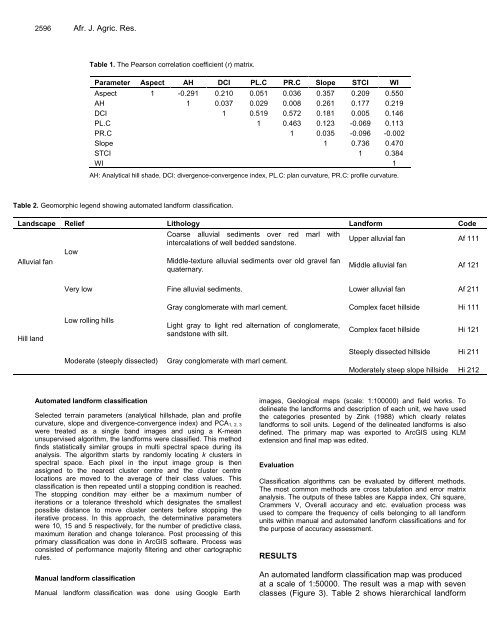
2596 Afr. J. Agric. Res. Table 1. The Pearson correlation coefficient (r) matrix. Parameter Aspect AH DCI PL.C PR.C Slope STCI WI Aspect 1 -0.291 0.210 0.051 0.036 0.357 0.209 0.550 AH 1 0.037 0.029 0.008 0.261 0.177 0.219 DCI 1 0.519 0.572 0.181 0.005 0.146 PL.C 1 0.463 0.123 -0.069 0.113 PR.C 1 0.035 -0.096 -0.002 Slope 1 0.736 0.470 STCI 1 0.384 WI 1 AH: Analytical hill shade, DCI: divergence-convergence index, PL.C: plan curvature, PR.C: profile curvature. Table 2. Geomorphic legend showing automated landform classification. Landscape Relief Lithology Landform Code Alluvial fan Hill land Low Coarse alluvial sediments over red marl with intercalations of well bedded sandstone. Middle-texture alluvial sediments over old gravel fan quaternary. Upper alluvial fan Af 111 Middle alluvial fan Af 121 Very low Fine alluvial sediments. Lower alluvial fan Af 211 Low rolling hills Gray conglomerate with marl cement. Complex facet hillside Hi 111 Light gray to light red alternation of conglomerate, sandstone with silt. Moderate (steeply dissected) Gray conglomerate with marl cement. Automated landform classification Selected terrain parameters (analytical hillshade, plan and profile curvature, slope and divergence-convergence index) and PCA1, 2, 3 were treated as a single band images and using a K-mean unsupervised algorithm, the landforms were classified. This method finds statistically similar groups in multi spectral space during its analysis. The algorithm starts by randomly locating k clusters in spectral space. Each pixel in the input image group is then assigned to the nearest cluster centre and the cluster centre locations are moved to the average of their class values. This classification is then repeated until a stopping condition is reached. The stopping condition may either be a maximum number of iterations or a tolerance threshold which designates the smallest possible distance to move cluster centers before stopping the iterative process. In this approach, the determinative parameters were 10, 15 and 5 respectively, for the number of predictive class, maximum iteration and change tolerance. Post processing of this primary classification was done in ArcGIS software. Process was consisted of performance majority filtering and other cartographic rules. Manual landform classification Manual landform classification was done using Google Earth Complex facet hillside Hi 121 Steeply dissected hillside Hi 211 Moderately steep slope hillside Hi 212 images, Geological maps (scale: 1:100000) and field works. To delineate the landforms and description of each unit, we have used the categories presented by Zink (1988) which clearly relates landforms to soil units. Legend of the delineated landforms is also defined. The primary map was exported to ArcGIS using KLM extension and final map was edited. Evaluation Classification algorithms can be evaluated by different methods. The most common methods are cross tabulation and error matrix analysis. The outputs of these tables are Kappa index, Chi square, Crammers V, Overall accuracy and etc. evaluation process was used to compare the frequency of cells belonging to all landform units within manual and automated landform classifications and for the purpose of accuracy assessment. RESULTS An automated landform classification map was produced at a scale of 1:50000. The result was a map with seven classes (Figure 3). Table 2 shows hierarchical landform
Land classification map Figure 3. Automated landform classification of study area. classification based on Zink method. The results indicated that diverged landforms mostly vary by variation of only two geomorphometric parameters (slope and hill shade). Although, some other parameters have more influence than others in different parts of the study area. For example, Af 121, Af 211 and Af 111 units were mostly separated by slope and partly hill shade factor in alluvial fan landscape. But, all of the used terrain parameters simultaneously affect the separation of landform units in hilly landscape with different intensities. Although, Analytical hill shade parameter has more influence in some landform units located in hilly landscape. In the manual method, eight soil-landscape units (three in the piedmont area and five in the hilly landscape) were identified using the Zink method (Figure 4 and Table 3). Cross tabulation was used for accuracy analysis and evaluation of manual and unsupervised classification (Table 4). Comparison of these methods indicates that: 1) Af 211 unit in manual method is divided into three Moravej et al. 2597 different landform units (Af 111, Af 121 and Af 211) in the automated classification; 2) Hi 211 unit in unsupervised landform classification was not separated in the manual segmentation; 3) Hi 121 and Hi 212 units were delineated with relatively good accuracy in manual and automated methods, respectively; 4) Hi 211 and Hi 212 in the manual method were integrated to Hi 121 and Hi 111 in automated method, respectively; 5) Hi 111 unit in the manual method is divided into two units (Hi 111 and Hi 121) in the automated classification mainly by differences in analytical hill shade parameter; 6) Af 111 unit in automated segmentation was divided to unit (Af 111 and Af 121) in manual segmentation. Although, Af 111 and Af 121 are similar in terrain parameters, but they are different in evolution processes and it is better that they are separated. Important point to consider in comparing the two methods is manual and unsupervised classification can be used complementally for areas that are unavailable or study was limited point of cost and time.
Page 1 and 2: African Journal of Agricultural Res
Page 3 and 4: Editors Prof. N.A. Amusa Editor, Af
Page 5 and 6: Electronic submission of manuscript
Page 7 and 8: Fees and Charges: Authors are requi
Page 9 and 10: Table of Contents: Volume 7 Number
Page 11 and 12: Available online at http://www.acad
Page 13 and 14: diversity and ecosystem productivit
Page 15 and 16: almost with the same species elsewh
Page 17 and 18: Biomass (t/ha) 300 250 200 150 100
Page 19 and 20: plant community. Oikos, 89: 428-439
Page 21 and 22: geomorphologic units such as landsc
Page 23: Figure 2. Hypsometric map of the st
Page 27 and 28: Manual landform classification Figu
Page 31 and 32: The most CTK level was gained in le
Page 33 and 34: Table 4. Comparison of average effe
Page 35 and 36: existed in amino acids and other pr
Page 39 and 40: Table 3. Characteristics of the use
Page 41 and 42: V0 0 V1 10 Vermicompost concentrati
Page 43 and 44: Stem height (cm) V0 0 V1 10 V2 20 V
Page 45 and 46: Leaf (number) V0 0 V1 10 V2 20 V3 3
Page 47 and 48: Flowering (days) V0 0 V0 0 V1 10 V2
Page 49 and 50: Edwards CA, Arancon NQ, Vasko-Benne
Page 51 and 52: about 366 ppm in 1998 (FAO, 2001).
Page 53 and 54: Statistical analysis The statistica
Page 55 and 56: Table 2. Soil EC, pH, calcite, SOC,
Page 57 and 58: area is 7.4 indicating the moderate
Page 59 and 60: Vacca A, Loddo S, Erra G, Aru A (20
Page 61 and 62: (GPMP) also exhibit significant bio
Page 63 and 64: Liver index (%) 4.5 4 3.5 3 2.5 2 1
Page 65 and 66: (MDA) has been the most widely used
Page 69 and 70: to analyse similar studies on lives
Page 71 and 72: Table 2. Parameter estimates of the
Page 73 and 74: ased on a cross-sectional household
Page 75 and 76:
African Journal of Agricultural Res
Page 77 and 78:
parasites (1.2%; n = 1), predation
Page 79 and 80:
et al., 2004), Ethiopia (Halima, 20
Page 81 and 82:
Page 83 and 84:
Table 1. The evaluation system of i
Page 85 and 86:
AI(CNY) AI (CNY) area (ha) Area (ha
Page 87 and 88:
YRPA/YFGPA(kg/hm 2 ) YRPA/YFGPA (kg
Page 89 and 90:
NBI/PBIK/REOI NBI/PBIK/REOI 6.0 5.0
Page 91 and 92:
only improved but also increased. T
Page 93 and 94:
discounted this direct relationship
Page 95 and 96:
Plant available water (%) Wakindiki
Page 97 and 98:
Page 99 and 100:
Figure 1. Bulblet regeneration from
Page 101 and 102:
obtained with a medium containing 2
Page 103 and 104:
Table 1. Descriptive statistics of
Page 105 and 106:
Table 5. Standardized coefficients
Page 107 and 108:
Page 109 and 110:
Figure 2. F-actin and the movement
Page 111 and 112:
Page 113 and 114:
Figure 2. Reciprocating mechanism.
Page 115 and 116:
Table 1. Program for controlling th
Page 117 and 118:
Page 119 and 120:
TC it �� f ( xis, s, �)
Page 121 and 122:
Table 3. Parameter estimates of the
Page 123 and 124:
alone. The efficiency scores are pa
Page 125 and 126:
Indices TFP index 1.20 1.10 1.00 0.
Page 127 and 128:
Table 7. TFP grow th and its compon
Page 129 and 130:
Page 131 and 132:
secondary literature and key inform
Page 133 and 134:
Table 3. Farmers’ knowledge and a
Page 135 and 136:
Table 7. Varieties grown by farmers
Page 137 and 138:
Table 11. Reasons why farmers do no
Page 139 and 140:
ACKNOWLEGEMENTS The authors are gra
Page 141 and 142:
Page 143 and 144:
Precipitation (mm) 55 50 45 40 35 3
Page 145 and 146:
The increase in pH in the treatment
Page 147 and 148:
organic manure and fertilizers on c
Page 149 and 150:
Conferences and Advert September 20
show all

Download Complete Issue - Academic Journals

You also want an ePaper? Increase the reach of your titles

Delete template?

Save as template?