The OTIS Reference Manual - Hasylab

7.2 OTIS1.1 Sample Measurements
Digital to Analog Converter:
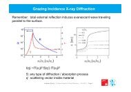
Figure 10 shows the behavior of the 4 digital to analog converters which provide the threshold
voltages for the ASD discriminator chips. The outputs of the DACs are now buffered and therefore
able to drive currents up to 600µA. Figure 10 shows how the output voltages at an external
load (1.2kOhm) vary with programming of the DAC registers. Extra design effort went into chip
version OTIS1.2 in order to decrease the spread in between all 4 channels (which is ≈80mV for
OTIS1.1).
Output Voltage [mV]
2500
2000
1500
1000
500
Digital to Analog Converter
1.2kOhm load
DAC 0
DAC 1
DAC 2
DAC 3
0
0 50 100 150 200 250
Bin Number
Figure 10: DAC Measurement
Vctrl [mV]
2500
2000
1500
1000
500
DLL Lock Range
(Room Temperature)
0
20 30 40 50 60
Clock Frequency [MHz]
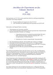
Figure 11: DLL Lock Range
DLL Lock Range:
Figure 11 combines data from 2 different measurements concerning the lock range of the DLL. The
diagram shows the control voltage of the single delay elements against the LHC clock frequency.
Data from 25MHz to 46MHz has been obtained with standard chip settings. The chip operated
at a different supply voltage (Vdda = 3.3V instead of 2.5V) from 47MHz to 60Mhz. The resulting
offset in Vctrl has been taken into account for this summary. At room temperature and provided
that reset is active before the clock is running, the DLL reaches its lock state for clock frequencies
that range from 25MHz to 60MHz.
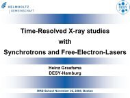
Drift Time Measurement:
Figure 12 shows the linear dependency between input signal delay (x-axis) and drift times (y-axis)
derived from the input signal. The drift time data that contribe to this figure ranges from 0 to
63. Thus data only represents an overall drift time range of 25ns. In this diagram 0ns drift times
belong to an input signal delay of 6ns and range to 24.9ns (resp. 30.9ns input signal delay). The
drift time figures repeat below an input signal delay of 6ns and above a delay of 30.9ns .
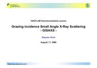
Differential Non-Linearity:
To calculate a figure for the differential non-linearity, several million drift times derived from random
input signals need to be stored and analyzed. The DLL bin sizes can be calculated from the
histogram of all drift times. Now the difference in bin size of always two subsequent DLL bins
can be calculated. But one needs to take into account that always two bins of different size form
one delay element of the DLL. A sample diagram displaying bin size differences against the bin
number is shown in figure 13. Now the sum of the biggest and (the absolute value of the) smallest
bin size difference is called differential non-linearity. The data of diagram 13 results in a DNL of
(1.25 ± 0.04)LSB or (489 ± 16)ps. The dominating contribution to the DNL originates from an
18