Energy consumption modelling - ADU-RES

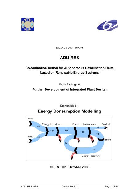
INCO-CT-2004-509093 

ADU-RES 

Co-ordination Action for Autonomous Desalination Units 

based on Renewable Energy Systems 

Solar 

Wind 

Work Package 6 

Further Development of Integrated Plant Design 

Deliverable 6.1 

Energy Consumption Modelling 

60 

40 

Energy In Motor Pump Membranes Product 

100 80 

115 

20 

70 

20 

15 25 

Brine 

50 

MSankeyW 

20 

CREST UK, October 2006 

70 

Energy Recovery 

ADU–RES WP6 Deliverable 6.1 Page 1 of 69

Work Package 6 Participants 

Organization Participant Researchers 

Murray Thomson 

CREST, Loughborough University, U.K. Alfredo Bermudez 

David Infield 

Fraunhofer ISE, Germany Joachim Went 

Agricultural University of Athens (AUA), 

Greece 

Costas Soulis 

Centre for Renewable Energy Sources, 

(CRES), Greece 

Eftihia Tzen 

Joint Research Centre (JRC), EU 

Neringa Narbutiene 

Robert Edwards 

Instituto Tecnológico de Canarias, 

(ITC), Spain 

Baltasar Peñate Suarez 

Vicente Subiela Ortin 

Gonzalo Piernavieja Izquierdo 

Project Coordination 

Dr Christian Epp 

Michael Papapetrou 

WIP – Renewable Energies 

Sylvensteinstrasse 2, 81369 Munich, Germany 

christian.epp@wip-munich.de 

michael.papapetrou@wip-munich.de 

Tel: 0049 89 720 12 735 

This report prepared by 

Murray Thomson 

Alfredo Bermudez 

CREST (Centre for Renewable Energy Systems Technology) 

Loughborough University 

Loughborough, LE11 3TU, United Kingdom 

M.Thomson@Lboro.ac.uk 

Tel: 0044 1509 228144 

with specific technical assistance from 

Eftihia Tzen 

Centre for Renewable Energy Sources, (CRES) 

Greece 

and 

Vicente Subiela Ortin 

Baltasar Peñate Suarez 

Instituto Tecnológico de Canarias (ITC) 

Pozo Izquierdo, Gran Canaria Island 


Contents 

1 Introduction...............................................................................................4 

2 Energy in RO systems ..............................................................................5 

2.1 Concentration ....................................................................................5 

2.2 Osmotic pressure ..............................................................................5 

2.3 Theoretical minimum desalination energy .........................................5 

2.4 Pre-treatment losses .........................................................................6 

2.5 Membrane losses ..............................................................................7 

2.6 Concentrate energy ...........................................................................8 

2.7 Specific energy (kWh/m 3 ) ................................................................10 

3 Modelling methodology...........................................................................11 

3.1 Software ..........................................................................................11 

3.2 Input data.........................................................................................12 

3.3 Photovoltaics (PV) ...........................................................................12 

3.4 Maximum power point tracking (MPPT)...........................................12 

3.5 Charge controllers ...........................................................................13 

3.6 Wind turbines...................................................................................13 

3.7 Batteries ..........................................................................................13 

3.8 Power electronic converters (including inverters) ............................13 

3.9 Induction motors ..............................................................................14 

3.10 Centrifugal pumps ...........................................................................14 

3.11 Positive displacement pumps ..........................................................14 

3.12 DC motor-pumps .............................................................................14 

3.13 Membranes......................................................................................14 

3.14 Clark pump ......................................................................................14 

3.15 Filter and pipe losses.......................................................................15 

3.16 Flushing, cleaning, fouling and scaling ............................................15 

4 ITC DESSOL Seawater PV-RO, Gran Canaria.......................................16 

4.1 Assumed details ..............................................................................17 

4.2 The completed model ......................................................................21 

4.3 Modelled performance – without the well pump...............................23 

4.4 Modelled performance – including the well pump............................28 

5 CRES Seawater PV-Wind-RO, Lavrio, Greece.......................................31 


5.2 Modelled performance.....................................................................38 

6 CREST Seawater PV-RO .......................................................................42 

6.1 System details .................................................................................43 


7 CREST Seawater Wind-RO, UK.............................................................50 

7.1 System details .................................................................................51 


8 ITN Brackish PV-RO, Mesquite, Nevada ................................................54 



9 INETI Brackish PV-RO, Portugal ............................................................61 



10 Conclusions and recommendations ....................................................68 


1 Introduction 

Many demonstration ADU-RES systems have been constructed and operated 

in recent years. In all cases, the quantity of water produced is modest in 

relation to the size of the solar collectors, wind-turbines or other renewableenergy 

collection equipment. Ultimately, this makes the water expensive and 

is the main factor constraining the commercial uptake of ADU-RES. 

The problem is largely due to energy losses in each of the individual 

components that make up ADU-RES systems. In fairness, similar losses are 

also prevalent in small-scale fossil-fuelled desalination systems, but often go 

unnoticed because the capital costs of internal combustion engines (or 

alternatives) are relatively low. 

This report presents modelling of energy flows in a selection of ADU-RES 

systems. The aim is to quantify the energy losses in the various components 

and thus indicate where attention should be focused in order to reduce those 

losses in future system designs. 

The selected systems include solar photovoltaics (PV) and wind power; they 

are all based on reverse osmosis (RO). 


2 Energy in RO systems 

This section describes the fundamentals of energy consumption in RO 

systems. 

2.1 Concentration 

The concentration of salts in the feed water is the primary factor determining 

the energy required for desalination. 

Average seawater has a total-dissolved-solids concentration of 35 750 mg/L. 

Some seas have significantly higher concentrations, notably the Red Sea and 

Arabian Gulf, which can be up to 45 000 mg/L, and therefore require more 

energy to desalinate. 

Brackish groundwaters (concentrations typically less than 10 000 mg/L) 

generally require much less energy. 

2.2 Osmotic pressure 

Osmotic pressure is roughly proportional to concentration. 

The exact relationship is a complex function of the concentrations of each of 

the ions present in the water, but for a basic appreciation of energy flows, it is 

sufficient to know that doubling the concentration will roughly double the 

osmotic pressure, and a similar doubling of energy consumption can be 

expected. 

2.3 Theoretical minimum desalination energy 

The theoretical minimum energy required to remove salt from water is 

independent of the method employed and is directly related to the osmotic 

pressure: 

1 bar = 1/36 kWh/m 3 

Average seawater has an osmotic pressure of around 26 bar, which equates 

to just over 0.7 kWh/m 3 . 

In practice however, the osmotic pressure increases as the desalination takes 

place: the removal of fresh water causes the feed water to become 

concentrated. Thus, the energy required to remove the salt increases, 

depending on the recovery ratio, as indicated in Figure 1. 


Minimum Energy (kWh/m 3 ) 

3.5 

3 

2.5 

2 

1.5 

1 

0.5 

0 

0 10 20 30 40 50 60 70 80 90 100 

Water Recovery Ratio (%) 

Figure 1 – Theoretical minimum energy required to desalinate 

seawater at 25 ºC 1 

The above discussion, including Figure 1, refers to the complete removal of 

salt, which is not generally necessary in the production of drinking water. 

Product concentrations of up to 600 mg/L can be acceptable and this slightly 

reduces the energy required. The reduction is usually insignificant in seawater 

systems but is worth noting in the case of brackish water. 

The temperature of the water also has a slight affect: osmotic pressure is 

roughly proportional to absolute temperature in Kelvin. This factor is generally 

insignificant in RO systems and should not be confused with the temperature 

dependence of RO membranes. 

2.4 Pre-treatment losses 

Almost all practical RO systems include some form of pre-treatment. Usually, 

this includes filtration, and requires energy to overcome the associated 

pressure drops. Provided that filters are appropriately sized and properly 

maintained, the energy required is generally small compared to that for the 

actual desalination and is not included in the modelling presented here. 

1 Johnson, James S., Lawrence Dresner and Kurt A. Kraus (1966). Hyperfiltration (Reverse 

Osmosis). Principles of Desalination. K. S. Spiegler. New York, Academic Press, page 357. 


2.5 Membrane losses 

Energy losses in RO membranes can be divided into through-flow losses and 

cross-flow losses. 

Through-flow losses 

An ideal RO membrane would form a complete barrier to salt ions but would 

allow water to pass through freely. In this case, the energy consumption 

would be solely due to the osmotic pressure, as discussed above. With a real 

membrane however, the feed pressure has to be greater than the osmotic 

pressure in order to push the water through the membrane. This additional 

pressure is known as the “net driving pressure” and corresponds to additional 

energy, which is dissipated as heat and lost. 

This energy loss is proportional to the net driving pressure and can thus be 

reduced by reducing the system feed pressure. To minimise the energy loss, 

the system feed pressure should be only slightly above the osmotic pressure 

of the concentrate, and it is notable that the (traditionally powered) RO 

systems with the lowest energy consumptions do operate at relatively low 

pressures. 

On the other hand, the flow (quantity) of product water is also roughly 

proportional to the net driving pressure, and thus, the system designer must 

balance the conflicting objectives of minimising the energy losses described 

above against maximising the product flow. 

The situation can be improved by use of a large membrane area (extra 

membrane modules), and again, it is notable that RO systems designed to 

minimise energy consumption do tend to have a generous number of 

modules. The benefit of reduced energy costs has to be set against the 

increased capital and replacement costs of membranes, and an increase in 

product concentration. 

Membrane manufactures also seek to minimise the energy loss described 

above, by designing membranes to allow water to pass through as freely as 

possible. Membranes designed with this priority are described as “high-flow” 

or “low-pressure” membranes. Unfortunately, but unsurprisingly, these 

membranes also tend to allow slightly more salt to pass through. Membranes 

designed to minimise salt passage are described as “high-rejection”, and are 

less energy efficient. 


Cross-flow losses 

Cross-flow losses correspond to the pressure drop between the feed inlet to 

the membranes and the concentrate outlet, sometimes known as the “delta 

pressure”. 

In energy terms, cross-flow losses are usually small in comparison to throughflow 

losses. 

Through-flow and cross-flow losses are calculated separately in the modelling 

described in this report, but they are combined in the presented results. 

2.6 Concentrate energy 

The concentrate exiting the membranes of an RO system has hydraulic 

energy by virtue of its flow and pressure. 

In seawater systems, this energy is very significant: typically equal to around 

two thirds of the energy presented to the membranes at the feed intake. 

High-pressure 

seawater 

feed 

Reverse-Osmosis Modules 

3 

3 

3 m /h 

1m/h 

at 60 bar 

Concentrate 

Brine 

Reject 

3 

2m/h 

at 59 bar 

Freshwater 

Product 

Permeate 

Figure 2 – Example to illustrate concentrate energy in seawater RO 

Large and medium-scale (traditionally powered) seawater RO systems are 

almost always equipped with “brine-stream energy recovery”. The traditional 

mechanism was a Pelton wheel coupled to the shaft of the main feed pump. 


Electricity 

Seawater 

Motor 

Pump 

Pelton 

wheel 

60 bar 

RO Modules 

Concentrate Brine 

59 bar 

Freshwater 

Product 

Permeate 

Figure 3 – Use of a Pelton wheel in a large (traditionally powered) RO system 

In recent years, alternative brine-stream energy recovery mechanisms have 

been developed and widely employed in large and medium-scale RO 

systems. These include the DWEER Work Exchanger 2 and the ERI Pressure 

Exchanger 3 . 

Unfortunately, the devices mentioned above are not readily available at smallscale 

(product flow below ~ 50 m 3 /d) and the vast majority of small-scale RO 

systems are fitted with a needle valve to provide the necessary backpressure 

to the membranes. The concentrate energy is dissipated as heat in the needle 

valve and lost. As a result, the relative energy consumption in these systems 

is very high. 

Various devices have been developed for and applied to brine-stream energy 

recovery in small-scale RO systems. These include the Clark pump 4 , which 

has been very successful in use on leisure yachts, and the Danfoss axialpiston 

motor (APM) 5 . Unfortunately, these devices cost rather more than a 

simple needle valve and their potential to save on-going energy costs is often 

overlooked. 

Brackish water RO systems usually operate at a higher (water) recovery ratio 

than seawater systems. Thus, the proportion of the energy in the concentrate 

is lower and the importance of brine-stream energy recovery is reduced. 

2 www.calder.ch 

3 www.energy-recovery.com 

4 www.spectrawatermakers.com 

5 http://nessie.danfoss.com 


2.7 Specific energy (kWh/m 3 ) 

Dividing the energy consumption of an RO plant in kW by the product flow in 

m 3 /h yields the “specific energy” in kWh/m 3 , and provides a convenient basis 

for comparing energy consumption in plants of different capacities. Some 

typical figures are given in Table 1. 

Specific energy 

(kWh/m 3 ) 

Without energy recovery 5 – 10 

With energy recovery 2 – 4 

Theoretical minimum ~ 1 

Table 1 – Typical energy consumptions for medium and large-scale 

traditionally powered seawater RO 

It should be emphasised however that specific energy figures depend greatly 

on where the energy is being measured and what it includes. In a gridpowered 

RO system, the designer may focus on the energy consumption of 

the motor driving main high-pressure-pump and perhaps overlook auxiliary 

loads such as a well pump. With an autonomous system on the other hand, 

there is a greater obligation to include all aspects of energy consumption, and 

thus, specific energy figures will appear higher. 

System size also has a significant bearing on specific energy consumption. 

The energy efficiencies of small electric motors and pumps are very much 

less than larger machines. Also, parasitic losses, such as measurement and 

control equipment, will be a more significant proportion of the total energy 

consumption. Fortunately, the energy efficiency of the membranes 

themselves is almost unaffected by system size: the membrane material used 

in a single 2.5-inch or 4-inch element in a very small RO system is identical to 

that used in the multiple 8-inch to 18-inch elements of a municipal RO system. 

The care and cleaning of the membranes however, which is required equally 

in all systems, might not be carried out so carefully carried out in small 

systems, and this will lead to a more rapid decline in performance, including a 

rise in specific energy. 


3 Modelling methodology 

The software models presented in this report are intended to simulate the 

energy flows and water production of the real demonstration systems on 

which they are based. The models are based on information taken from 

numerous published and unpublished sources. In many cases, additional 

information was required in order to complete the model and assumptions 

were made. The assumed details are described for each of the modelled 

systems. This section describes the general approach to the modelling of all 

systems. 

3.1 Software 

The models are written in Matlab-Simulink, which is a general-purpose 

simulation tool used worldwide in engineering and academic research. It can 

be used to develop very detailed time-step simulations of complex physical 

systems, and is vastly more powerful than Excel. Of course the quality of the 

results is still critically dependent on the quality of the model construction and 

the data used as input. 

The general arrangement of the Matlab-Simulink models follows the approach 

taken previously by Thomson 6 and Miranda 7 , which proved very successful in 

predicting specific energy consumption of the ADU-RES system at CREST. 

This approach to the modelling allows the behaviour of each component to be 

represented in detail. For example, the model of a centrifugal pump can 

include accurate pressure-flow and energy-efficiency curves representing the 

full range of its operation. A simple model constructed in Excel would tend to 

use single-point parameters, which may not be accurate when the pump is 

operated under differing conditions. 

Matlab-Simulink facilitates time-series simulation, and the models presented 

in this report are configured to simulate hour-by-hour operation for a complete 

year. This level of detail is important in order to accurately represent the 

operation of ADU-RES systems with variable energy inputs. In systems with 

batteries, the state-of-charge and cell voltages are calculated at each time 

step and used to determine the on/off operation of the RO section. In systems 

without batteries, flows and pressures throughout the RO section vary in 

6 Thomson, Murray (2004). Reverse-Osmosis Desalination of Seawater Powered by 

Photovoltaics Without Batteries, PhD, University of Loughborough, UK. 

http://www-staff.lboro.ac.uk/~elmt/Thesis.htm 

7 Miranda, Marcos S. (2003). Small-Scale Wind-Powered Seawater Desalination Without 

Batteries, PhD, Loughborough University, UK. http://staff.bath.ac.uk/eesmm/Thesis.html 


esponse to the variable energy input and this is fully represented in the 

modelling. 

Selection of a 1-hour time-step facilitates simulation of a whole year of 

operation so that seasonal and weather variations can be represented. 

Variations occurring within an hour, such as passing clouds affecting the solar 

input and wind turbulence, are not represented, but trial simulation runs using 

shorter time-steps have shown no significant differences in overall results. 

3.2 Input data 

The real demonstration systems (on which the models are based) are located 

in various countries, and naturally, their performance is very dependent on 

local conditions: 

• Solar radiation 

• Wind speed 

• Feed water concentration and temperature 

• Ambient temperature 

The software models use hourly data to represent these variables, and the 

details of the data sources are given in the “assumed data” section for each 

system. 

3.3 Photovoltaics (PV) 

Ambient temperature and solar radiation data is used to model cell 

temperature using NOCT 8 . The operation of each PV cell is then represented 

by a one or two-diode model, calibrated to match the manufacturer’s 

published current-voltage (I-V) curves for the module. 

The series-parallel configuration of the array is represented by simple 

multiplication of currents and voltages. No allowance is made for mismatch 

and shading losses; these losses should be small provided that good-quality 

modules are installed in open aspect and kept clean. 

3.4 Maximum power point tracking (MPPT) 

The maximum power point is determined from the I-V curve mentioned above. 

The model assumes that the tracking algorithm is perfect: no tracking errors. 

Losses in the DC-DC or DC-AC power-electronic converter are modelled 

appropriately. 

8 

Normal Operating Cell Temperature (NOCT), see Markvart, Tomas (1999), Solar Electricity. 

Chichester, Wiley, page 88. 


3.5 Charge controllers 

Charge controllers do not perform maximum power point tracking; they simply 

disconnect the PV from the battery when the state-of-charge (indicated by the 

battery voltage) exceeds a threshold and thus prevent overcharging. Some 

charge controllers use pulse-width modulation (PWM) to provide float and 

equalisation charging, but as the model operates on a 1-hour time-step, these 

details of are not of importance here. 

In a PV-RO system, a charge controller serves only as a backup to prevent 

overcharging: in normal operation, the RO rig will be switched on at a 

threshold below that of the charge controller. Thus, it was not necessary to 

specifically include charge controllers in the models. 

In the absence of maximum power point tracking, the battery voltage is simply 

applied to the PV, and the current at that voltage is calculated from the I-V 

curve mentioned above. In general, the battery voltage will differ from the 

MPP voltage and thus the PV will deliver less energy than it could. This 

energy loss is indicated “No MPPT” in the Sankey diagrams shown later. 

3.6 Wind turbines 

The wind turbines models are based on power curves (electrical output power 

versus wind speed). It should be noted, however, that measurement of power 

curves for small wind turbines is notoriously difficult and field performance 

often falls short of manufacturer’s curves. 

The curves also assume that the turbine rotational speed is well controlled to 

match the wind speed, which is not always the case. 

3.7 Batteries 

Charging and discharging losses are modelled according to manufacturer’s 

data at specified charge/discharge rates (C50, C100 etc.). This provides a 

state-of-charge estimate, which is used to determine cell voltage, again 

allowing for charge/discharge rate. Ambient temperature and battery ageing 

are not included in the model; these could be significant in the life of an ADU- 

RES system. 

3.8 Power electronic converters (including inverters) 

Losses in DC-DC converters and DC-AC inverters are a function of power 

flow (or current) and these are modelled based on manufacturer’s efficiency 

curves wherever possible. Additional losses in motors, generators and 

batteries due to harmonics caused by power electronic converters are not 

modelled but should be small provided that good-quality converters are used. 


3.9 Induction motors 

Efficiency curves for induction motors are based on actual manufacturer’s 

data, supplemented by data for very similar motors manufactured by Brook 

Crompton 9 . Power factors of three-phase motors are similarly modelled as a 

function of operating power. Power factors of single-phase motors are harder 

to predict, because capacitor and winding arrangements differ between 

manufacturers. They were treated as constants between 0.96 and 0.98. Any 

errors have only a second-order effect on energy losses: reactive current will 

cause small losses in power electronic converters. 

3.10 Centrifugal pumps 

The efficiency of centrifugal pumps is critically dependent on operating point. 

This is modelled through application of the manufacturer’s head-flow and 

power-flow curves. In some cases, data from very similar Grundfos pumps 

was substituted. 

3.11 Positive displacement pumps 

The geometric displacement, taken from the manufacturer’s data, is used to 

calculate ideal flow and torque. Volumetric and mechanical efficiency curves 

are then applied to determine losses as a function of operation point. 

3.12 DC motor-pumps 

The DC motors in the selected systems are integrated with their respective 

pumps and were modelled using manufacturer’s performance curves for the 

complete units. 

3.13 Membranes 

The models of the RO elements in the Matlab/Simulink model are derived 

from Dow FilmTec's ROSA 10 . 

3.14 Clark pump 

The Clark pump model is based on detailed in-house measurements made 

over a broad range operation 11 . 

9 www.brookcrompton.com 

10 http://www.dow.com/liquidseps/design/rosa.htm 

11 Thomson, Murray (2004). Reverse-Osmosis Desalination of Seawater Powered by 

Photovoltaics Without Batteries, PhD, University of Loughborough, UK. 

http://www-staff.lboro.ac.uk/~elmt/Thesis.htm Section 5.2 


3.15 Filter and pipe losses 

Pressure losses in filters and pipes are not included in the model. They are 

expected to be small, provided that filters are kept clean, pipe diameters are 

adequate, lengths are kept short and sharp elbows are avoided. 

3.16 Flushing, cleaning, fouling and scaling 

Flushing and cleaning directly affect the overall specific energy consumption 

in two ways: 

• Energy is consumed by the pumps used during flushing and cleaning. 

• Product water is consumed, reducing the overall system output. 

All RO systems require flushing and cleaning (or have to accept very frequent 

membrane replacement), but quantifying this and the resulting decline in 

membrane performance is beyond the scope of the modelling presented here. 

RO systems operating intermittently, with variable flow or at relatively low 

flows may be more prone to fouling than those operating at continuous high 

flow. 


4 ITC DESSOL Seawater PV-RO, Gran Canaria 

Photovoltaic 

array 

Charge 

regulator 

DC 

Batteries 

Inverter 

AC 

Induction 

motor 

Seawater 

Well 

Induction 

motor 

Plunger 

pump 

Centrifugal 

pump 

RO membranes 

Optional 

Figure 4 – General Arrangement – ITC DESSOL Seawater PV-RO, Gran Canaria 

Needle 

valve 

Fresh water 

product 

Concentrate 

discharge 


4.1 Assumed details 

The details given here were used for the modelling described in this report and may differ from those of the actual installed system. 

The model is based on the system operated by ITC, Pozo Izquierdo, Gran Canaria 12 . 

The actual system does not have the well pump shown in Figure 4; instead, it is fed by a general site supply of seawater, which is 

pumped using grid electricity. The centrifugal well pump shown in Figure 4 is the proposed supply method for an autonomous 

system. The modelling was completed both with and without this well pump. 

RO operational parameters 

Product flow 400 L/h 

Recovery Ratio 45 % 

Feed flow 900 L/h 

Working pressure 55 bar 

Seawater feed 

Concentration 35 500 ppm TDS 

…Osmotic pressure 26.3 bar 

Temperature 19 °C to 23 °C 

Solar radiation 

Annual average: 

On a horizontal surface 5.6 kWh/m 2 /d 

Inclined at 10 degrees 5.8 kWh/m 2 /d www.cabildodelanzarote.com/energias/gonzalopiernavieja.pdf - page 40 

Hourly data Meteonorm http://www.meteotest.ch/ 

And scaled to give an annual average of 5.8 kWh/m 2 /d. 

Ambient temperature (for PV) 


12 ADU-RES, Work Package 2, Final Report, section 4.3.2. 


Photovoltaic array 

Nominal array power 4.8 kWpeak 

Number of modules 64 

Wiring configuration 16 strings each comprising 4 modules in series 

Nominal module power 75 Wpeak 

Module type Mono-crystalline 

Manufacturer Atersa www.atersa.com 

Model A-75 www.heliplast.cl/pdf/a75m.pdf 

Cells per module 36 in series 

MPP voltage 17.0 V 

Batteries 

Type Flooded lead-acid 

Manufacturer Fulmen Solar 

Capacity 400 Ah at 100 h rate 

Configuration 24 cells in series 

Nominal overall voltage 48 V 

Nominal energy capacity 19.2 kWh 

Assume performance details from: 

Manufacturer BP Solar www.bpsolar.com.au 

Model PVSTOR 2P430 http://www.bp.com/... /Aust_ps_solar_PVstorBrochure.pdf 

Capacity 430 Ah at 100 h rate www.solartech.com.au/pdfs/products/batteries/pv_stor_manual_5.pdf 

Inverter 

Manufacturer Trace, Xantrex www.xantrex.com 

Model SW4548E SW Series Inverter/Chargers – (4.01 Software Revision) User Guide 

Nominal Input 48 V, DC http://www.xantrex.com/web/id/610/docserve.asp 

Output 230 V, 50 Hz, Single-phase 

Rated power 4500 VA 

Efficiency (peak) 96 % 

Efficiency curve From User Guide Figure 19 


Motor (for plunger pump) 

Type 4-pole Single-phase induction 

Power 2.2 kW 

Assume other parameters similar to: 

Manufacturer Brook Crompton 

Model TDA100LZ (4-pole, low running current) www.brookcrompton.com/pdf-files/2227e_1phase_v1.1e.pdf 

Rated speed 1430 rpm 

Rated current 13.0 A 

Efficiencies 78 % at full load, 76 % at ¾ load, 71 % at half load 

Power factor 0.96 (assumed constant) 

Belt drive (for plunger pump) 

Ratio 0.62 To give rated pump speed at rated motor speed. 

Efficiency 97 % (assumed) 

Plunger pump 

Manufacturer CAT www.catpumps.com 

Model 317 http://www.catpumps.com/select/pdfs/317.pdf 

Rated flow 15 L/m = 900 L/h 


Volumetric and mechanical efficiency curves from CREST’s own testing of a CAT 317. 

RO membranes 

Type Spiral-wound, polyamide thin-film composite, for seawater 

Element size 2.5 inch by 40 inch 

Number of elements 12 

Configuration 2 parallel trains of 6 series elements 

Manufacturer Dow FilmTec http://www.dow.com/liquidseps/ 

Model SW30-2540 http://www.dow.com/liquidseps/prod/sw30_2540.htm 

Performance details ROSA http://www.dow.com/liquidseps/design/rosa.htm 


Well pump (centrifugal) 

As noted above, the well pump is the proposed supply method for an autonomous system. The demonstration system at ITC does 

not have its own well pump. 

Rated pressure 3 bar 

Rated flow 2.5 m³/h 

Rated power 1 kW 

Depth (head) 4 m 

Manufacturer Grundfos www.grundfos.com 

Model CRT 2-5 Data booklet No.:V7149894, Grundfosliterature-942.pdf 

Motor (for well pump) 

Manufacturer Grundfos 

Type 2-pole induction motor 

Rated (output) power 0.55 kW 

Full load efficiency 65 % 

Efficiency curve and other details based on: 

Manufacturer Brook Crompton www.brookcrompton.com/pdf-files/2227e_1phase_v1.1e.pdf 

Model 2-TDA71MR (2-pole) 


4.2 The completed model 

Irradiance 

Temperature 

Hourly Data 

PozoIzquierdo 

G 

Ta 

V 

PV Array 

I 

SoC 

Ia 

V 

V 

Io 

Charge 

Regulator 

Ipv 

Iro 

SoC 

Batteries 

35500 

G 

SoC 

Feed Concentration 

Run 1/0 

Rig Control 

Tf 

Feed Temperature 

Vdc 

Cf 

Tf 

Inverter 

& RO Rig 

Figure 5 – Top level of Matlab-Simulink model of ITC DESSOL Seawater PV-RO 

The data outlined in the previous section was used to construct a Matlab-Simulink model of the complete system using the 

approach outlined in Section 3. The model simulates one complete year of operation on an hour-by-hour basis. The model includes 

a controller that runs the RO rig according to the available solar radiation and the battery state of charge. Thus, the daily water 

ADU–RES WP6 Deliverable 6.1 Page 21 of 69 

V 

Idc 

Qp 

Cp 

Q 

C 

Product 

Tank

production varies according to the solar radiation data. The annual water production is logged and used to calculate annual 

average specific energies throughout the system. 

Enable 

1 

Vdc 

Inverter 

Vdc 

Iac 

pf 

Idc 

Vac 

f 

1 

Idc 

AC Bus 

I1 

pf 1 

V 

f 

I2 

pf 2 

V 

f 

I 

pf 

V 

f 

Motor P 

T 

V 

f 

T 

V 

f 

n 

I 

pf 

Motor C 

n 

I 

pf 

n 

Q 

nM 

TP 

Centrifugal Pump 

T 

P 

Belt 

TM 

nP 

Well Pipe 

Q 

Pb 

Pt 

Q 

Plunger Pump 

n 

T 

Qf, m3/h 

Pc, bar 

Cf 

RO Membranes 

Tf , degC 

Figure 6 – Contents of the “Inverter and RO Rig” block shown in Figure 5 

Po 

Pi 

Q 

2 

Cf 

3 

Tf 

Pf , bar 

Qc, mg/L 

Cp, mg/L 

Qp, m3/h 

3 

Cp 

2 

Qp 

4.4 

Needle Valve 

The individual component blocks shown in Figure 6 correspond to the hardware components shown earlier in Figure 4. The 

arrowed lines connecting the component blocks in Figure 6 represent the flows, pressures, voltages, currents, etc. in the respective 

pipes and wires of the real system. The arrows indicate the direction of the data flow, not the actual directions of water or current 

flow. 

Notice that in many cases the arrowed lines carry the data backwards and thus form “algebraic loops”. This is a natural 

consequence of a physically interconnected system. Matlab-Simulink uses an iterative solver to perform such calculations. 

ADU–RES WP6 Deliverable 6.1 Page 22 of 69 

App, % 

Q 

P

The contents of the individual component blocks perform the detailed calculations according to the efficiency curves etc. outlined in 

the preceding section. 

4.3 Modelled performance – without the well pump 

General results from the model 

Annual energy available from PV 8820 kWh/y 

Annual hours run 2935 h/y 

Average hours run per day 8.09 h/d 

Annual water production 1200 m 3 /y 

Average daily water production 3.29 m 3 /d 

Overall annual average specific energy 8820/1200 = 7.35 kWh/m 3 

The above figures, particularly the average hours run per day and the average daily water production show good agreement with 

the figures reported by ITC for the real demonstration system. 

The overall specific energy figure shown above is calculated from the energy available from the PV. It is therefore higher that the 

figure of 5.5 kWh/m 3 measured by ITC at the input to the plunger pump motor (see also the following discussion). 


Sankey diagram 

7.35 

PV Inverter 

0.73 

2.07 

4.55 

No MPPT 

Battery 

1.16 

0.9 

0.39 

5.06 

Feed 

0.12 

Motor Belt Plunger Pump Membranes 

3.8 

1.26 

Figure 7 – Sankey diagram of energy flows in ITC DESSOL – without the well pump. 

Line widths and numeric values represent annual average specific energies in kWh/m 3 . 

0.11 

3.69 

MSankeyW 

3.39 

0.43 

0.55 

1.03 

1.8 

1.8 

Desalination 

Needle Valve 


Discussion 

The Sankey diagram of Figure 7 represents the modelled energy flows through the hardware components shown earlier in 

Figure 4. 

The energy generally moves from left to right along the blue paths. The losses from the individual components are indicated in red. 

Starting at the left, the width of the arrow labelled PV represents the total energy available from the PV array given the local solar 

radiation and ambient temperature conditions. Most of the energy goes directly to the inverter, some goes to the battery and some 

is lost because the system has no maximum power point tracking (MPPT). In the absence of MPPT, the voltage of the PV is 

determined by the battery and this will rarely coincide with the peak efficiency of the PV. 

Next, we observe that the battery efficiency is rather low. The calculated figure was just 44 %, while manufacturer’s figures for 

flooded lead-acid batteries are normally around 85 %. This is because the manufacturers quote battery efficiencies under slowcharge 

/ slow-discharge conditions, for example over 100 hours, but the PV-RO system being modelled here can charge / 

discharge its batteries completely in less than 4 hours. 

Thus, we see the importance of ensuring that the majority of the energy goes directly from the PV to the inverter. This is achieved 

by controlling the operational hours of the RO rig to coincide closely with the available solar energy. In the real demonstration 

system, the on/off control of the RO rig is computer controlled, taking into account the time of day and an estimate of the battery 

state of charge. The model employs a slightly different algorithm based on the solar radiation and the state of charge, but achieves 

a very similar average run time of around 8 hours per day. 

The inverter efficiency is around 93 %, modelled according to the manufacturer’s efficiency curve, and assuming that the inverter is 

switched off when the rig is off. If, on the other hand, the inverter has to be left running (in order to supply control systems for 

example) it will be slightly less efficient overall. 

The model shows that the motor operates at 75 % efficiency, and the resulting energy loss exceeds that of the battery. There are 

several factors contributing to the motor’s efficiency: 


• It is a small motor, rated at 2.2 kW. Larger motors are significantly more efficient. 

• It is an induction motor. Permanent magnet motors can offer better efficiency, but are much more expensive and less widely 

available. 

• It is a single-phase motor, presumably because the inverter is single-phase. Three-phase induction motors are generally 

more efficient. 

• The model assumes it is a “standard-efficiency” motor. Most manufacturers now offer “high-efficiency” motors (particularly in 

three-phase) that are significantly better. 

• The motor is running at 69 % of its rated output, which is not the best efficiency point of the motor chosen for the model. 

The model includes a drive belt to match the motor speed to that required by the plunger pump. The belt efficiency is assumed to 

be 97 %, which is perhaps optimistic. 

Two energy flows enter the plunger pump: the main one is the shaft power from the belt; the other is from the pressure of the 

seawater feed, which, as noted earlier, is from a general site supply pumped using grid electricity. The model assumes the 

pressure of this feed is 2 bar, and shows that, at this pressure, its energy contribution is minimal. 

The efficiency of the plunger pump itself is very good: something over 88 %, according to CREST’s testing of a pump of the exact 

same model. Note that this is the overall energy efficiency, including both volumetric and mechanical efficiencies. 

The indicated membrane losses include both through-flow and cross-flow losses, as discussed in section 2.4. These losses could 

be reduced by operating at a lower membrane feed pressure, for example by opening the needle valve slightly. But, this would also 

reduce the flow of product water and, in the absence of brine-stream energy recovery, this would cause an increase in specific 

energy at the membranes feed, and throughout the system. 

The largest energy loss in the system is in the needle valve, which wastes all of the hydraulic energy available in the concentrate. 

A brine-stream energy recovery mechanism would return some (hopefully most) of this energy to the system and thus reduce 


overall energy consumption. Notice however that this system has a water recovery ratio of 45 %, which is quite high for small-scale 

seawater RO. Thus, the energy available in the concentrate is proportionally less than in some other seawater systems and the 

need for energy recovery is not so great. 

The 1.03 kWh/m 3 attributed to desalination at the right of the Sankey diagram represents the theoretical minimum energy required 

to desalinate seawater at 45 % recovery ratio, as illustrated in Figure 1. 

Overall, we see that the specific energy consumption measured at the input to the motor is 5.06 kWh/m 3 , according to the model. 

This compares well with the figure of 5.5 kWh/m 3 measured by ITC on the real system. Either figure is very commendable for such 

a small-scale seawater RO system without energy recovery. 

The efficiency of the single-phase induction motor is only 75 % (assuming the data used for the modelling is accurate). A small 

reduction in specific energy consumption could perhaps be achieved by using a different type of motor, but to achieve significant 

improvement, the system would have to be larger. For example, doubling the system size would allow use of a 4 kW three-phase 

motor providing 87.5 % efficiency. 

The efficiency of the batteries is also rather low: just 44 % according to the model. The basic problem is the rapid discharge rates 

which result form the battery capacity (400 Ah) being small in relation to the discharge currents (up to 45 A in the model). 

The lack of maximum power point tracking (MPPT) also leads to significant loss of available energy, but adding MPPT to a batterybased 

system requires an extra power-electronic converter, which is expensive and incurs its own energy losses. The model shows 

that some improvement could be made by better matching of the battery voltage (number of cells) to the MPP voltage of the PV 

array. The modelled MPP voltage, however, relies upon a simple NOCT calculation of the PV module temperature. Local 

conditions, particularly wind, could alter this result significantly. 


4.4 Modelled performance – including the well pump 








The annual energy available from the PV (8820 kWh/y) is unaffected by the addition of the well pump to the model. But, a 

considerable proportion of this energy is now used by the well pump, and so the annual water production predicted by the model is 

reduced from 1200 m 3 /y to 960 m 3 /y. This is reflected in the substantial increase in the overall specific energy, from 7.35 kWh/m 3 to 

9.19 kWh/m 3 . 



9.19 

PV 

2.41 

0.87 

5.9 

Battery 

No MPPT 

1.35 

1.06 

Inverter 

0.61 

4.92 

1.43 

Motor Belt Plunger Pump Membranes 

3.68 

1.24 

MSankeyW 

0.64 

0.79 

0.11 

Well Pipe 

3.56 

0.27 

Motor C Centrifugal Pump 

0.52 

0.25 

0.02 

Head 

Figure 8 – Sankey diagram of energy flows in ITC DESSOL – including the well pump. 


3.39 

0.42 

0.56 

1.03 

1.8 

1.8 

Desalination 

Needle Valve 


Discussion 

The proposed well pump is rather inefficient. It is a small centrifugal pump, operated well away form its best-efficiency point, driven 

by a small single-phase induction motor, also operated away form its best-efficiency point. 

The well pump’s main task is to lift the water just 4 metres; this head corresponds to just 0.02 kWh/m 3 , whereas the electricity 

consumed by the well-pump motor is 1.43 kWh/m 3 . A small proportion of the energy (0.25 kWh/m 3 ) is passed to the plunger pump, 

and will serve to slightly reduce the load on its motor, but the rest of energy is simply lost. 

The proposed well pump illustrates how seemingly small devices can have a significant effect on overall energy efficiency. 

On the other hand, the well pump plays an important role, not only lifting the water, but also pushing it through the pre-filters and 

preventing cavitation in the plunger pump. Furthermore, centrifugal pumps are generally very reliable and require minimal 

maintenance. Finding a suitable alternative pump is not at all straightforward. 

One suggestion is to use a much bigger pump to quickly fill a header tank. Being larger would greatly improve the pump and motor 

efficiencies. Moreover, having a header tank would allow the two motors to run independently, and this could be exploited by the 

controller so as to reduce the energy going through the batteries, which would bring a further significant energy saving. 


5 CRES Seawater PV-Wind-RO, Lavrio, Greece 

Photovoltaic 

array 

PM 

generator 

Charge 

controllers 

Charge 

controller 

Dump 

load 

DC 

Batteries 

Inverter 2 Inverter 3 

Inverter 1 

Induction 

motor 

Induction 

motor 

Centrifugal 

pump 

“Seawater” 

intake 

Axial-piston 

pump 

RO membranes 

Concentrate 

discharge 

Tank 

Needle 

valve 

Fresh water 

product 


Figure 9 – General Arrangement – CRES Seawater PV-Wind-RO, Lavrio, Greece 



The model is based on the new system operated by CRES at Lavrio, Greece, since December 2004 13 . The earlier version of the 

system used the same energy supply components 14 . 


Product flow 150 L/h 

Recovery Ratio 13 % 

…Feed flow 1154 L/h = 19.23 L/m 

Feed water 

Concentration 37 000 ppm TDS seawater equivalent NaCl 

…Osmotic pressure ~ 27.4 bar 

Feed temperature 25 °C 


Hourly data Meteonorm for Lavrio, Greece http://www.meteotest.ch/ 

Inclination Equal to latitude 

Annual average 4.7 kWh/m 2 /d 4.7x1000/24 

Compares well with: 

Annual average horizontal 4.52 kWh/m 2 /d http://re.jrc.cec.eu.int/pvgis/pv/countries/europe/g13y_gr.png 



13 ADU-RES, Work Package 2, Final Report, section 4.5.1, page 88. 

14 Tzen, Eftihia, D. Theofilloyianakos, M. Sigalas and K. Karamanisc (2004). Design and development of a hybrid autonomous system for seawater 

desalination. Desalination 166: 267-274 


Wind speed 

Annual average 6.7 m/s Sounding Techniques in Wind Energy Applications, Mouzakis et al. 

Assume hub height equals measurement height 

Hourly data Measured at RAL, Oxfordshire, UK, and scaled to give an annual average of 6.7 m/s. 




Wiring configuration 3 sub-arrays each comprising 12 modules in parallel 



Manufacturer Siemens (Then Shell, then Solar World, now discontinued.) 

Model SM110 http://www.a1solar.co.uk/sm110_sm100.html 


Nominal module voltage 24 V 


I-V curve details from: 

Manufacturer Shell 

Model SM110-24P http://www.wind-sun.com/PDF_Files/ShellSM110-24P_USv1.pdf 

Charge controllers (for PV) 

Quantity 3, one for each sub-array 

Manufacturer Steca www.stecasolar.com 

Model Tarom 245 www.solardome.co.za/Pdf/Steca%20Tarom.pdf 

Type Shunt PWM http://www.solarlink.de/PDF-Files/Steca/TAROM_Emanual.pdf 

MPPT No 


Wind turbine 

Manufacturer Southwest Windpower www.windenergy.com 

Model Whisper H40 www.windenergy.com/Whisper500Manual.pdf 

Power 460 W at 10 m/s (rated) 

900 W at 12.5 m/s (peak) 

Generator Permanent magnet 

Variable frequency 

3-phase 

Nominal voltage 24 V AC 

Rectifier/controller EZ-Wire 120/1600 www.windenergy.com/Whisper500Manual.pdf 

Diode bridge rectifier 

Dump load controlled on battery voltage 

Power curve NREL, Power Performance Test Report www.nrel.gov/wind/pdfs/32748.pdf 

Table 3. DC Power Performance at Sea-Level Air Density 

Batteries 

Type Flooded lead-acid 

Manufacturer Fulmen Solar 

Capacity 1850 Ah at 100 h rate 

Configuration 12 cells in series 

Nominal overall voltage 24 V 

Assume performance details from: 

Manufacturer BP Solar www.bpsolar.com.au 

Model PVSTOR 2P1110 http://www.bp.com/... /Aust_ps_solar_PVstorBrochure.pdf 

Capacity 1110 Ah at 100 h rate www.solartech.com.au/pdfs/products/batteries/pv_stor_manual_5.pdf 

But scaled to give 1850 Ah at 100 h rate. 

Inverter 1 (for centrifugal pump) 

Manufacturer Siemens 

Model ESW 3024 http://www.photovoltaic.gr/inverters/english.htm 

Nominal Input 24 V DC 

Output 230 V AC, 50 Hz, Single-phase 


Assume efficiency curve from: 

Manufacturer Trace, Xantrex www.xantrex.com 

Model SW3024E SW Series Inverter/Chargers – (4.01 Software Revision) User Guide 

Peak Efficiency 94 % http://www.xantrex.com/web/id/610/docserve.asp 

Typical Efficiency 91 % 

Centrifugal pump 

Type 2-stage centrifugal 

Manufacturer Lowara 

Model 2HMS3/A http://www.lowara.com/pdf/en/hmhmsxxxxx-bx.pdf 

Flow-pressure data Hydraulic Performance Table, HMS Series, page 6 

Assume power curve from: 

Manufacturer Grundfoss www.grundfos.com 

Model CHI 2-20 Data booklet No.:V7031261, Grundfosliterature-1117.pdf 

Motor for centrifugal pump 

Manufacturer (Lowara) 

Type 2-pole single-phase induction motor http://www.lowara.com/pdf/en/hmhmsxxxxx-bx.pdf 

Power 0.3 kW 

Model SM63HM/1035 

Frame size 63 

Voltage 220-240 V, 50 Hz 

Full-load current 2.25 A 

Full-load efficiency 300/230x2.25x0.97 = 60 % 


Manufacturer Brook Crompton Single phase motors www.brookcrompton.com/pdf-files/2227e_1phase_v1.1e.pdf 

Power factor 0.97 

Part-load efficiencies 58 % at ¾ load, 52 % at half load 

Inverter 2 (for AP pump) 

Manufacturer Respect 

Nominal Input 24 V, DC 


Output 230 V AC, 50 Hz, Single-phase 

Continuous rating 3000 VA 

Assume efficiency curve from: Trace, Xantrex, SW3024E, as per Inverter 1. 

Inverter 3 (also for AP pump) 

Type Variable frequency drive (VFD) 

Manufacturer LG Industrial Systems www.lgis.com 

Range Starvert-iC5 www.anadigi.co.za/documents/iC5/iC5.pdf 

Model SV022iC5-1 

Rating 2.2 kW 

Assume loss-current curve from: 

Manufacturer FKI Industrial Drives 

Model FID1000 FKI-12150 

Motor (for AP pump) 

Type Three-phase induction 

Manufacturer Valiadis 

Model Ê90L http://www.valiadis.gr/en/motors/2pmotorsen.htm 

Power 2.2 kW 

Frequency 50 Hz 


Efficiency 79 % 

Cos φ at full load 0.85 


Manufacturer Brook Crompton 

Model T-DA(DF)90LA www.brookcrompton.com/pdf-files/2210E_issue3_1e.pdf 

Axial-piston pump 

Manufacturer Danfoss http://nessie.danfoss.com/products/pumps.asp 

Model APP 1.0 APP datasheet no.: DKCFN.PD.010.D4.02 

Geometric displacement 6.3 cm 3 /rev 

Volumetric efficiency 95 % 


Assume mechanical efficiency similar to: 

Model PAH 6.3 APP datasheet no.: DKCFN.PD.010.A6.02 

Overall efficiency 77 % at 60 bar 

…Mechanical efficiency 81 % 

RO membranes 




Configuration 2 in series 


Model SW30-2540 http://www.dow.com/liquidseps/prod/sw30_2540.htm 



5.2 Modelled performance 


Annual energy from wind turbine 1791 kWh/y 






Overall annual average specific energy (1791+6305) / 217 = 37 kWh/m 3 



Wind Turbine 

PV 

8.24 

24.11 

4.9 

RE 

No MPPT 

16.57 

15.78 

Battery 8.01 

Rig Input 

8.56 

21.54 

Inverter 2 Inverter 3 Motor A Axial-Piston Pump 

2.25 

2.88 

18.65 

0.45 

18.21 

3.93 

14.28 

Inverter 1 Motor C Centrifugal Pump 

MSankeyW 

2.12 

0.13 

0.96 

1.16 

0.37 

0.79 

3.26 

11.39 

Membranes 

Figure 10 – Sankey Diagram – CRES Seawater PV-Wind-RO, Lavrio, Greece. 


Discussion 


Figure 9. 

1.02 

0.82 

9.55 

9.55 

Desalination 

Needle Valve 



Starting at the left of Figure 10, we see that roughly three quarters of the energy is coming from the PV, with the remainder from the 

wind turbine. The exact proportions of wind and PV energy depend critically on the wind speed and solar irradiance data used in 

the model, and could be significantly different in practice. Furthermore, the annual average data shown in the Sankey diagram does 

not indicate seasonal variations; for example, the wind turbine could be playing an important role during a season of low solar 

irradiance. 

The width of the arrow labelled PV represents the total energy available from the PV array given the local solar irradiance and 

ambient temperature conditions. Part of this energy is lost because the system has no maximum power point tracking (MPPT). In 

the absence of MPPT, the voltage of the PV is determined by the battery and this will rarely coincide with the peak efficiency of the 

PV. According to the model, this energy loss is approximately 20 % of the total energy available from the PV array. Looking back to 

Figure 7, we see the MPPT losses in ITC DESSOL were only 10 %; the difference is due to the matching of the battery voltage to 

the MPP voltage in the two systems. However, these calculated losses depend on a simple NOCT calculation of the PV module 

temperature. Local conditions, particularly wind, could alter the results significantly. Nonetheless, the point is that battery and MPP 

voltages must be carefully matched in order to avoid very significant energy losses in systems without MPPT. 

Next, we observe that the modelled battery efficiency is 48 %. This is slightly better than the 44 % shown by the ITC DESSOL 

model, but still nowhere near manufacturer’s figures of around 85 %. Again, the low battery efficiency is due to the very high charge 

/ discharge rates in the PV-RO system. The figure for Lavrio is slightly better than DESSOL, because the batteries are larger and 

the relative rates slightly reduced. But, the overall effect is significantly worse, because a much greater proportion of the energy is 

going through the batteries at Lavrio than in DESSOL. This is due to the relative sizes of the renewable-energy and RO rigs in the 

two systems. 

Lavrio has three inverters: two for converting the battery DC to single-phase AC, and a third to convert single-phase to threephase. 

The third inverter is an industrial variable frequency drive (VFD), also known as a frequency converter; it includes a diodebridge 

rectifier to convert to DC prior to its main inverter stage, which converts back to AC. The multiple conversion through the 

inverters 2 and 3 in series causes multiple energy losses, which is not ideal, but closer inspection of the Sankey diagram shows 


that the losses from inverter 3 are much less than from inverter 2. Inverter 2 is less efficient because it includes components to step 

up the voltage and smooth the output waveform. 

The main motor in the Lavrio system achieves a slightly better efficiency than that in DESSOL, mainly because it is three-phase. 

This improvement in motor efficiency offsets some of the energy loss in inverter 3, which converts from single to three-phase. 

The combined efficiency of the centrifugal pump, its motor and inverter is only 16 %. As with the DESSOL well pump, the main 

cause is the small size. 

Two energy flows enter the axial-piston pump: the main one is the shaft power from the motor; the other is due to the pressure 

from the centrifugal pump. The losses from the axial-piston pump include both volumetric and mechanical efficiencies, the latter 

being assumed from a Danfoss PAH axial-piston pump, as opposed to the APP in use. With this assumption, the overall energy 

efficiency appears to be rather less than might be expected from a CAT plunger pump. On the other hand, the Danfoss axial-piston 

pump may require less maintenance. 

The indicated membrane losses include both through-flow and cross-flow losses, see section 2.4. As discussed for DESSOL, there 

is little scope to reduce these losses. 

Unsurprisingly, the largest energy loss in the system is in the needle valve. This was also the case with DESSOL, but with Lavrio 

an even greater proportion is lost, because it has a much lower water recovery ratio: 13 % as opposed to 45 %. Lavrio has just two 

membranes in series while DESSOL has six. The water exiting the second membrane element in Lavrio is passed directly to the 

needle valve; in DESSOL it goes through another four membrane elements, thus yielding a lot more product water and dramatically 

reducing the specific energy consumption. Thus, it may be useful to consider adding extra membrane elements at Lavrio. The 

alternative is to add brine-stream energy recovery, in which case the water recovery ratio becomes much less important. 


6 CREST Seawater PV-RO 

Photovoltaic 

array 

Inverter 

Controller 

Inverter 

Induction 

motor 

Induction 

motor 


intake 

Plunger 

pump 

Moineau 

pump 

Clark 

pump 

Figure 11 – General Arrangement – CREST Seawater PV -RO 

RO membranes 

Concentrate 

discharge 

Tank 

Fresh water 

product 


6.1 System details 

The CREST seawater PV-RO system 15 has no batteries. Its operation was demonstrated in Loughborough, UK, for two days in 

2003. Loughborough is far from the sea, has no shortage of fresh water and has only a modest solar resource. The modelling 

presented here assumes that the system is operating in a more appropriate location, in particular Eritrea. Also, it is equipped with a 

2.4 kWpeak PV array and two 6-pole motors; these details were different in the Loughborough demonstration. 


Product flow 33 L/h to 460 L/h 

Recovery Ratio 10 % to 38 % 

Feed flow 330 L/h to 1280 L/h 

Feed water 

Composition Straight NaCl solution 

Concentration 35 000 mg/L, which is isosmotic with seawater at around 38,000 mg/L. 

…Osmotic pressure ~ 28 bar 

Feed temperature 17 °C to 33 °C 


Hourly data Meteonorm for Massawa, Eritrea http://www.meteotest.ch/ 

Inclination 17° with single-axis solar-trajectory tracking 

Annual average 7.8 kWh/m 2 /d 


Hourly data Meteonorm for Massawa, Eritrea http://www.meteotest.ch/ 

15 Thomson, Murray (2004). Reverse-Osmosis Desalination of Seawater Powered by Photovoltaics Without Batteries, PhD, University of Loughborough, UK. 

http://www-staff.lboro.ac.uk/~elmt/Thesis.htm 





Wiring configuration 20 in series 


Module type Poly-crystalline 

Manufacturer AstroPower (now GE Energy) www.gepower.com 

Model AP-1206 http://www.oksolar.com/pdf/solar_energy_catalog/astro-power_ap120.pdf 



Inverters (both) 

Type Variable frequency drive (VFD) 

Manufacturer FKI Industrial Drives (see Invertek) www.invertek.co.uk 

Model FID1000 FKI-12150 

Rating 1.5 kW 

Nominal Input 230 V single-phase AC 

… or in this case 325 V DC 

Output Variable frequency three-phase AC. Nominal: 230 V at 50 Hz. 

Losses 14.5 W at 1.3 A motor current 

28.5 W at 3.4 A motor current 

Motors (both) 

Type 6-pole three-phase high-efficiency induction motor 

Power 1.5 kW 

Manufacturer Toshiba 

Model B0026FLF2AYH 

Full-load efficiency 85 % IEC (based on IEEE 88.4 %) 

European alternative: 

Manufacturer Siemens 

Model 1LA9 106-6KA 

Full-load efficiency 83.0 % IEC (88.4 % IEEE) 


Plunger pump 

Manufacturer CAT www.catpumps.com 

Model 237 http://www.catpumps.com/select/pdfs/237.pdf 

Rated flow 8.7 L/m 


Volumetric and mechanical efficiency curves from CREST’s own testing of a CAT 317. 

Moineau pump 

Manufacturer Netzsch www.netzsch-pumps.com 

Model NM021SY 

Efficiencies from manufacturer’s performance curves. 

Clark pump 

Manufacturer Spectra Watermakers Inc. www.spectrawatermakers.com 

Ratio 10 % 

Efficiency details from in-house testing at CREST 16 

RO membranes 

Type Spiral-wound, polyamide thin-film composite, high-flow for seawater 

Element size 4 inch by 40 inch 


Configuration 4 in series 

Manufacturer Koch www.kochmembrane.com 

Model TFC1820HF http://www.kochmembrane.com/pdf/8182001spiral.pdf 

Performance details RoPro (Koch software) plus in-house testing at CREST 

16 Theory, testing and modelling of a Clark pump, Murray Thomson and Marcos Miranda, 

http://www.spectrawatermakers.com/articles/CREST_Clark_Pump.pdf 






Average hours run per day 11 h/d 




The model shows that, if located in Eritrea, the CREST PV-RO system would run for an average of 11 hours per day. This high 

figure is primarily because the system runs at variable flow and hence with variable input power. To achieve its full output, the 

system needs up to 1600 W of DC power from the PV. But it can start and run, albeit slowly, with as little as 100 W. This was 

demonstrated with the test rig in Loughborough, operating directly from PV. The high solar resource in Eritrea and the proposed 

solar-trajectory tracking of the PV array also contribute to the 11 hours per day. 

The model shows an overall annual average specific energy of just over 4 kWh/m 3 . This low figure is mainly because: 

• The system is fitted with brine-stream energy recovery, in the form of a Clark pump. 

• The system has no batteries. 

Other factors include: 

• The use of maximum-power-point tracking (MPPT). 


• Series connection of the PV array, giving a high DC voltage, which makes for efficiency in the inverters. 

• Careful selection of the motors and pumps. 

• A large membrane area. 

On the other hand, the reliability of the system remains unproven. In particular, the low and variable flow rates may cause rapid 

fouling of the membranes. 



4.01 

PV Used 

3.51 

0.49 

0.01 

Insufficient 

Excess 

1.69 

1.81 

Inverter Motor Plunger Pump Membranes 

Desalination 

0.11 

Inverter 

0.11 

1.58 

1.7 

Motor 

1.4 

4 

0.26 

0.26 

1.33 

Moineau 

Pump 

0.6 

0.23 

MSankeyW 

0.61 

0.14 

Clark 

Pump 

1.42 

3.71 

0.23 

Figure 12 – Sankey Diagram – CREST Seawater PV-RO 


3.33 

0.78 

3.33 

1.02 

Concentrate 


Discussion 


Figure 11. 

Starting at the left of Figure 12, we see two identified losses emanating from the PV. These losses occur, first, when there is 

insufficient power to run the RO rig, and second, when there is an excess of power available. In the absence of batteries, this 

energy is simply lost. 

The energy that is used then divides roughly equally between the two inverter-motor-pump assemblies. 

The inverters are industrial variable-frequency drives (VFD), which have no transformers or harmonic filtering, and are thus very 

efficient. 

The motors are the highest-efficiency three-phase induction motors available from the major manufacturers. Even so, their losses 

are considerable due to their small size: 1.5 kW each. 

The Moineau pump efficiency is approximately 57 % on average, over the variable flow and pressure operation in the PV-RO 

system. This efficiency is considerably higher than might be expected of a centrifugal pump operating with this duty. 

The energy shown going from the Moineau pump to the plunger pump is by virtue of the pressure that the Moineau pump provides 

to the inlet of the plunger pump. The plunger pump itself is very efficient. 

The membrane losses are quite high, compared for example to those shown for DESSOL. This is because, on average, the 

CREST system operates at a much lower water recovery ratio. This is also apparent in the relatively high proportion of energy in 

the concentrate stream. 

The Clark pump recovers almost all the energy available in concentrate and returns it directly to the membrane feed. It achieves 

an average efficiency of over 94 %, which is excellent and allows the system to be operated at a relatively low water recovery ratio 

without sacrificing overall energy efficiency. 


7 CREST Seawater Wind-RO, UK 

PM 

generator 

Rectifier 

Inverter 

Controller 

Inverter 

Induction 

motor 

Induction 

motor 


intake 

Plunger 

pump 

Moineau 

pump 

RO membranes 

Clark 

pump 

Concentrate 

discharge 

Figure 13 – General Arrangement – CREST Seawater Wind-RO 

Tank 

Fresh water 

product 


7.1 System details 

The CREST seawater RO system has also been demonstrated operating directly from wind power without batteries 17 . The 

demonstration was brief, but did show that the rotational speed of the wind turbine could be controlled through the control of the 

inverters in the RO system. Wind turbulence caused much more rapid flow and pressure variations in the RO system than were 

seen with PV power. The modelling presented here does not attempt to represent these rapid variations. Instead, it uses hourly 

averaged data and assumes that this is adequate for calculation of average water production. 

Wind speed data 

Hourly data Measured at RAL, Oxfordshire, UK. 

Annual average 5.3 m/s 

Assume hub height equals measurement height 

Wind turbine 

Manufacturer Proven Energy www.provenenergy.co.uk 

Model WT2500 http://www.provenenergy.co.uk/images/stories/PDFs/specifications.pdf 

Rated power 2.5 kW 

Rotor diameter 3.5 m 

Gear box None 

Generator 8-pole 3-phase permanent magnet 

Rotational speed Variable up to 40 rad/s = 382 rpm 

Frequency Variable up to 26 HzAC voltage (line-neutral) Variable up to 220 V 

DC voltage Variable up to 575 V (limited before connection to inverters) 

Power curve From manufacturer’s datasheet, see also Miranda, page 64, Figure 2.17 

All other details: as per CREST PV-RO system 

17 Miranda, Marcos S. (2003). Small-Scale Wind-Powered Seawater Desalination Without Batteries, PhD, Loughborough University, UK. 

http://staff.bath.ac.uk/eesmm/Thesis.html 




Annual energy available from wind turbine 5247 kWh/y 


Average hours run per day 16 h/d 




Given the annual average wind speed of 5.3 m/s, the annual energy available from the 2.5 kW Proven wind turbine is very similar to 

that available from the 2.4 kWpeak PV array in Eritrea. Thus, the annual yield and overall specific energy are also very similar. The 

hours run is increased, however, because the system spends more time operating at lower powers. 



Wind Turbine 

4.13 

3.54 

0.43 

0.16 

Insufficient 

Excess 

1.63 

1.91 

Inverter Motor Plunger Pump Membranes 

Desalination 

0.16 

Inverter 

0.18 

1.47 

1. 

Motor 

1.4 

5 

0.28 

0.25 

1.22 

Moineau 

Pump 

0.6 

0.19 

MSankeyW 

0.57 

0.14 

Clark 

Pump 

1.27 

3.74 

0.19 

Figure 14 – Sankey Diagram – CREST Seawater Wind-RO 


3.36 

0.77 

3.36 

0.89 

Concentrate 

The Sankey diagram of Figure 14 is almost identical to the PV-powered system shown in Figure 12. The only significant differences 

are in the insufficient and excess powers. 


8 ITN Brackish PV-RO, Mesquite, Nevada 

Photovoltaic 

array 

Linear 

current 

booster 

DC 

motor 

Brackish 

Feed 

Tank 

Vane 

pump 

Figure 15 – General Arrangement – ITN Brackish PV-RO 

Needle 

valve 

Fresh water 

product 

Concentrate 

discharge 




The model is based on the brackish water PV-RO system described by Sing-Foong Cheah 18 , operated in Mesquite, Nevada during 

2003. 


Product flow Variable, up to 200 L/h 

Recovery Ratio Variable, up to 35 % 

Working pressure Variable, up to 14 bar 

Feed water 

Concentration 3622 ppm TDS (high Ca ++ content) 

…Osmotic pressure 1.52 bar 

Iso-osmotic with 1900 mg/L NaCl solution 

Feed temperature 21 °C to 33 °C (Figure 8 in the report). Modelled at 25 °C 


Hourly data Meteonorm for Las Vegas http://www.meteotest.ch/ 




Annual average tilted 6.5 kWh/m 2 /d http://rredc.nrel.gov/solar/old_data/nsrdb/redbook/sum2/23169.txt 

18 Cheah, Sing-Foong (2004). Photovoltaic Reverse Osmosis Desalination System, May 2004, ITN Energy Systems, Inc. 

www.usbr.gov/pmts/water/media/pdfs/report104.pdf 



Nominal array power 540 Wpeak 



Wiring configuration 3 strings of 3 modules in series each 

Assume I-V curve details from: 

Manufacturer Shell 

Model SM50-H http://www.scsolar.com/PDF_Files/ShellSM50-H_US.pdf 

But scaled to give 60 Wpeak with 36 cells in series 

Motor and vane pump 

Manufacturer Dankoff Conergy www.conergy.us 

Range Solar Slowpump http://www.windsun.com/PDF/Solar_Slowpump_spec_Feb02.pdf 

Model 1403 (22225) 

Rated battery voltage 48 V 

Linear current booster 

Manufacturer Dankoff Conergy www.conergy.us 

Model DL-10A http://www.windsun.com/PDF/Dankoff_LCB_specs.pdf 

Current (max. continuous) 10 A 

Input voltage (nominal) 48 V 

Output voltage (up to) 60 V 

Efficiency at rated load > 94 % 


RO membranes 

Type Spiral-wound, for brackish water 


Manufacturer Osmonics (Now GE Osmonics) www.osmonics.com 

Model Duraslick RO 2540 http://www.osmonics.com/...Specs-%20Duraslick%20RO%202540.pdf 

Array configuration 4 membranes in series 

Assume energy performance similar to: 


Model TW30-2540 http://www.dow.com/liquidseps/prod/tw30_2540.htm 


A factor of 0.85 was used to match the ROSA data to that of the Duraslick. 









Overall annual average specific energy 1075/ 545 = 1.97 kWh/m 3 

The ITN brackish PV-RO system achieves an average of nearly 10 hours of operation per day. This is because it is variable-flow 

and because the linear current booster provides maximum-power-point tracking. The average specific energy is lower than the 

other systems considered in this report because the feed water is brackish. 



PV Linear current booster Motor-Pump Membranes Desalinatio 

0.05 

1.97 

0.12 

1.85 

Figure 16 – Sankey Diagram – ITN Brackish water PV-RO, Mesquite, Nevada, USA. 


Discussion 


Figure 15. 

1.04 

0.81 

MSankeyW 

0.35 

0.41 

0.41 

Needle Valve 



The linear current booster provides maximum-power-point tracking (MPPT), and thus extracts all of the power available from the 

PV. The power electronic DC-DC converter within the linear current booster does incur an energy loss, and the value shown is 

based on the manufactures efficiency data: ~ 94 %. Maximum-power-point tracking is particularly important in a system without 

batteries. 

The motor-pump assembly comprises a DC motor driving a vane pump. It is modelled as a combined unit and represented as 

such in the Sankey diagram. Its electrical consumption is less than 400 W and its overall efficiency of around 44 % is actually quite 

good for such a small device. 

The specific energy supplied to the membranes is much less than was seen earlier in the seawater systems. The membrane 

losses are also reduced but do represent a greater proportion of the whole. 

As expected in a brackish water system, the energy in the concentrate which is dissipated in the needle valve is a smaller 

proportion of the whole, and the value of brine-stream energy recovery is less apparent. However, brine-stream energy recovery 

should not be dismissed because it allows operation at lower water recovery ratios, and thus reduces scaling potential. Scaling was 

found to be a problem in the ITN demonstration system at Mesquite. 


9 INETI Brackish PV-RO, Portugal 

Photovoltaic 

array 

DC 

motor Diaphragm 

pump 

Brackish 

feed 

Tank 

Figure 17 – General Arrangement – INETI Brackish PV-RO 

Needle 

valve 

Fresh water 

product 

Concentrate 

discharge 




The model is based on the system operated by INETI, Lisbon, Portugal 19, 20 . 


Product flow Variable, up to 4.6 L/h 

Feed flow Variable, up to 190 L/h 

… recovery ratio less than 3 % 

Working pressure Variable, up to 4.2 bar 

Feed water 

Concentration 2000 mg/L NaCl solution 

…Osmotic pressure ~ 1.8 bar 

Feed Temperature 25 °C 






Annual average at 40° 5.44 kWh/m 2 /d http://re.jrc.cec.eu.int/pvgis/solradframe.php?lang=en&map=africa 

19 Joyce, Antonio, David Loureiro, Carlos Rodrigues and Susana Castro (2001). Small reverse osmosis units using PV systems for water purification in rural 

places. Desalination 137(1-3): 39-44 

20 ADU-RES, Work package 2, Final report, section 4.3.1 



Nominal array power 150 Wpeak 




Wiring configuration 3 modules in parallel 

Assume details from: 

Manufacturer Atersa 

Model A-50M http://www.inrena.gob.pe/ianp/mantenimiento/manual_de_adquisiciones.pdf 


Nominal module voltage 12 V 

MPP voltage 16 V 

I-V curve details scaled from: 

Manufacturer Atersa 

Model A-75M http://www.atersa.com/principalAtersaES.html 

DC motor and diaphragm pump 

Manufacturer Shurflo http://www.shurflo.com/.../8000-543-238.html 

Voltage 12 V DC 

Assume details from: 

Model 8000-543-238 http://www.depcopump.com/datasheets/shurflo/8000-543-238.pdf 

Rated current 8.7 A 

… rated input power 104 W 


RO membrane 


Model MP – TA50 – J4 

Material Cellulosic compound 

Membrane type Spiral wound 

Performance details scaled from: 


Model TW30-2540 http://www.dow.com/PublishedLiterature/dh_058e/09002f138058e9d7.pdf... 










Annual water production 9.912 m 3 /y 


Overall annual average specific energy 178/ 9.912= 17.96 kWh/m 3 



22.83 

PV Motor 

4.87 

17.96 

No MPPT 

3.56 

14.4 

Pump Membrane Desalination 

0.02 

Figure 18 – Sankey Diagram – INETI Brackish PV-RO. 


MSankeyW 

7.1 

7.3 

0.15 

7.13 

7.13 

Needle Valve 

Discussion 


Figure 17. 


The INETI system has a DC motor connected directly to the PV. There is no linear current booster and thus no maximum power 

point tracking (MPPT). Nor is there any battery, and thus the operating point on the PV’s I-V characteristic is determined by the 


motor’s I-V characteristic. This, in turn, depends on the pump’s torque-speed characteristic, and ultimately on the setting of the 

needle valve. Thus, the PV operating point is generally significantly away from the maximum power point, and the “no MPPT” 

losses are considerable. A linear current booster, as used in the ITN system, would virtually eliminate these losses and thus 

provide significantly more power to the motor. On the other hand, the same money could be spent on increasing the PV array size, 

which would have a similar effect. The respective cost-benefits have not been quantified here. 

The Surflo motor-pump assembly comprises a DC motor driving a diaphragm pump. Its overall efficiency is around 41 % which is 

actually very good for such a small device: its electrical consumption ranges between about 20 W and 130 W. 

As was the case in the ITN system, the membrane losses are roughly 7 times greater than the desalination energy. This is to be 

expected in brackish water systems. 

Almost all (~ 97 %) of the energy presented to the membranes ends up in the concentrate and is lost in the needle valve. This is 

because the water recovery ratio is so low (below 3 %), as indicated in the published paper 21 . In most RO systems, the recovery 

ratio can be increased simply by closing the needle valve a little. This is true in the INETI system, but also alters the operating point 

on the PV’s I-V characteristic and causes an increase in MPPT losses. For example, the model showed that closing the needle 

valve a little could increase the recovery ratio roughly threefold, whilst roughly doubling the MPPT losses; annual water production 

was increased only by 40 %. Alternatively, the system performance could be dramatically improved by the addition of membrane 

elements in series. 

The sheer simplicity of the INETI system, as indicated in Figure 17, makes it very attractive: it has no batteries and no power 

electronics. However, it also creates a significant challenge in matching the component sizes to work efficiently over a wide range 

of solar irradiance. 

21 Joyce, Antonio, David Loureiro, Carlos Rodrigues and Susana Castro (2001). Small reverse osmosis units using PV systems for water purification in rural 

places. Desalination 137(1-3): 39-44 


10 Conclusions and recommendations 

The Sankey diagrams presented in this report illustrate that the relatively high specific energy consumptions associated with smallscale 

RO systems are the result of losses in components throughout the systems. Lack of brine-stream energy recovery is the most 

significant factor but other losses can also be considerable. 

The energy efficiency of PV and of RO membranes is almost independent of system size, and this gives the impression that small 

PV-RO systems will be efficient. Unfortunately, the energy efficiency of small motors and pumps can be very poor indeed, 

especially in the case of centrifugal pumps operated away from their best-efficiency point. 

System design recommendations: 

• Design and build larger systems, so as to avoid the very low efficiencies associated with small motors and pumps. 

• Use energy recovery. The importance of using energy recovery is known to all RO system designers. The challenge with 

ADU-RES systems is that they tend to be rather small and the range of available energy-recovery devices is very limited. 

The best-known devices currently available are the Clark pump and its derivatives and the axial-piston motor. 

• Minimize the energy going through the batteries and particularly avoid high charge and discharge rates. 

• Use maximum-power-point tracking (MPPT) or ensure that the battery voltage is close to the MPP voltage at real operating 

temperatures. 

• Check pump efficiencies over the intended operating range. 

• For positive displacement pumps, ensure that both volumetric and mechanical efficiencies are accounted for. 

• Consider using Moineau (progressing cavity) or vane pumps instead of centrifugal pumps. Moineau and vane pumps are 

positive displacement and generally give better efficiency, particularly if the pressure is variable. Note, however that they 

require a much higher starting torque. 


• Use high-efficiency induction motors. The best-efficiency motors available from the major manufactures (ABB, Siemens, 

etc.) are significantly better than the standard motors usually supplied by pump manufacturers. 

• Consider using slightly over-size motors: efficiencies are sometimes better at three-quarters load than at full load. 

A more general recommendation is that the research and development of small-scale energy recovery devices be given a high 

priority. 

This report has focused almost entirely on energy consumption. The assumption is that there is a strong relationship between 

specific energy consumption in kWh/m 3 and the final cost of water. Certainly, this is the case in systems where PV arrays costs are 

dominant. However, there does come a point where energy efficiency measures will actually cost more than the savings they can 

bring in PV array costs. Thus, it becomes necessary to shift the focus of the analysis towards a cost basis. A significant challenge 

in doing this is in the estimation of replacement times for items such as membranes and batteries.

Energy consumption modelling - ADU-RES

Create successful ePaper yourself

Delete template?

Save as template?