Probability Distributions - Oxford University Press

5.2 Continuous Probability Distributions
5.2.1 Introduction
A random variable is a variable that provides a measure of the possible values obtainable
from an experiment. For example, we may wish to count the number of times that the
number 3 appears on the tossing of a fair die or we may wish to measure the weight of
people involved in measuring the success of a new diet programme. In the frst example,
the random variable will consist of the numbers: 1, 2, 3, 4, 5, or 6. If the die was fair then
on each toss of the die each possible number (or outcome) will have an equal chance of
occurring. The numbers 1, 2, 3, 4, 5, or 6 represent the random variable for this experiment.
In the second example, the possible number values will represent the weights of
the people participating in the experiment. The random variable in this case would be the
values of all possible weights. It is important to note that in the frst example the values
take whole number answers (1, 2, 3, 4, 5, 6) and this is an example of a discrete random
variable. The second example consists of numbers that can take any value with respect to
measured accuracy (160.4 lbs, 160.41 lbs, 160.414 lbs, etc) and is an example of a continuous
random variable. In this section we shall explore the concept of a continuous probability
distribution with the focus on introducing the reader to the concept of a normal
probability distribution.
5.2.2 The normal distribution
When a variable is continuous, and its value is affected by a large number of chance
factors, none of which predominates, then it will frequently appear as a normal distribution.
This distribution does occur frequently and is probably the most widely used
statistical distribution. Some of the real­life variables having a normal distribution can
be found, for example, in manufacturing (weights of tin cans), or can be associated with
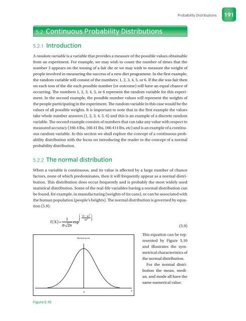
the human population (people’s heights). The normal distribution is governed by equation
(5.9):
Figure 5.10
1
f X
2π exp
( )
( ) =
σ
⎛
2
X − µ ⎞
⎜ − ⎟
2
⎝
⎜ 2σ
⎠
⎟
Normal curve
µ
X
Probability Distributions
(5.9)
This equation can be represented
by Figure 5.10
and illustrates the symmetrical
characteristics of
the normal distribution.
For the normal distribution
the mean, median,
and mode all have the
same numerical value.
191