- Page 2 and 3:
Learning statistics with R: A tutor
- Page 4 and 5:
This book is published under a Crea
- Page 6 and 7:
Preface Table of Contents I Backgro
- Page 8 and 9:
8.6 Summary . . . . . . . . . . . .
- Page 10 and 11:
VI Endings, alternatives and prospe
- Page 12 and 13:
February 16, 2015 Preface to Versio
- Page 14 and 15:
and density is discussed. A detaile
- Page 17 and 18:
1. Why do we learn statistics? “T
- Page 19 and 20:
And finally, an invalid argument wi
- Page 21 and 22:
Admission rate (both genders) 0 20
- Page 23 and 24:
experiment, and they don’t get an
- Page 25 and 26:
2. A brief introduction to research
- Page 27 and 28:
different ways: the length of time
- Page 29 and 30:
that when I ask 100 people how they
- Page 31 and 32:
Table 2.1: The relationship between
- Page 33 and 34:
2.3 Assessing the reliability of a
- Page 35 and 36:
2.5.1 Experimental research The key
- Page 37 and 38:
things “inside” the study. Let
- Page 39 and 40:
they lack face validity, you’ll f
- Page 41 and 42:
that age is growing at an incredibl
- Page 43 and 44:
then it can be a big problem. 2.7.7
- Page 45 and 46:
2.7.10 Placebo effects The placebo
- Page 47 and 48:
it doesn’t, which one do you thin
- Page 49:
Part II. An introduction to R - 35
- Page 52 and 53:
go out into the real world. It’s
- Page 54 and 55:
download Rstudio. To understand why
- Page 56 and 57:
Most of this text is pretty uninter
- Page 58 and 59:
citation() To cite R in publication
- Page 60 and 61:
Table 3.1: Basic arithmetic operati
- Page 62 and 63:
Division / and Multiplication *, th
- Page 64 and 65:
sales * royalty [1] 2450 As far as
- Page 66 and 67:
x to the power of 0.5”. Personall
- Page 68 and 69:
As you can see, specifying the argu
- Page 70 and 71:
Figure 3.3: If you’ve typed the n
- Page 72 and 73:
sales.by.month sales.by.month [1]
- Page 74 and 75:
profit / days.per.month [1] 0.00000
- Page 76 and 77:
not true of R. R is not infinitely
- Page 78 and 79:
Table 3.3: Some more logical operat
- Page 80 and 81:
In other words, any.sales.this.mont
- Page 82 and 83:
and gotten exactly the same result.
- Page 84 and 85:
Figure 3.6: The options window in R
- Page 86 and 87:
- 72 -
- Page 88 and 89:
print( keeper ) [1] 8.539539 So, fr
- Page 90 and 91:
to import an SPSS data file into R,
- Page 92 and 93:
The output here is telling you that
- Page 94 and 95:
Figure 4.3: The Rstudio dialog box
- Page 96 and 97:
Figure 4.5: The Rstudio “Environm
- Page 98 and 99:
this should be obvious already. But
- Page 100 and 101:
Figure 4.6: The “file panel” is
- Page 102 and 103:
from this file into my workspace. T
- Page 104 and 105:
2 February 28 100 high 3 March 31 2
- Page 106 and 107:
Figure 4.9: The Rstudio window for
- Page 108 and 109:
4.6.1 Special values The first thin
- Page 110 and 111:
x y x * y Error in x * y : non-nu
- Page 112 and 113:
4.7.1 Introducing factors Suppose,
- Page 114 and 115:
factors in 7.11.2, but for now you
- Page 116 and 117:
An alternative method is to use the
- Page 118 and 119:
4.11 Generic functions There’s on
- Page 120 and 121:
load (base) R Documentation The R D
- Page 122 and 123:
Warning Saved R objects are binary
- Page 124 and 125:
- 110 -
- Page 127 and 128:
5. Descriptive statistics Any time
- Page 129 and 130:
mean of these observations is just:
- Page 131 and 132:
mean( afl.margins[1:5] ) [1] 36.6 A
- Page 133 and 134:
the median rises only to $62,500. I
- Page 135 and 136:
Next, let’s calculate means and m
- Page 137 and 138:
5.2 Measures of variability The sta
- Page 139 and 140:
English: which game value deviation
- Page 141 and 142:
and you get the same... no, wait...
- Page 143 and 144:
Mean − SD Mean Mean + SD Figure 5
- Page 145 and 146:
Negative Skew No Skew Positive Skew
- Page 147 and 148:
Platykurtic ("too flat") Mesokurtic
- Page 149 and 150:
e useful, let’s try this for a ne
- Page 151 and 152:
argument specifies the grouping var
- Page 153 and 154:
grumpiness score. 13 If the mean is
- Page 155 and 156:
Frequency 0 5 10 15 20 Frequency 0
- Page 157 and 158:
My grumpiness 40 50 60 70 80 90 4 6
- Page 159 and 160:
following extract illustrates the b
- Page 161 and 162:
Y1 4 5 6 7 8 9 10 Y2 3 4 5 6 7 8 9
- Page 163 and 164:
Okay, so let’s have a look at our
- Page 165 and 166:
pay 0.760 0.720 . 0.137 . 0.196 . d
- Page 167 and 168:
5 6.68 9.75 NA 5 6 5.99 5.04 72 6 B
- Page 169 and 170:
• Measures of variability. In con
- Page 171 and 172:
6. Drawing graphs Above all else sh
- Page 173 and 174:
delete the plot and then type a new
- Page 175 and 176:
Fibonacci 2 4 6 8 10 12 1 2 3 4 5 6
- Page 177 and 178:
high-level functions all rely on th
- Page 179 and 180:
type = ’p’ type = ’o’ type
- Page 181 and 182:
Fibonacci 2 4 6 8 10 12 1 2 3 4 5 6
- Page 183 and 184:
Figure 6.8: Altering the scale and
- Page 185 and 186:
y the height of the leftmost bar in
- Page 187 and 188:
6.3.1 Visual style of your histogra
- Page 189 and 190:
0 20 40 60 80 100 120 (a) (b) Figur
- Page 191 and 192:
0 20 40 60 80 100 120 Winning Margi
- Page 193 and 194:
0 50 100 150 200 250 300 Winning Ma
- Page 195 and 196:
6.5.3 Drawing multiple boxplots One
- Page 197 and 198:
Winning Margin 0 50 100 150 1987 19
- Page 199 and 200:
The second way do to it is to use a
- Page 201 and 202:
cor( x = parenthood ) # calculate c
- Page 203 and 204:
0 10 20 30 0 10 20 30 Adelaide Fitz
- Page 205 and 206:
value for mar is c(5.1, 4.1, 4.1, 2
- Page 207 and 208:
This takes the “active” figure
- Page 209 and 210:
7. Pragmatic matters The garden of
- Page 211 and 212:
in the command above I didn’t nam
- Page 213 and 214:
speaker ee onk oo pip makka-pakka 0
- Page 215 and 216:
2 7 3 3 1 3 3 -1 1 -1 BLAH BLAH BLA
- Page 217 and 218:
seen it before. In any case, those
- Page 219 and 220:
Table 7.2: Two more arithmetic oper
- Page 221 and 222:
fact R does provide a function for
- Page 223 and 224:
But suppose, on the other hand, tha
- Page 225 and 226:
is select several different variabl
- Page 227 and 228:
column number. So, if we want to pi
- Page 229 and 230:
case.2 upsy-daisy pip 2 case.4 makk
- Page 231 and 232:
Note that R will only allow you to
- Page 233 and 234:
7.6.2 Sorting a factor You can also
- Page 235 and 236:
Two other methods that I want to br
- Page 237 and 238:
At this point you should have two q
- Page 239 and 240:
(alcohol, caffeine or no drug). Bec
- Page 241 and 242:
3 3 female 4.6 643 7.4 226 7.3 412
- Page 243 and 244:
discuss melt() and cast() in a fair
- Page 245 and 246:
paste( hw, ng, sep = ".", collapse
- Page 247 and 248:
Table 7.3: The ordering of various
- Page 249 and 250:
Table 7.4: Standard escape characte
- Page 251 and 252:
sub( pattern = "a", replacement = "
- Page 253 and 254:
Figure 7.1: The booksales2.csv data
- Page 255 and 256:
note that if you don’t have the R
- Page 257 and 258:
etween the two. However, there are
- Page 259 and 260:
a third variable to the cross-tabs
- Page 261 and 262:
today print(today) # display the d
- Page 263 and 264:
encode numbers in binary, 29 0.1 is
- Page 265 and 266:
environment. And so when you type i
- Page 267 and 268:
8. Basic programming Machine dreams
- Page 269 and 270:
for ages, you figure out some reall
- Page 271 and 272:
Figure 8.2: A screenshot showing th
- Page 273 and 274:
8.1.5 Differences between scripts a
- Page 275 and 276:
to the second value in vector; and
- Page 277 and 278:
crunching, we tell R (on line 21) t
- Page 279 and 280:
What this does is create a function
- Page 281 and 282:
hundreds of other things besides. H
- Page 283:
Part IV. Statistical theory - 269 -
- Page 286 and 287:
me: I guess I don’t see that. Sur
- Page 288 and 289:
- 274 -
- Page 290 and 291:
discussion of probability theory is
- Page 292 and 293:
In this case 11 of these 20 coin fl
- Page 294 and 295:
frequentists do this sometimes. And
- Page 296 and 297:
Probability of event 0.0 0.1 0.2 0.
- Page 298 and 299:
proceed to roll all 20 dice, what
- Page 300 and 301:
(a) Probability 0.00 0.05 0.10 0.15
- Page 302 and 303:
In other words, there is a 76.9% ch
- Page 304 and 305:
Probability Density 0.0 0.1 0.2 0.3
- Page 306 and 307:
Shaded Area = 68.3% Shaded Area = 9
- Page 308 and 309:
Probability Density 0.0 0.1 0.2 0.3
- Page 310 and 311:
• The χ 2 distribution is anothe
- Page 312 and 313:
work rather than rchisq() - the obs
- Page 314 and 315:
- 300 -
- Page 316 and 317:
10.1.1 Defining a population A samp
- Page 318 and 319:
Figure 10.2: Biased sampling withou
- Page 320 and 321:
a stratified sampling technique you
- Page 322 and 323:
10.2 The law of large numbers In th
- Page 324 and 325:
Table 10.1: Ten replications of the
- Page 326 and 327:
Sample Size = 1 Sample Size = 2 Sam
- Page 328 and 329:
Sample Size = 1 Sample Size = 2 0.0
- Page 330 and 331:
efer to them. For instance, if true
- Page 332 and 333:
Average Sample Mean 96 98 100 102 1
- Page 334 and 335:
10.5 Estimating a confidence interv
- Page 336 and 337:
sense idea of what it means to say
- Page 338 and 339:
Average Attendance 0 10000 30000 19
- Page 340 and 341:
Here’s how to plot the means and
- Page 342 and 343:
Let’s suppose that this glorious
- Page 344 and 345:
Dan’s research hypothesis: “ESP
- Page 346 and 347:
the type I error rate. As Blackston
- Page 348 and 349:
Critical Regions for a Two−Sided
- Page 350 and 351:
Critical Region for a One−Sided T
- Page 352 and 353:
one based on Neyman’s approach to
- Page 354 and 355:
alternative hypothesis is a near ce
- Page 356 and 357:
Sampling Distribution for X if θ=.
- Page 358 and 359:
Table 11.2: A crude guide to unders
- Page 360 and 361:
ureaucratic process. It’s not par
- Page 362 and 363:
(binomial test was non significant)
- Page 365 and 366:
12. Categorical data analysis Now t
- Page 367 and 368:
observations that fall within the i
- Page 369 and 370:
it is when it predicts too many (wh
- Page 371 and 372:
df = 3 df = 4 df = 5 0 2 4 6 8 10 V
- Page 373 and 374:
That’s why I told R to use the up
- Page 375 and 376:
clubs 35 40 0.2 diamonds 51 60 0.3
- Page 377 and 378:
only one of many (albeit one of the
- Page 379 and 380:
That’s more or less what we’re
- Page 381 and 382:
Well, since these probabilities hav
- Page 383 and 384:
Chapek 9 has an unfortunate tendenc
- Page 385 and 386:
12.5 Assumptions of the test(s) All
- Page 387 and 388:
To get the test of independence, al
- Page 389 and 390:
This is a bit more output than we g
- Page 391 and 392:
subj.1 : 1 no :70 no :90 subj.10 :
- Page 393 and 394:
13. Comparing two means In the prev
- Page 395 and 396:
40 50 60 70 80 90 Grades Figure 13.
- Page 397 and 398:
Two Sided Test One Sided Test −1.
- Page 399 and 400:
lower.area print( lower.area ) [1]
- Page 401 and 402:
df = 2 df = 10 −4 −2 0 2 4 valu
- Page 403 and 404:
than I’ve done here. For instance
- Page 405 and 406:
Anastasia’s students Bernadette
- Page 407 and 408:
null hypothesis μ alternative hypo
- Page 409 and 410:
ut once again I’m going to start
- Page 411 and 412:
for the difference “(mean 1) minu
- Page 413 and 414:
null hypothesis μ alternative hypo
- Page 415 and 416:
13.5.1 The data The data set that w
- Page 417 and 418:
ciMean( x = chico$improvement ) 2.5
- Page 419 and 420:
Paired samples t-test Variables: gr
- Page 421 and 422:
Grouping variable: ID variable: tim
- Page 423 and 424:
In a one-sided confidence interval,
- Page 425 and 426:
are different tests. Secondly, I wa
- Page 427 and 428:
Table 13.1: A (very) rough guide to
- Page 429 and 430:
ut you no longer believe that the c
- Page 431 and 432:
Frequency 0 5 10 15 20 Normally Dis
- Page 433 and 434:
Sampling distribution of W (for nor
- Page 435 and 436:
We then count up the number of chec
- Page 437 and 438:
• A paired samples t-test is used
- Page 439 and 440:
14. Comparing several means (one-wa
- Page 441 and 442:
Mood Gain 0.5 1.0 1.5 placebo anxif
- Page 443 and 444:
This formula looks pretty much iden
- Page 445 and 446:
is true, then you’d expect all th
- Page 447 and 448:
mean square, MS w , can be viewed a
- Page 449 and 450:
3 placebo 0.1 0.45 -0.350 0.1225 4
- Page 451 and 452:
is choose an α level (i.e., accept
- Page 453 and 454:
names( my.anova ) [1] "coefficients
- Page 455 and 456:
etaSquared( x = my.anova ) eta.sq e
- Page 457 and 458:
One thing that bugs me slightly abo
- Page 459 and 460:
If we compare these three p-values
- Page 461 and 462: • Homogeneity of variance. Notice
- Page 463 and 464: Secondly, I did mention that it’s
- Page 465 and 466: Frequency 0 1 2 3 4 5 6 7 Sample Qu
- Page 467 and 468: Looking at this table, notice that
- Page 469 and 470: • Post hoc analysis and correctio
- Page 471 and 472: 15. Linear regression The goal in t
- Page 473 and 474: The Best Fitting Regression Line No
- Page 475 and 476: • data. The data frame containing
- Page 477 and 478: Figure 15.4: A 3D visualisation of
- Page 479 and 480: Wonderful. A big number that doesn
- Page 481 and 482: If our regression model has K predi
- Page 483 and 484: You can see why this is handy, sinc
- Page 485 and 486: what it is. The test for the signif
- Page 487 and 488: Fortunately, confidence intervals f
- Page 489 and 490: • Uncorrelated predictors. The id
- Page 491 and 492: Outlier Outcome Predictor Figure 15
- Page 493 and 494: Outcome High influence Predictor Fi
- Page 495 and 496: Cook’s distance 0.00 0.02 0.04 0.
- Page 497 and 498: Standardized residuals −2 −1 0
- Page 499 and 500: 78 Residuals vs Fitted Residuals
- Page 501 and 502: In a lot of cases, the solution to
- Page 503 and 504: Signif. codes: 0 *** 0.001 ** 0.01
- Page 505 and 506: 15.10.1 Backward elimination Okay,
- Page 507 and 508: + day 1 1.55760 1837.2 297.08 + bab
- Page 509 and 510: etween those two SS values as a sum
- Page 511: 16. Factorial ANOVA Over the course
- Page 515 and 516: drug 2 3.45 1.727 18.6 8.6e-05 ***
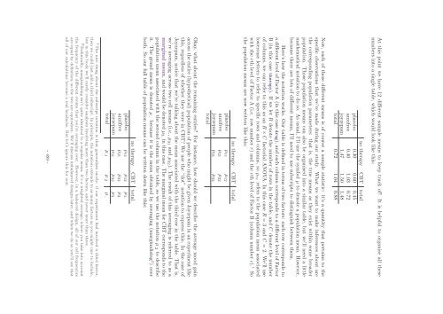
- Page 517 and 518: means can be organised into the sam
- Page 519 and 520: attributable to the “ANOVA model
- Page 521 and 522: Only Factor A has an effect Only Fa
- Page 523 and 524: The effect of CBT (difference betwe
- Page 525 and 526: Now, if you go back to the formulas
- Page 527 and 528: Here’s what I mean. Again, let’
- Page 529 and 530: Speaking of interaction effects, he
- Page 531 and 532: 16.4 Assumption checking As with on
- Page 533 and 534: 16.5.1 The F test comparing two mod
- Page 535 and 536: the degrees of freedom here is 15.
- Page 537 and 538: tfm.2 grade attend reading 1 90 yes
- Page 539 and 540: line, we obtain the following: Ŷ 7
- Page 541 and 542: Estimate Std. Error t value Pr(>|t|
- Page 543 and 544: that contains the same data as clin
- Page 545 and 546: What about the case when there does
- Page 547 and 548: R comes with a variety of functions
- Page 549 and 550: enlightening read. There are a lot
- Page 551 and 552: 16.8 Post hoc tests Time to switch
- Page 553 and 554: diff lwr upr p adj anxifree:no.ther
- Page 555 and 556: 1 yes none 3.700 2 no none 5.550 3
- Page 557 and 558: Analysis of Variance Table Response
- Page 559 and 560: III tests (which are simple) before
- Page 561 and 562: sugar 2.13 2 4.0446 0.045426 * milk
- Page 563 and 564:
even simpler. The main effect of su
- Page 565 and 566:
However, when we do the same thing
- Page 567:
Part VI. Endings, alternatives and
- Page 570 and 571:
first I want to work through a simp
- Page 572 and 573:
This is a very useful table, so it
- Page 574 and 575:
P pd|hqP phq P ph|dq “ P pdq And
- Page 576 and 577:
Bayesian approach relative to the o
- Page 578 and 579:
hardly unusual: in my experience, m
- Page 580 and 581:
Cumulative Probability of Type I Er
- Page 582 and 583:
are wrong. Worse yet, because we do
- Page 584 and 585:
library( BayesFactor ) # ...because
- Page 586 and 587:
make sense to people who already un
- Page 588 and 589:
-------------- [1] Non-indep. (a=1)
- Page 590 and 591:
Before moving on, it’s worth high
- Page 592 and 593:
17.6.2 The Bayesian version Okay, s
- Page 594 and 595:
[2] day : 0.2724027 ˘0% [3] baby.s
- Page 596 and 597:
therapy 0.4672 1 8.5816 0.01262 * d
- Page 598 and 599:
command that I use when I want to g
- Page 600 and 601:
- 586 -
- Page 602 and 603:
• Other types of correlations. In
- Page 604 and 605:
measurements mean that independence
- Page 606 and 607:
the list that I’ve given above is
- Page 608 and 609:
So if you were forced to guess my w
- Page 610 and 611:
to be able to do more than ANOVA, m
- Page 612 and 613:
Fisher, R. A. (1922a). On the inter