Lies, Damned Lies, or Statistics- How to Tell the Truth with Statistics, 2017a

40 3. LINEAR REGRESSION
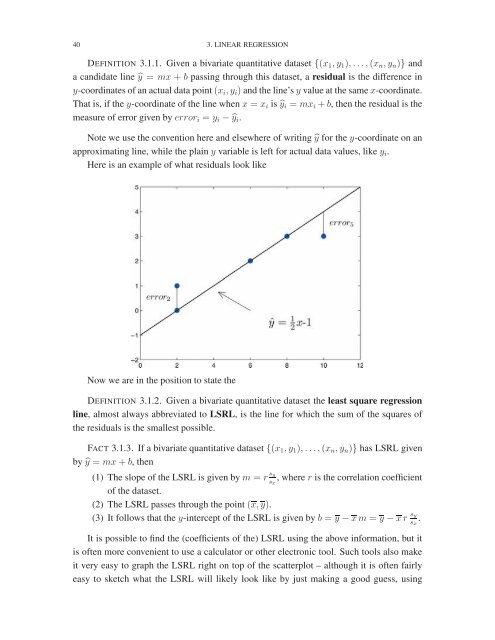
DEFINITION 3.1.1. Given a bivariate quantitative dataset {(x 1 ,y 1 ),...,(x n ,y n )} and
a candidate line ŷ = mx + b passing through this dataset, a residual is the difference in
y-coordinates of an actual data point (x i ,y i ) and the line’s y value at the same x-coordinate.
That is, if the y-coordinate of the line when x = x i is ŷ i = mx i + b, then the residual is the
measure of error given by error i = y i − ŷ i .
Note we use the convention here and elsewhere of writing ŷ for the y-coordinate on an
approximating line, while the plain y variable is left for actual data values, like y i .
Here is an example of what residuals look like
Now we are in the position to state the
DEFINITION 3.1.2. Given a bivariate quantitative dataset the least square regression
line, almost always abbreviated to LSRL, is the line for which the sum of the squares of
the residuals is the smallest possible.
FACT 3.1.3. If a bivariate quantitative dataset {(x 1 ,y 1 ),...,(x n ,y n )} has LSRL given
by ŷ = mx + b, then
(1) The slope of the LSRL is given by m = r sy
s x
,wherer is the correlation coefficient
of the dataset.
(2) The LSRL passes through the point (x, y).
(3) It follows that the y-intercept of the LSRL is given by b = y − xm= y − xr sy
s x
.
It is possible to find the (coefficients of the) LSRL using the above information, but it
is often more convenient to use a calculator or other electronic tool. Such tools also make
it very easy to graph the LSRL right on top of the scatterplot – although it is often fairly
easy to sketch what the LSRL will likely look like by just making a good guess, using