Proc. Neutrino Astrophysics - MPP Theory Group

arXiv:astro-ph/9801320v1 30 Jan 1998
Sonderforschungsbereich 375 • Research in Particle-Astrophysics
Technische Universität München (TUM) · Ludwig-Maximilians-Universität München (LMU)
Max-Planck-Institut für Physik (MPP) · Max-Planck-Institut für Astrophysik (MPA)
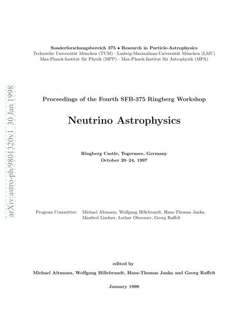
Proceedings of the Fourth SFB-375 Ringberg Workshop
Neutrino Astrophysics
Ringberg Castle, Tegernsee, Germany
October 20–24, 1997
Program Committee: Michael Altmann, Wolfgang Hillebrandt, Hans-Thomas Janka,
Manfred Lindner, Lothar Oberauer, Georg Raffelt
edited by
Michael Altmann, Wolfgang Hillebrandt, Hans-Thomas Janka and Georg Raffelt
January 1998

Proceedings of the Fourth SFB-375 Ringberg Workshop “Neutrino Astrophysics”
Sonderforschungsbereich 375 Research in Astro-Particle Physics
E-mail: depner@e15.physik.tu-muenchen.de
Postal Address:
Technische Universität München
Physik Department E15 — SFB–375
James-Franck-Straße
D–85747 Garching
Germany
c○ Sonderforschungsbereich 375 and individual contributors
Published by the Sonderforschungsbereich 375
Technische Universität München, D–85747 Garching
January 1998

Preface
This was the fourth workshop in our series of annual “retreats” of the Sonderforschungsbereich
Astroteilchenphysik (Special Research Center for Astroparticle Physics), or SFB for
short, to the Ringberg Castle above Lake Tegernsee in the foothills of the Alps. These
meetings are meant to bring together the members of the SFB which are dispersed between
four institutions in the Munich area, the Technical University Munich (TUM), the Ludwig-
Maximilians-University (LMU), and the Max-Planck-Institute for Physics (MPP) and that
for Astrophysics (MPA). We always invite a number of external speakers, including visitors
at our institutions, to complement the scientific program and to further the exchange of ideas
with the international community.
This year’s topic was “Neutrino Astrophysics” which undoubtedly is one of the central
pillars of astroparticle physics. We focused on the astrophysical and observational aspects
of this field, deliberately leaving out theoretical particle physics and laboratory experiments
from the agenda. Each day of the workshop was dedicated to a specific sub-topic, ranging
from solar, supernova and atmospheric neutrinos over high-energy cosmic rays to the early
universe. A session on future prospects served to conclude the workshop and provide an
outlook on the field in the next decade and beyond. We started every topical session with one
or two introductory talks, reviewing the status of theory and experiment and to providing
some background for the non-experts.
For the entire program we interpreted “neutrino astrophysics” in a broad sense, including,
for example, the physics of γ-ray bursts or the recent observations of TeV γ-rays by the
imaging air-Cherenkov technique. Some of the after-dinner-talks went significantly beyond a
narrow interpretation of the field! From our perspective the profile of neutrino astrophysics
as defined by our program worked very well, even better than we had hoped. We are proud
that the main complaint of the participants seemed to be that they did not get enough
mountain-hiking done because the sessions were too interesting to miss.
Besides regular SFB resources this workshop was made possible by a direct grant from
the Max-Planck-Society and additional funds from the Max-Planck-Institute for Astrophysics.
Special thanks go to the SFB secretary, Maria Depner, for her smooth and skillful management
of all practical matters related to the workshop.
We thank the participants for their high-level contributions and for being extremely cooperative
in submitting the “extended abstracts” of their talks on time and in a format that
allowed us to produce these proceedings in electronic form. Anyone interested in a printed
version should write to the SFB secretary at the address given on the previous page. We
hope that you will find this booklet a useful and up-to-date resource for the exciting and
fast-developing field of neutrino astrophysics.
Michael Altmann, Wolfgang Hillebrandt, Hans-Thomas Janka and Georg Raffelt
Munich, January 1998
iii

Contents
History
R.L. Mößbauer
History of Neutrino Physics: Pauli’s Letters ......................................... 3
A. Dar
What Killed the Dinosaurs? ........................................................ 6
Solar Neutrinos
M. Stix
Solar Models ...................................................................... 13
H. Schlattl, A. Weiss
Garching Solar Model: Present Status .............................................. 19
M. Altmann
Status of the Radiochemical Gallium Solar Neutrino Experiments .................. 22
Y. Fukuda (for the Superkamiokande Collaboration)
Solar Neutrino Observation with Superkamiokande ................................. 26
M.E. Moorhead (for the SNO Collaboration)
The Sudbury Neutrino Observatory ................................................ 31
L. Oberauer (for the Borexino Collaboration)
BOREXINO ....................................................................... 33
M. Junker (for the LUNA Collaboration)
Measurements of Low Energy Nuclear Cross Sections .............................. 36
G. Fiorentini
Solar Neutrinos: Where We Are and What Is Next? ............................... 40
Supernova Neutrinos
W. Hillebrandt
Phenomenology of Supernova Explosions ........................................... 47
B. Leibundgut
Supernova Rates ................................................................... 51
A.G. Lyne
Pulsar Velocities and Their Implications ........................................... 54
W. Keil
Convection in Newly Born Neutron Stars .......................................... 57
H.-Th. Janka
Anisotropic Supernovae, Magnetic Fields, and Neutron Star Kicks ................. 60
K. Sato, T. Totani, Y. Yoshii
Spectrum of the Supernova Relic Neutrino Background and Evolution of Galaxies .. 66
G.G. Raffelt
Supernova Neutrino Opacities ..................................................... 73
v

vi
S.J. Hardy
Quasilinear Diffusion of Neutrinos in Plasma ...................................... 75
P. Elmfors
Anisotropic Neutrino Propagation in a Magnetized Plasma ......................... 79
A.N. Ioannisian, G.G. Raffelt
Cherenkov Radiation by Massless Neutrinos in a Magnetic Field ................... 83
A. Kopf
Photon Dispersion in a Supernova Core ............................................ 86
Gamma-Ray Bursts
D.H. Hartmann, D.L. Band
Gamma-Ray Burst Observations ................................................... 91
S.E. Woosley, A. MacFadyen
Gamma-Ray Bursts: Models That Don’t Work and Some That Might ............... 96
M. Ruffert, H.-Th. Janka
Models of Coalescing Neutron Stars with Different Masses and Impact Parameters 101
R.A. Sunyaev
Physical Processes Near Black Holes .............................................. 106
High-Energy Neutrinos
K. Mannheim
Astrophysical Sources of High -Energy Neutrinos .................................. 109
P. Gondolo
Atmospheric Muons and Neutrinos Above 1TeV .................................. 112
D. Kie̷lczewska
Atmospheric Neutrinos in Super-Kamiokande ..................................... 116
Ch. Wiebusch
Neutrino Astronomy with AMANDA ............................................. 121
M.E. Moorhead
High Energy Neutrino Astronomy with ANTARES ................................ 127
R. Plaga
Ground-Based Observation of Gamma-Rays (200GeV–100TeV) .................. 130
Cosmology
C.J. Hogan
Helium Absorption and Cosmic Reionization ...................................... 139
K. Jedamzik
Non-Standard Big Bang Nucleosynthesis Scenarios ................................ 141
J.B. Rehm, K. Jedamzik
Big Bang Nucleosynthesis With Small-Scale Matter-Antimatter Domains .......... 147

M. Bartelmann
Neutrinos and Structure Formation in the Universe ............................... 149
Future Prospects
P. Meunier
Neutrino Experiments with Cryogenic Detectors .................................. 161
P.F. Smith
OMNIS—A Galactic Supernova Observatory ...................................... 165
J. Valle
Neutrinos in Astrophysics ........................................................ 170
L. Stodolsky
Some Neutrino Events of the 21st Century ........................................ 178
Appendix
Workshop Program and List of Participants ...................................... 183
Our Sonderforschungsbereich (SFB) “Astro-Teilchen-Physik” and its Divisions .... 193
vii

viii

History

History of Neutrino Physics: Pauli’s Letters
Rudolf L. Mößbauer
Physik Department E15, Technische Universität München, 85747 Garching, Germany
Editors’ Note
Professor Mößbauer gave an evening lecture on the history of neutrino physics during which
he read Pauli’s famous letters on the neutrino hypothesis. Rather than writing a formal contribution
to our proceedings, Professor Mößbauer suggested that we reproduce these letters.
(They were taken from Ref. [1] but can also be found in Ref. [2].) Because much of the
humour of Pauli’s writing is lost in the translation we quote the original German text. An
English translation can be found, for example, in Ref. [3].
Figure 1: Wolfgang Pauli (1900–1958) in Vienna 1933.
3

4
Pauli’s Letters
Brief an Oskar Klein, Stockholm, vom 18. 2. 1929
Aber ich verstehe zu wenig von Experimentalphysik um diese Ansicht beweisen zu können
und so ist Bohr in der für ihn angenehmen Lage, unter Ausnutzung meiner allgemeinen
Hilflosigkeit bei der Diskussion von Experimenten sich selber und mir unter Berufung auf
Cambridger Autoritäten (übrigens ohne Literaturangabe) da etwas beliebiges vormachen zu
können.
Brief an Oskar Klein, Stockholm, 1929
Ich selbst bin ziemlich sicher (Heisenberg nicht so unbedingt), daß γ-Strahlen die Ursache
des kontinuierlichen Spektrums der β-Strahlen sein müssen und daß Bohr mit seinen diesbezüglichen
Betrachtungen über eine Verletzung des Energiesatzes auf vollkommen falscher
Fährte ist. Auch glaube ich, daß die wärmemessenden Experimentatoren irgendwie dabei
mogeln und die γ-Strahlen ihnen nur infolge ihrer Ungeschicklichkeit bisher entgangen sind.
Brief an die Gruppe der “Radioaktiven” 1930
Physikalisches Institut
der Eidg. Technischen Hochschule
Zürich Zürich, 4. Dez. 1930
Liebe Radioaktive Damen und Herren!
Wie der Überbringer dieser Zeilen, den ich huldvollst anzuhören bitte, Ihnen des näheren aus-
einandersetzen wird, bin ich angesichts der falschen Statistik der N- und Li 6-Kerne, sowie des
kontinuierlichen β-Spektrums auf einen verzweifelten Ausweg verfallen, um den Wechselsatz
der Statistik 1 und den Energiesatz zu retten. Nämlich die Möglichkeit, es könnten elektrisch
neutrale Teilchen, die ich Neutronen 2 nennen will, in den Kernen existieren, welche den Spin
1/2 haben und das Ausschließungsprinzip befolgen und sich von Lichtquanten außerdem noch
dadurch unterscheiden, daß sie nicht mit Lichtgeschwindigkeit laufen. — Das kontinuierliche
β-Spektrum wäre dann verständlich unter der Annahme, daß beim β-Zerfall mit dem Elektron
jeweils noch ein Neutron emittiert wird, derart, daß die Summe der Energien von Neutron
und Elektron konstant ist.
Nun handelt es sich weiter darum, welche Kräfte auf die Neutronen wirken. Das wahrscheinlichste
Modell für das Neutron scheint mir aus wellenmechanischen Gründen dieses
zu sein, daß das ruhende Neutron ein magnetischer Dipol von einem gewissen Moment µ
ist. Die Experimente verlangen wohl, daß die ionisierende Wirkung eines solchen Neutrons
nicht größer sein kann als die eines γ-Strahls, und dann darf µ wohl nicht größer sein als
e · (10 −13 cm). Ich traue mich vorläufig aber nicht, etwas über diese Idee zu publizieren, und
wende mich erst vertrauensvoll an Euch, liebe Radioaktive, mit der Frage, wie es um den
experimentellen Nachweis eines solchen Neutrons stände, wenn dieses ein ebensolches oder
etwa 10mal größeres Durchdringungsvermögen besitzen würde wie ein γ-Strahl. ...
Also, liebe Radioaktive, prüfet, und richtet.—Leider kann ich nicht persönlich in Tübingen
erscheinen, da ich infolge eines in der Nacht vom 6. zum 7. Dez. in Zürich stattfindenden
Balles hier unabkömmlich bin. ... Euer untertänigster Diener W. Pauli
1 Heute Pauli’sches Ausschließungsprinzip
2 Heute Neutrinos

Brief an Oskar Klein, Stockholm, vom 12. 12. 1930
Ich kann mich vorläufig nicht entschließen, an ein Versagen des Energiesatzes ernstlich zu
glauben und zwar aus folgenden Gründen (von denen ich natürlich zugebe, daß sie nicht
absolut zwingend sind). Erstens scheint es mir daß der Erhaltungssatz für Energie-Impuls
dem für die Ladung doch sehr weitgehend analog ist und kann keinen theoretischen Grund
dafür sehen, warum letzterer noch gelten sollte (wie wir es ja empirisch über den β-Zerfall
wissen) wenn ersterer versagt. Zweitens müßte bei einer Verletzung des Energiesatzes auch
mit dem Gewicht etwas sehr merkwürdiges passieren.
Telegramm von Reines und Cowan vom 14. 6. 1957 an Wolfgang Pauli
We are happy to inform you that we have definitely detected neutrinos from fission fragments
by observing inverse beta decay of protons. Observed cross section agrees well with expected
6 · 10 −44 cm 2 .
References
[1] W. Pauli, Fünf Arbeiten zum Ausschließungsprinzip und zum Neutrino, Texte zur
Forschung Vol. 27 (Wissenschaftliche Buchgesellschaft Darmstadt, 1977).
[2] W. Pauli, Wissenschaftlicher Briefwechsel mit Bohr, Einstein, Heisenberg, u.a., Vol. II:
1930–1939, ed. by K. v. Meyenn, (Springer-Verlag, Berlin, 1985).
[3] W. Pauli, On the Earlier and More Recent History of the Neutrino (1957) in: Neutrino
Physics, ed. by K. Winter (Cambridge University Press, 1991).
5

6
What Killed The Dinosaurs?
Arnon Dar 1,2
1 Max-Planck-Institut für Physik (Werner-Heisenberg-Institut)
Föhringer Ring 6, 80805 München, Germany.
2 Department of Physics and Space Research Institute,
Technion, Israel Institute of Technology, Haifa 32000, Israel.
The early history of life during the Precambrian until its end 570 million years (My) ago
is poorly known. Since then the diversity of both marine and continental life has increased
exponentially. Analysis of fossil records shows that this diversification was interrupted by five
massive extinctions and some smaller extinction peaks [1]. The largest extinction occurred
about 251 My ago at the end of the Permian period. The global species extinction ranged then
between 80% to 95%, much more than, for instance, the Cretaceous-Tertiary extinction 64 My
ago which killed the dinosaurs and claimed ∼ 47% of existing genera [2]. In spite of intensive
studies it is still not known what caused the mass extinctions. Many extinction mechanisms
have been proposed but no single mechanism seems to provide a satisfactory explanation of
the complex geological records on mass extinctions [3]. These include terrestrial mechanisms
such as intense volcanism, which coincided only with two major extinctions [4] or drastic
changes in sea level, climate and environment that occurred too often, and astrophysical
mechanisms, such as a meteoritic impact that explains the iridium anomaly which was found at
the Cretaceous/Tertiary boundary [5] but has not been found in any of the other extinctions,
supernova explosions [6] and gamma ray bursts [7] which do not occur close enough at a
sufficiently high rate to explain the observed rate of mass extinctions.
The geological records, however, seem to indicate that an accidental combination of drastic
events [3] occurred around the times of the major extinctions. For instance, the dinosaur
extinction coincides in time with a large meteoritic impact, with a most intensive volcanic
eruption and with a drastic change in sea level and climate. The origin of these correlations is
still unclear. Meteoritic impacts alone or volcano eruptions alone or sea regression alone could
not have caused all the major mass extinctions. An impact of a 10 km wide meteorite with
a typical velocity of 30 km s −1 was invoked [5] in order to explain the Cretaceous-Tertiary
(K/T) mass extinction 64 My ago, which killed the dinosaurs, and the iridium anomaly
observed at the K/T boundary. But neither an iridium anomaly nor a large meteoritic
crater have been dated back to 251 My ago, the time of the Permian/Triassic (P/T) mass
extinction, which was the largest known extinction in the history of life [3] where the global
species extinction ranged between 80% to 95%. The gigantic Deccan volcanism in India that
occurred around the K/T boundary [4] and the gigantic Siberian basalts flood that occurred
around the P/T boundary have ejected approximately 2×10 6 km 3 of lava [4]. They were more
than a thousand times larger than any other known eruption on Earth, making it unlikely
that the other major mass extinctions, which are of a similar magnitude, were produced
by volcanic eruptions. Although there is no one-to-one correspondence between major mass
extinctions, large volcanic eruptions, large meteoritic impacts, and drastic environmental
changes, there are clear time correlations between them. We propose that near encounters
of Earth with “visiting planets” from the outer solar system are responsible for most of the
mass extinctions on planet Earth and can explain both the above correlations and the detailed
geological records on mass extinctions [8].

Recent observations with the Hubble Space Telescope of the Helix Nebula (Fig. 1) the
nearest planetary nebula, have discovered [9] that the central star is surrounded by a circumstellar
ring of about 3500 gigantic comet-like objects (“Cometary Knots”) with typical
masses about 10 −5 M⊙, comparable to our solar system planets (MEarth ≈ 3 × 10 −6 M⊙ and
MJupiter ≈ 9.6 × 10 −4 M⊙). It is not clear whether they contain a solid body or uncollapsed
gas. They are observed at distances comparable to our own Oort cloud of comets but they
seem to be distributed in a planar ring rather than in a spherical cloud like the Oort cloud.
It is possible that these Cometary Knots have been formed together with the central star
since star formation commonly involves formation of a thin planar disk of material possessing
too high an angular momentum to be drawn into the nascent star and a much thicker outer
ring of material extending out to several hundred AU. Evidence for this material has been
provided by infrared photometry of young stars and also by direct imaging.
It is possible that such Cometary Knots and the recently discovered gigantic asteroids [10]
in the outer solar system between the Kuiper belt and the Oort cloud are the high mass end
of the vastly more numerous low mass comets. The massive objects are more confined to
the ecliptic plane because of their relatively large masses, and form a circumstellar ring,
while the very light ones are scattered by gravitational collisions into a spherical Oort cloud.
Gravitational interactions in the ring can change their parking orbits into orbits which may
bring them into the inner solar system. In fact, various “anomalies” in the solar planetary
system [11] could have resulted from collisions or near encounters with such visitors in the
early solar system. These include [12] the formation of the moon, the large eccentricity and
inclination of some planetary orbits, the retrograde orbits of 6 moons of Jupiter, Uranus
and Neptune and the tilted spin planes of the Sun, the planets and moons relative to their
orbiting plane.
Strong gravitational tidal forces can cause frictional heating of planetary interiors leading
to strong volcanic activity, as seen, for instance, on Jupiter’s moon Io, the most volcanically
active object known in the solar system. The moon, the Sun and the known planets are too
far away to induce volcanic eruptions on Earth, but relatively recent “visits” of planet-like
objects near Earth could have generated gigantic tidal waves, large volcanic eruptions, drastic
changes in climate and sea level, and impacts of meteorites which were diverted into a collision
course with Earth by the passage through the astroids and Kuiper belts [13]. Thus, visiting
planets may provide a common origin for the diverse mass extinction patterns as documented
in the geological records.
Although exact calculations of surface tidal effects are a formidable scientific effort that
was begun by Newton and has continued and improved since then by many of the great mathematicians
and physicists, an approximate estimate of the flexing (h) of Earth (radius RE) by
a passing planet (distance d) can be easily obtained by neglecting the rotation of Earth and
the speed of the passing planet (mass Mp) and by assuming quasi hydrostatic equilibrium:
h ≈ 3
4
Mp
ME
� �3 RE
RE. (1)
d
The maximal crustal tide due to the moon is 27 cm. However, a visiting planet with a typical
mass like that of the Cometary Knots [9] which passes near Earth at a distance comparable
to the Earth-Moon distance produces gigantic oceanic and crustal tidal waves which are a
few hundred times higher than those induced by the moon. Oceanic tidal waves, more than
1 km high, can flood vast areas of continental land and devastate sea life and land life near
7

8
continental coasts. The spread of ocean waters by the giant tidal wave over vast areas of land
and near the polar caps will enhance glaciation and sea regression.
Flexing the Earth by h ∼ 100 m will deposit in it ∼ αGM2 Eh/R2 E ≈ 1034 ergs, where
α ∼ 0.1 is a geometrical factor. It is approximately the heat release within Earth during
106 y by radioactive decays. The flexing of Earth and the release of such a large energy in
a very short time upon contraction might have triggered the gigantic volcanic eruptions that
produced the Siberian basalts flood at the time of the P/T extinction and the Deccan basalts
flood at the time of the K/T extinction.
A reliable estimate of the masses and the flux of the visiting planets/planetesimals is not
possible yet. However, we have fixed them from the assumption that the unaccounted energy
source of Jupiter and its tilted spin plane relative to its orbital plane are both due to accretion
of visiting planets/moons. From the 3.13◦ tilt of Jupiter’s spin and the accretion rate, we
inferred that NJ ≈ 16 planets of average mass Mp ≈ 0.5ME have crashed into Jupiter during
its ∼ 4.57 Gy lifetime. Similar estimates for other planets, although yielding the correct order
of magnitude, are less reliable because the inferred number of accreted planets is too small.
The 7◦ tilt of the spin of the Sun could have been produced by the impact of ∼ 3 × 104 such
planets (ignoring possible angular momentum loss by the solar wind). This means that the
Sun has accreted ∼ 5% of its mass after its formation, at a rate of ∼ 7 planets per My. In
each capture episode, ∼ 6×1042 erg of gravitational energy is released in the Sun’s convective
layer. It produces optical and x-ray flashes at a rate ∼ 7 ×10−6 L −1
⊙ y−1 for Sun-like stars. It
also causes a significant luminosity rise for an extended time which may have induced climatic
and sea level changes on Earth, and extinctions of species which could not have adapted to
large environmental changes. The predicted rate is consistent with the observed rate of large
changes in O18 concentration in sea water sediments which record large changes in sea water
level and total glacier volume.
Using our inferred planet flux from Jupiter and its collimation by the Sun, we obtained that
a “visiting rate” of once every tv = 100 My for planets with Mp ∼ 0.5ME which fall towards
the Sun implies a passing distance of approximately 170,000 km from Earth which produces
crustal tidal waves of h ≥ 125 m and water tidal waves of ∼ 1 km height. The combination
of tidal waves, volcanic eruptions, meteoritic impacts and environmental and climatological
changes can explain quite naturally the biological and time patterns of mass extinctions. For
instance, the giant tidal waves devastate life in the upper oceans layers and on low lands
near coastal lines. They cover large land areas with sea water, spread marine life to dry on
land after water withdrawal, and sweep land life into the sea. They flood sweet water lakes
and rivers with salt water and erode the continental shores where most sea bed marine life
is concentrated. Amphibians, birds and inland species can probably survive the ocean tide.
This may explain their survival after the K/T extinction. Survival at high altitude inland
sites may explain the survival of some inland dinosaurs beyond the K/T border. Volcanic
eruptions block sunlight, deplete the ozone layer, and poison the atmosphere and the sea with
acid rain. Drastic sea level, climatic and environmental changes inflict further delayed blows
to marine and continental life. But high-land life in fresh water rivers which are fed by springs,
that is not so sensitive to temperature and climatic conditions, has better chances to survive
the tidal waves, the volcano poisoning of sea water, and the drastic sea level, environmental
and climatic changes.
Altogether, visiting planets offer a simple and testable solution to the puzzling correlations
between mass extinctions, meteoritic impacts, volcanic eruptions, sea regression and climatic
changes, as documented in the geological records. Perhaps the best test will come from the

MACHO sample of ∼100,000 light curves of variable stars: Planets/moons crashing onto stars
produce a big flash of light and soft x-rays from the hot spot at the impact point on main
sequence (rotating) stars, a nova-like thermonuclear explosion on the surface of a white dwarf
(rare), or a strong gamma ray flash from the surface of a neutron star (very rare).
Figure 1: A small section of a distant ring of gigantic comet-like objects around the central
star in the Helix nebula, the nearest planetary nebula, as seen recently by the Hubble Space
Telescope [9]. These objects have a typical mass of 5ME. Their gaseous heads have a typical
size of 10 15 cm. It is not clear whether they contain a solid body or uncollapsed gas.
Acknowledgements
It is a pleasure to thank the organizers of the workshop for their kind invitation and for an
excellent and enjoyable meeting. Very exciting and useful discussions with P. Gondolo, G.
Raffelt and L. Stodolsky during and after lunches at MPP, München, are greatfully acknowledged.
9

10
References
[1] M.J. Benton, Science 278, 52 (1995).
[2] C.B. Officer and J. Page, The Great Dinosaurs Controversy (Addison Wesley, 1996).
[3] D.H. Erwin, Nature 367, 231 (1994); Scientific American, July 1996, 56.
[4] V.A. Courtillot et al., Nature 333, 843 (1988); Scientific American, October 1990, 53.
[5] L.W. Alvarez et al., Science 208, 1095 (1980).
[6] R.A. Ruderman, Science 184, 1079 (1974).
[7] S.E. Thorsett, Ap. J. 444, L53 (1995). A. Dar, A. Laor, and N.J. Shaviv, astroph/9705006,
submitted to Phys. Rev. Lett. (1997).
[8] D. Fargion and A. Dar, “Tidal Effects of Visiting Planets”, submitted to Nature (1997).
[9] C.R. O’Dell and K. D. Handron, Astr. J. 111, 1630 (1996).
[10] J.A. Luu, Nature 387, 573 (1997).
[11] J. Audouze, J. and G. Israel, The Cambridge Atlas Of Astronomy (Cambridge Univ.
Press, 1985).
[12] J.W. Arnett, The Nine Planets, http://www.seds.org/nineplanets
[13] D.O. Whitemir and J.J. Matese, Nature 313, 36 (1986); P. Hut et al., Nature 329, 118
(1987).

Solar
Neutrinos

Solar Models
M. Stix
Kiepenheuer-Institut für Sonnenphysik, Freiburg, Germany
Introduction
A number of solar model calculations has been presented in recent years, especially in view of
the predicted flux of neutrinos from the Sun [4, 5, 6, 9, 12, 20, 27]. In the present contribution
I shall discuss mostly the Standard Solar Model. This model, including some refinements,
is confirmed by seismological tests. Non-standard models, on the other hand, face severe
difficulties. I close with a remark on the Sun’s magnetic field in the neutrino context.
The Standard Model
The standard solar model is a gas sphere in hydrostatic equilibrium. This may seem trivial.
However, some of the earliest non-standard models were based on the assumption of a very
strong internal magnetic field, or of rapid rotation of the solar core; both of these assumptions
violate the spherical symmetry as well as the hydrostatic equilibrium.
The input to the standard model should be to the best of our present knowledge. Let me
begin with the mass, luminosity, and radius,
m⊙ = (1.989±0.001)·10 30 kg , L⊙ = (3.845±0.008)·10 26 W , r⊙ = (6.960±0.001)·10 8 m .
The value given for the luminosity is from the ACRIM experiment on the Solar Maximum
Mission, with the error as quoted in [15]. The radius is for the optical depth τ = 2/3 where
the temperature is equal to the effective temperature (L⊙/4πσr 2 ⊙ )1/4 .
The age of the Sun is found by measuring the decay of long-lived radioactive isotopes in
meteorites,
t⊙ = (4.57 ± 0.05) · 10 9 years .
Wasserburg, in an appendix to [5], gives an even smaller error; the main source of uncertainty
is the not well-known state of the formation of the Sun at the time of the melting and
crystallization of the meteoritic material.
a) Chemical Composition
The composition of the solar surface (and the entire perfectly mixed outer convection zone) is
derived from solar spectroscopy and from meteoritic data. Recent results [16] show a slightly
decreased content of the heavy elements in comparison to earlier results, e.g. [1]. For oxygen,
the most abundant element after H and He, the change is −0.06 in the usual logarithmic
scale, or ≈ −13%. Altogether, the ratio of the mass fractions Z and X of the heavy elements
and hydrogen is 0.0245, instead of the earlier value 0.0267.
For helium the most accurate determination is based on helioseismology. This is because
both the sound velocity and the acoustic cut-off frequency depend on the adiabatic expo-
nent Γ1:
c 2 = PΓ1
ρ
, ωA = gΓ1
2c , Γ1
� �
dln T
=
dln P S
.
13

14
In the depth range where an abundant element is partly ionized Γ1 is greatly affected by the
energy of ionization. Thus the He abundance, in particular by its effect in the zone of partial
HeII ionization, has some influence on the eigenfrequencies of the Sun’s pressure (p) modes
of oscillation. The inversion of observed frequencies yields a mass fraction YS = 0.242 ±0.003
([22], other authors find similar results). It should be noted that the original He abundance,
Y0, is adjusted so that the luminosity of the present model, at age t⊙, equals L⊙. The result
of this procedure is Y0 = 0.27... 0.28, depending on other input to the model. The difference
to the seismically determined YS is appropriate in view of helium settling in the radiative
solar interior, see below.
b) Nuclear Reactions
Concerning the nuclear reactions I shall concentrate on the pp chains, which provide ≈ 99% of
the energy. The reaction rates, and therefore the branching between the three chains leading
to helium, depend on temperature (see below), and on the “astrophysical S-factor” S(E).
This factor depends weakly on the center-of-mass energy E and measures the cross section
after separation of 1/E times the penetration probability through the Coulomb barrier. For
the most important reactions Parker [21] reviews results of S-factors (at zero energy):
p(p,e + ν)d S11(0) = 3.89 · 10 −25 MeV·b ±1%
3 He( 3 He,2p) 4 He S33(0) = 5.0 MeV·b ±6%
3 He( 4 He,γ) 7 Be S34(0) = 533 eV·b ±4%
7 Be(p,γ) 8 B S17(0) = 22.2 eV·b ±14%
It is difficult to assess the errors. S11 is so small that it can only be calculated. The other
S-factors are measured in the laboratory but must be extrapolated to zero energy, and a
correction must be applied for electron screening at low energy. In particular the 14% error
of S17 has been criticized, e.g. [17], as it is derived from diverse experiments with partially
contradicting results in the range 17.9–27.7 eV·b. Perhaps better results will soon become
available as the measurements are extended to lower energy, cf. the contribution of M. Junker
to these proceedings.
c) Equation of State and Opacity
It is appropriate to discuss these two important ingredients to the solar model together, since
both depend on the knowledge of the number densities of the diverse particles, and especially
on the ionization equilibria and the electron density. To first order the Sun consists of a
perfect gas; but significant corrections, at the percent level, arise e.g. from the electrostatic
interaction of the particles (especially at the depth where abundant species are partially
ionized) and from partial electron degeneracy (in the core), cf. [23]. Modern standard models
are usually calculated with a tabulated equation of state and opacity. The most recent tables
from the Lawrence Livermore Laboratory [18] still exhibit unexplained discrepancies of up to
20% as compared to various other calculations; in the energy-generating region of the Sun
the uncertainty probably is much less, 2.5% according to [4].
Generally, the recent opacities [18] are somewhat increased in comparison to earlier results,
e.g. from Los Alamos, mainly because more elements have been included in the calculations.
The increase renders the radiative transport of energy less effective. The solar model responds
with a slightly raised central temperature (cf. discussion below), and a slightly lowered base of

the outer convection zone. As for the depth of the convection zone, there are two other input
modifications that may lead to an increase: convective overshoot (see below) and element
diffusion.
d) Element Diffusion
Driven by the gradients of pressure, temperature, and composition, helium and the heavy
elements diffuse toward the solar center, while hydrogen diffuses upward. The process is
slow, with a characteristic time exceeding the Sun’s age by a factor 100 or more. Nevertheless
diffusion should be included into the standard solar model since it produces significant effects,
especially in view of the details that can be seen by helioseismology. The following table
summarizes some results [5]:
Diffusion Y0 YS rb/r⊙ Tc(10 6 ) K snu(Cl) snu(Ga)
— 0.268 0.268 0.726 15.56 7.0 126
He 0.270 0.239 0.710 15.70 8.1 130
He & heavy el. 0.278 0.247 0.712 15.84 9.3 137
The obvious effect of a decreased surface mass fraction YS of He is essentially in agreement with
the results of other authors, and with the helioseismological result (see above); the increase of
YS obtained if heavy element diffusion is included is due to the larger initial helium content,
Y0, which is required in this case for the luminosity adjustment. Also, the central temperature
rises: Helium diffusion changes the mean molecular weight, which must be compensated by a
higher temperature in order to maintain the hydrostatic equilibrium; heavy element diffusion
increases the opacity, which must be compensated by a steeper temperature gradient (and
hence larger Tc) to maintain the radiative transport of energy. Together with Tc, the neutrino
rates predicted for the chlorine and gallium experiments are increased, as listed in columns
6 and 7 of the table. It should be noted that the Tc effect found in other calculations is
somewhat smaller, cf. the contribution of Schlattl and Weiss to these proceedings. Also, the
effect of helium diffusion on the depth of the convection zone (column 4) is in contrast to the
result of Cox et al. [12].
The depth of the convection zone has been determined from helioseismology by several authors.
Below the convection zone the temperature gradient is determined by the requirement
of radiative energy transport; within the convection zone the gradient is nearly adiabatic because
of the large heat capacity and hence large effectivity of the convective transport. Thus,
a prominent transition occurs in dT/dr and, accordingly, in dc 2 /dr. As the sound speed c(r)
can be obtained from the p-mode frequencies, the transition can be located. Christensen-
Dalsgaard et al. [10] find rb/r⊙ = 0.713±0.003, a more recent study [7] yields an even smaller
uncertainty, 0.713 ± 0.001, with the claim that systematic errors are included! — The temperature
at the base of the convection zone slightly depends on the helium abundance; for
the value of YS quoted above a good estimate [10] is (2.22 ± 0.05) · 10 6 K.
Neutrinos
The standard model of the Sun predicts the flux of neutrinos, as a function of neutrino energy,
that should be observed on Earth. So far 5 detectors have been used for such observations:
One using chlorine, two using gallium and two using water. The detectors as well as the
observational results are reviewed elsewhere in these proceedings. Briefly the results are
15

16
as follows: (1) All the detectors measure a significant neutrino flux, and so confirm that
nuclear energy generation actually takes place in the Sun. (2) The results of the two gallium
experiments agree with each other, and the results of the two water experiments agree with
each other. (3) All experiments measure a flux that lies significantly below the prediction of
the standard solar model. (4) The deficit depends on neutrino energy. This last point is of
particular interest for the solar model builder, because it is for this reason that it appears to
be impossible to repair all the deficits simultaneously by modifications of the solar model.
The significance of the neutrino deficit and its energy dependence has been illustrated by
a calculation of 1000 standard models [3] based on input parameters having normal distributions
with appropriate means and standard deviations. For the diverse neutrino experiments
these 1000 models predict results that have a certain spread but are clearly in conflict with
the actual measurements. If the predicted flux of energetic neutrinos originating from the
beta decay of 8 B is replaced by the value obtained in the water experiments (≈ 42% of the
predicted), then the predictions for the chlorine and gallium experiments become smaller
but are still significantly above the measurements. In other words, the existing experiments
cannot simultaneously be reconciled with the standard solar model.
In two recent calculations [13, 14] all the input parameters have been pushed to the extreme
in order to minimize the neutrino flux; nevertheless the prediction is still significantly too high.
Non-Standard Models
The aim of most non-standard solar models is to lower the temperature in the energygenerating
central region and thereby change the branching ratios of the three pp chains,
in particular in order to suppress a part of the high-energy 8 B neutrino flux. Castellani
et al. [9] discuss in detail the influence of the diverse input parameters on the central temperature
of the Sun. For example, a 45% increase of S11, or a 50% decrease of Z/X, or a 29%
decrease of the opacity would result in a 4% smaller central temperature. For the neutrino
fluxes resulting from 7 Be and 8 B the temperature dependence is [2]
Φν( 7 Be) ∝ T 8 c , Φν( 8 B) ∝ T 18
c .
Hence, a 4% cooler solar core reduces the predicted 8 B neutrino flux to 0.48 of the standard
value, and the flux of 7 Be neutrinos to 0.72. This may help to remove the discrepancy for the
water experiments, and to reduce the discrepancy for the chlorine experiment, but it provides
almost no help for the gallium experiments. Of the 137 snu (above table, last line) there
are only 16 from the decay of 8 B, but 38 from the electron capture of 7 Be. Thus a large
discrepancy remains; more specifically, the gallium experiments appear to leave no room for
the predicted 7 Be neutrinos. This is the major difficulty of the non-standard solar models.
Perhaps the neutrino discrepancy will finally be resolved by a combination of various
effects. A slight decrease of the central solar temperature Tc may be one of these effects,
although it is entirely unclear at present how such a decrease of Tc could be achieved. Heavy
element diffusion increases Tc, as we have seen. Mixing of the solar core apparently helps,
but the mixed-core model seems to fail the seismological test [28]. Other handles, such as
the opacity or the equation of state, permit only variations of Tc that are too small for a
substantial effect.
The conclusion is that most of the discrepancy should rather be resolved by non-standard
neutrinos. The energy-dependent conversion of electron neutrinos into other neutrino flavours
by the Mikeyev-Smirnov-Wolfenstein effect is a possibility; for a recent review see [17].

Convective Overshoot and Magnetism
Non-local versions of the mixing-length theory allow for overshooting flows at the base of
the solar convection zone [24, 25]. The overshoot layers calculated so far have a nearly adiabatic
temperature gradient. The thickness of such a layer should not exceed a few thousand
kilometers, according to helioseismological results [11]. On the other hand, some convective
overshoot will certainly occur and must be included into a calculation that is designed to
exactly reproduce the depth of the convection zone. The following table, adapted from [25],
gives a few examples of standard models, calculated without element diffusion. The input
consists of the opacity, the type of convection formalism (MLT: mixing-length theory, CM:
Canuto & Mazzitelli), equation of state (SS: Stix & Skaley [26], MHD: Mihalas et al. [19]),
initial helium mass fraction Y0, mixing-length parameter α. The results are the relative radius
rb/r⊙ where convection ceases, the central temperature Tc, and the predicted neutrino rates
for the Cl and Ga experiments. There is very little variation of these neutrino rates.
Nr Opacity MLT EOS Y0 α rb/r⊙ Tc6 snu (Cl) snu (Ga)
1 Alamos local SS 0.2733 2.403 0.7361 15.56 7.51 128.3
2 Alamos local MHD 0.2731 2.164 0.7325 15.55 7.49 128.2
3 Alamos nonl. SS 0.2733 2.409 0.7210 15.56 7.51 128.4
4 Alamos nonl. MHD 0.2732 2.168 0.7201 15.55 7.49 128.2
5 Opal92 local SS 0.2769 1.847 0.7231 15.56 7.68 129.4
6 Opal92 local MHD 0.2768 1.677 0.7194 15.56 7.66 129.3
7 Opal92 nonl. SS 0.2770 1.850 0.7114 15.57 7.68 129.4
8 Opal92 nonl. MHD 0.2768 1.679 0.7096 15.56 7.66 129.3
9 Opal95 local Opal95 0.2774 1.660 0.7220 15.59 7.81 130.0
10 Opal95 nonl. Opal95 0.2774 1.661 0.7116 15.59 7.81 130.0
11 Opal95 CM Opal95 0.2775 1.033 0.7218 15.58 7.80 129.9
12 Opal92 nonl. MHD 0.2768 1.680 0.7059 15.56 7.66 129.3
The overshoot layer appears especially attractive because it is the only place that can accommodate
a toroidal magnetic field of ≈ 10 5 G, suitable for the 11-year sunspot cycle. A similar
field strength is inferred from the latitude of field emergence at the Sun’s surface, as well as
from the tilt angle of bipolar spot groups with respect to the east-west direction [8]. With
10 5 G, and a layer thickness of, say, 5000 km, a neutrino should have a magnetic moment of
≈ 10 −10 µBohr in order to suffer a noticeable spin precession. This would be in conflict with
supernova SN1987A observations which indicate an upper limit of 10 −12 µBohr for the magnetic
moment of the neutrino. The reasoning may be even stronger as only a fraction of the
overshoot layer normally will be filled with magnetic flux. Matter-enhanced (resonant) spin
flip should also not occur since it requires an electron density exceeding that at the base of
the convection zone. Therefore, there appears to be no reason to speculate about a solar-cycle
dependence of the neutrino flux from the Sun.
References
[1] E. Anders and N. Grevesse, Geochim. Cosmochim. Acta 53 (1989) 197.
[2] J.N. Bahcall, Neutrino Astrophysics, Cambr. Univ. Press (1989).
17

18
[3] J.N. Bahcall and H.A. Bethe, Phys. Rev. D 47 (1993) 1298.
[4] J.N. Bahcall and M.H. Pinsonneault, Rev. Mod. Phys. 64 (1992) 885.
[5] J.N. Bahcall and M.H. Pinsonneault, Rev. Mod. Phys. 67 (1995) 781.
[6] A.B. Balantekin and J.N. Bahcall (Eds.), Solar Modeling, World Scientific (1995).
[7] S. Basu and H.M. Antia, Mon. Not. R. Astron. Soc. 287 (1997) 189.
[8] P. Caligari, F. Moreno Insertis, M. Schüssler, Astrophys. J. 441 (1995) 886.
[9] V. Castellani, S. Degl’Innocenti, G. Fiorentini, M. Lissia, B. Ricci, Phys. Rep. 281
(1997) 309.
[10] J. Christensen-Dalsgaard, D.O. Gough, M.J. Thompson, Astrophys. J. 378 (1991) 413.
[11] J. Christensen-Dalsgaard, M.J.P.F.G. Monteiro, M.J. Thompson, Mon. Not. R. Astron.
Soc. 276 (1995) 283.
[12] A.N. Cox, J.A. Guzik, R.B. Kidman, Astrophys. J. 342 (1989) 1187.
[13] A. Dar and G. Shaviv, Astrophys. J. 468 (1996) 933.
[14] H. Dzitko, S. Turck-Chièze, P. Delbourgo-Salvador, C. Lagrange, Astrophys. J. 447
(1995) 428.
[15] C. Fröhlich, P.V. Foukal, J.R. Hickey, H.S. Hudson, R.C. Willson, in C.P. Sonett, M.S. Giampapa,
M.S. Matthews (Eds.), The Sun in Time, Univ. Arizona (1991), p. 11.
[16] N. Grevesse, and A. Noels, in N. Prantzos, E. Vangioni-Flam, M. Cassé (Eds.), Origin
and Evolution of the Elements, Cambr. Univ. Press (1989), p. 15.
[17] N. Hata (1995), in [6], p. 63.
[18] C.A. Iglesias and F.J. Rogers, Astrophys. J. 464 (1996) 943.
[19] D. Mihalas, W. Däppen, D.G. Hummer, Astrophys. J. 331 (1988) 815.
[20] P. Morel, J. Provost, G. Berthomieu, Astron. Astrophys. 333 (1997) 444.
[21] P. Parker (1995), in [6], p. 25.
[22] F. Pérez Hernández and J. Christensen-Dalsgaard, Mon. Not. R. Astron. Soc. 269
(1994) 475.
[23] M. Stix, The Sun, Springer (1989).
[24] M. Stix, (1995) in [6], p. 171.
[25] M. Stix and M. Kiefer, in F.P. Pijpers, J. Christensen-Dalsgaard, J. Rosenthal (Eds.),
Solar convection and oscillations and their relationship, Kluver (1997), p. 69.
[26] M. Stix and D. Skaley, Astron. Astrophys. 232 (1990) 234.
[27] M. Takata and H. Shibahashi, Astrophys. J. (1998), submitted.
[28] R.K. Ulrich and E.J. Rhodes, Jr., Astrophys. J. 265 (1983) 551.

Garching Solar Model: Present Status
H. Schlattl, A. Weiss
Max-Planck-Institut für Astrophysik, Karl Schwarzschild-Str. 1, 85748 Garching, Germany
The Garching solar model code is designed to calculate high precision solar models. It allows
to control the numerical accuracy and has the best available input physics implemented [1].
It uses the OPAL-equation of state [2] and for the opacities those of [3] complemented by [4]
in the low-temperature regions. Pre-main sequence evolution is also taken into account. The
microscopic diffusion of hydrogen, helium, the isotopes participating in the CNO-cycle and
some additional metals (Ne, Mg, Si) is incorporated following the description of [5] for the
diffusion constants. The nuclear reaction rates were taken from [6].
In this work we want to emphasize the sensitivity of the structure of a solar model on the
interpolation technique used for the opacity tables. As the run of opacities (κ) with temperature
(T) and/or density (ρ) may show very rapidly changing gradients, choosing a suitable
interpolation procedure is not trivial. Our program uses two-dimensional bi-rational cubic
splines [7] to interpolate in the T-R-grid of the opacity tables (R = ρ/T 3 6 , T6 = T/10 6 K).
Apart from the general problem to choose suitable outer boundary conditions for the calculation
of the spline functions one can introduce an additional parameter to avoid artificial
unphysical oscillations, as they are typical in the case of cubic splines and rapidly varying
slopes. Increasing this damping parameter leads to almost linear interpolation just between
two grid points and to a very rapidly changing gradient at the grid points themselves. The
higher the damping parameter the more extended gets the linear region (a value of 0 corresponds
to standard cubic splines). The disadvantage of this damping is that in regions where
Figure 1: The run of κ and dlogκ/dlogR with R at fixed temperature of 2 million Kelvin
using pure cubic splines (dashed line) and damped cubic splines (full line). The arrows mark
the value of R at this temperature in a typical solar model.
19

20
the opacity has a very slowly changing gradient too high values for the damping parameter
lead to an interpolated run of opacity with T and/or R which shows step-like gradient variations.
This is illustrated in Fig. 1 where the full line shows the interpolated κ(R) using a
high damping parameter and the dashed line the run of κ without damping. In this case
a simple cubic spline seems to describe a better fit. The greatest deviations of κ between
two tabulated values is only about 3%, which is smaller than the quoted uncertainty for the
opacities of about 10%. We would like to note here that neither of the chosen interpolation
schemes can claim to reproduce the true values, as interpolation is always an estimation.
To illustrate the influence of the opacity interpolation, two solar models were calculated,
GARSOM3 with no and GARSOM2 with strong spline damping. The run of sound speed of
both models is compared with a seismic mode from [8] in Fig. 2. The deviation of GARSOM2
(dashed line) from the seismic model just below the convective zone is about twice as large
as compared with GARSOM3 (full line). At r = 0.67 R⊙ the temperature is approximately
2 million Kelvin, log10R ≈ −1.7. Regarding Fig. 1 one notices that at this radius the model
is in T-R-regions of the opacity tables where the different interpolations schemes differ most.
Figure 2: The run of quadratic sound speed of various models compared to seismic model
from [7]. Full line: GARSOM2, dashed line: GARSOM3, dotted line: reference model from
which the seismic model is inferred.
As the possible error in the tabulated opacities (10%) is bigger than the difference due to
interpolation (3%), neither of the models can be favoured from the theoretical point of view.
Although we must admit that κ(R,T) inferred from cubic splines without damping does look
more reliable, we can not really rule out GARSOM2. It is therefore necessary to improve the
grid density in the tables and the input physics in the opacities.
To show that GARSOM3 is compatible with solar models from other groups, we have
plotted in Fig. 2 also the run of sound speed of the reference model which was used to
infer the seismic model of [8]. The remaining discrepancies between the reference model and
GARSOM3 may be due to slightly different ages or nuclear reaction rates.

Acknowledgments
We would like to thank Jørgen Christensen-Dalsgaard who helped to detect the sensitivity
of opacity to interpolation. Additionally we acknowledge Sarbani Basu who provided us her
seismic model.
References
[1] H. Schlattl, A. Weiss and H.-G. Ludwig, A&A 322 (1997) 646.
[2] F.J. Rogers, F.J. Swenson and C.A. Iglesias, ApJ 456 (1996) 902.
[3] C.A. Iglesias and F.J. Rogers, ApJ 464 (1996) 943.
[4] D.R. Alexander and J.W. Fergusson, ApJ 437 (1994) 879.
[5] A.A. Thoul, J.N. Bahcall and A. Loeb, ApJ 421 (1994) 828.
[6] V. Castellani et al., Phys.Rev.D 50 (1994) 4749.
[7] H. Späth, Spline-Algorithmen zur Konstruktion glatter Kurven und Flächen, Oldenbourg,
München, 1973.
[8] S. Basu, Mon. Not. R. Astr. Soc. (1997) in press.
21

22
Status of the Radiochemical Gallium Solar Neutrino
Experiments
Michael Altmann
Physik Department E15, Technische Universität München, D–85747 Garching
and Sonderforschungsbereich 375 Astro-Particle Physics
With the successful completion of Gallex after six years of operation and the smooth transition
to Gno a milestone in radiochemical solar neutrino recording has been reached. The
results from Gallex, 77 ±6±5SNU, and Sage, 74 +11
−10 +5
−7 SNU, both being significantly below
all solar model predictions, confirm the long standing solar neutrino puzzle and constitute
an indication for non-standard neutrino properties. This conclusion is validated by the results
of 51Cr neutrino source experiments which have been performed by both collaborations and
71As doping tests done in Gallex.
GALLEX and SAGE: Radiochemical Solar Neutrino Recording
The radiochemical gallium detectors, Gallex and Sage, have been measuring the integral
solar neutrino flux exploiting the capture reaction 71 Ga + νe → 71 Ge + e − . The energy
threshold being only 233keV, this reaction allows to detect the pp-neutrinos from the initial
solar fusion step which contribute about 90% to the total solar neutrino flux.
In a typical run the target, consisting of 30tons of gallium in the form of 101t GaCl3
solution for Gallex and 55t of metallic gallium for Sage, is exposed to the solar neutrino
flux for 3-4 weeks. In the following I will mainly focus on Gallex, as for Gallex and Sage
the experimental procedure – apart from the chemical extraction of the neutrino produced
71 Ge and the stable germanium carrier which is added at the beginning of each run – is
rather similar. Both experiments use the signature provided by the Auger electrons and Xrays
associated with the decay 71 Ge + e − → 71 Ga + νe for identification of 71 Ge during a
several months counting time. Referring to [4, 5] for a detailed description of the detector
setup and experimental procedure I concisely summarize the Gallex experimental program
in table 1.
Table 1: GALLEX experimental program. It comprises 4 periods of solar neutrino observations
(Gallex 1 – Gallex 4), two chromium neutrino source experiments (Source I and Source II) and the
arsenic test.
date exposure period number of runs result
5/91–4/92 Gallex I 15 solar + 5 blank 81 ± 17 ± 9 SNU
8/92–6/94 Gallex II 24 solar + 22 blank 75 ± 10 +4
−5 SNU
6/94–10/94 Source I ( 51Cr) 11 source runs R = 1.01 +0.11
−0.10
10/94–10/95 Gallex III 14 solar + 4 blank 54 ± 11 ± 3 SNU
10/95–9/96 Source II ( 51Cr) 7 source runs R = 0.84 +0.12
−0.11
9/96–1/97 Gallex IV 12 solar + 5 blank 118 ± 19 ± 8 SNU
1/97–3/97 71As-test 4 arsenic runs Y = 1.00 ± 0.03

The combined result of all 65 Gallex solar runs is 76.4 ± 6.3 +4.5
−4.9 SNU. We note, however,
that for the Gallex-IV period pulse shape information is used only for K-peak signals. The
present result from Sage, 74 +11
−10 +5
−7 SNU [7], is in perfect agreement with Gallex.
The overall results from both experiments are only about 60% of the predictions from solar
model calculations, which constitutes an indication for non-standard neutrino properties, even
without considering the results from other solar neutrino experiments.
The 51 Cr neutrino source experiments
In order to validate this conclusion and check the reliability and efficiency of their detectors,
both collaborations have prepared intense (≈ 2MCi (Gallex) and 517kCi (Sage)) 51 Cr
neutrino sources by neutron irradiating isotopically enriched Cr [3]. 51 Cr decays by EC and
emits neutrinos of energy 750keV (decay to g.s., 90%) and 430keV (decay to 320keV excited
level, 10%), nicely accommodating the neutrino energies of the solar 7 Be branch.
For Gallex, the source has been inserted in the central tube of the target tank. Altogether
18 extractions have been performed with the source in place, divided into two series of
measurements with the source being re-activated in between. Figure 1 shows the individual
run results.
Figure 1: Individual run results of the GALLEX chromium neutrino source experiments,
normalized to the known source activity, as a function of time after the end of neutron
irradiation of the source. The horizontal bars indicate the durations of the exposures, the
exponential curve the expectation from the decay of the source. Source I and Source II runs
are represented by circles and diamonds, respectively.
An analysis of Source I and Source II yields R = 1.01 +0.11
+0.12
−0.10 and R = 0.84 −0.11 , respectively,
where R is the source activity as deduced from the neutrino measurement normalized to the
23

24
known true source activity. The combined analysis of both series results in R = 0.93 ± 0.08,
clearly demonstrating the absence of large systematic errors which could account for the
observed 40% solar neutrino deficit.
A similar experiment has also been performed by the Sage collaboration. They got a
quantitative recovery of R = 0.95 ± 0.12 [6].
The fact that both experiments, though employing different chemistry, demonstrated in
these experiments full efficiency, proves the trustworthiness of the radiochemical method and
shows that the 40% solar neutrino deficit observed in the radiochemical gallium experiments
cannot be ascribed to unknown systematic errors. In particular, the 51 Cr neutrino energies
nicely accommodating those from the solar 7 Be-branch, the full efficiency of the gallium
experiments to 7 Be-neutrinos is demonstrated.
71 As experiments
However, though the 51 Cr source in Gallex did outperform the sun by more than a factor
15 after insertion into the target tank, the experiments still are low statistics, involving only
several dozens of neutrino produced 71 Ge atoms. Therefore, at the very end of Gallex the
collaboration has performed a large-scale test of potential effects of hot chemistry, which
might lead to a different chemical behaviour of 71 Ge produced in a nuclear reaction compared
to the stable Ge carrier isotope: The in-situ production of 71 Ge by β−decay of 71 As. A known
quantity of 71 As (O(10 5 ) atoms) has been added to the tank (t-sample), where it decayed with
T 1/2 = 2.9d to 71 Ge. Four runs have been made under different operating conditions (mixing,
carrier addition, standing time), cf. table 2. For every spike a reference sample (e-sample)
was kept aside, making possible to calculate the ratio of t- and e-sample which does not suffer
from most of the systematic uncertainties associated with 71 Ge-counting.
Table 2: Experimental conditions and results (ratio t-sample/e-sample) of the 71 As runs.
run mixing conditions Ge-carrier standing result
[h × m 3 /h] addition time (tank / external)
A1 22 × 5.5 with As 19.9 d 1.01 ± 0.03
+0.17 × 60
A2 6 × 5.5 no Ge-carrier 19.9 d 1.00 ± 0.03
B3-1 24 × 5.5 after As 2.0 d 1.01 ± 0.03
B3-2 — after As 22.0 d 1.00 ± 0.03
In all cases a quantitative recovery of 100% was achieved. This demonstrates on a 3%-level the
absence of withholding effects even under unfavourable conditions like carrier-free operation 1 .
Gallium Neutrino Observatory
With the 71 As-tests Gallex has completed its large-scale experimental program. However,
solar neutrino measurements with a gallium target at Gran Sasso will be re-commenced in
spring 1998 in the frame of the Gallium Neutrino Observatory (GNO) [2] which is designed for
1 The stable germanium carrier is not only used for determination of the extraction yield, but also plays the
role of an ’insurance’ to saturate potential trace impurities which might capture 71 Ge in non-volatile complexes.

long-term operation covering at least one solar cycle. In its first phase GNO will use the 30ton
target of Gallex. However, for a second phase it is planned to increase the target mass to
60tons and later to 100tons. In addition, as it is equally important to decrease the systematic
uncertainty, effort is made to improve 71 Ge counting, both by improving the presently used
proportional counters, and by investigating novel techniques like semiconductor devices and
cryogenic detectors [1].
Acknowledgements
Our contribution to Gallex and Gno is supported by grants from the german BMBF, the
SFB-375, and the Beschleunigerlaboratorium Garching.
References
[1] M.Altmann et al., Development of cryogenic detectors for GNO, Proc. 4th Int. Solar
Neutrino Conf., ed.: W. Hampel, Heidelberg, Germany, 1997.
[2] E.Bellotti et al., Proposal for a permanent gallium neutrino observatory at Gran Sasso,
1996.
[3] M.Cribier et al., Nucl. Inst. Meth. A 378 (1996) 233.
[4] Gallex Collaboration, Phys.Lett. B 285 (1992) 376.
[5] E.Henrich et al., Angew. Chem. Int. Ed. Engl. 31 (1992) 1283.
[6] SAGE Collaboration, Phys. Rev. Lett. 77 (1996) 4708.
[7] SAGE Collaboration, in Proc. 4th Int. Solar Neutrino Conf., ed.: W. Hampel, Heidelberg,
Germany, 1997.
25

26
Solar Neutrino Observation with Superkamiokande
Yoshiyuki Fukuda (for the Superkamiokande Collaboration)
Institute Cosmic Ray Research, University of Tokyo, Japan
Introduction
Superkamiokande, which is a second generation solar neutrino experiment, is an imaging
water Cherenkov detector with 50,000 tons of pure water in the main tank. The detector is
located 1000 m underground (2700 m water equivalent) in Kamioka Zinc mine in the Gifu
prefecture of Japan, at 36.4 ◦ N, 137.3 ◦ E and 25.8 ◦ N geomagnetic latitude.
Figure 1: Schematic view of the Superkamiokande detector.
The detector consists of a main inner counter and an outer anti-counter. A schematic view
of the detector is shown in Fig. 1. The inner counter is contained in a cylindrical stainless-steel
tank and has a volume of 39.3 m in diameter × 42.0 m in height, containing 50,000 metric
tons of water. A total 11,146 photo multipliers (PMTs) with 20 inch φ photo cathode area
cover 40% of the entire inner surface of the tank. The fiducial mass for the solar neutrino
measurement is 22,500 tons, with boundaries 2.0 m from the inner surface. On the other
hand, a 4π solid-angle anti-counter surrounding the inner counter is also a water Čerenkov
counter of total mass 13,000 metric tons with 1850 PMTs to detect any signals coming from
outside of the detector and to shield against gamma-rays and neutrons.
Calibrations
The timing calibration for all PMTs is done by the Xe lamp. We usually take those data for
every 3 months and the maps of T-Q response for all PMTs are produced. This table is used
for correct timing as a function of observed charge in real data analysis.

The variation of the water transparency is obtained by stopping muon spectrum (Michael
spectrum). This is very important for obtaining the energy scale to be stable as a function
of time. The energy is almost proportional to the number of hitted PMTs, however, the
number maybe variable to the attenuation length of the water. Corrected number of hitted
PMTs is very stable to the variation of water transparency. This is also confirmed by the
γ-ray source which is emitted by the reaction of Ni(n,γ)Ni ∗ . The absolute values of water
transparency at various points of wavelength are measured by DYE-laser calibration. Recent
water transparency itself is very stable.
The performances of the detector, such as the absolute energy scale, the energy resolution,
the vertex resolution and the angular resolution are mainly calibrated by LINAC system. The
LINAC can generate an electron beam with 5 MeV to 16 MeV. This beam is induced via beam
pipe and bent by magnetic coil into the several positions of the tank. The typical values for
each resolution is 16%, 70cm and 22 degree for 10 MeV electrons. The absolute energy for
electron beam is calibrated by Ge solid state detector at each calibration time.
Monte Carlo simulation was tuned by the water transparency and other parameters to
reproduce the energy scale in various tank positions within 1% difference between MC and
real data.
Solar neutrino analysis
Superkamiokande has started from April 1996 and now processed about 400 days data for solar
neutrinos measurement. Analysis procedures are (1) noise reduction, (2) vertex reconstruction
and tight noise reduction, (3) spallation products cut, (4) fiducial volume (22.5 kton) cut and
(5) gamma ray cut. Some of analysis techniques are similar to Kamiokande’s ones, however,
most of them have been newly developed. In first step, we eliminate µ and decayed electron
and several electronics noise. The second step reconstructs the vertex using the timing of
hitted PMTs within selected 50 n second window. Main backgrounds in the residual data are
spallation products. In order to eliminate those events, we used the likelihood method using
the time difference and the distance between induced muon and those spallation events as
a function of muon energy. We can reject most of spallation products with 20% dead time.
In the last reduction, we reject external γ-rays coming from outside of the detector. Most
of those events are sitting at very close to the edge of fiducial volume and have an opposite
direction with respect to the detector wall. Event rate of the final sample is obtained by 175
events per day per 22.5 kton for 6.5 to 20 MeV.
From 1st May 1996 to 22 Oct 1997, we obtained 374.2 days data from Superkamiokande
measurement [1]. Figure 2 shows the angular distribution to the solar direction and the
heliograph for obtained final sample. In Fig. 2(a), best fit line which is expected by MC is
also shown. Extracted number of solar neutrinos is obtained by this fit as 4951 +117.9
−111.3 for 374.2
days data. Observed 8B solar neutrino flux is given by
or by taking ratio to the BP95 flux [3];
φ( 8 B) = 2.37 +0.06
−0.05 (stat.)+0.09
−0.07 (syst.) × 106 cm −2 sec −1
Data
SSMBP95
= 0.358 +0.009
−0.008 (stat.)+0.014
−0.010 (syst.).
The systematic error related to the energy scale has been reduced by LINAC calibration
and is obtained as 2.3%. Observed 8 B neutrino flux is significantly deficit to the expectation
of SSM(BP95) and it is consistent with the result from Kamiokande [2].
27

28
Events/day/kton/bin
0.3
0.25
0.2
0.15
0.1
0.05
SK 374day 6.5-20MeV 22.5kt ALL
0
-1 -0.5 0 0.5 1
cosθ sun
Figure 2: (a) Angular distribution to the solar direction and (b) heliograph for 374.2 days
data.
The energy spectrum of observed neutrinos is shown in Fig. 3(a). In this figure, expected
spectra of MSW small angle parameter and just-so parameter are also shown. At first sight,
small angle solution has better fit than flat (no oscillation) and just-so solution, but it is not
significant within an experimental error. The day and night flux difference is obtained by;
D − N
D + N
= −0.031 ± 0.024(stat.) ± 0.014(syst.).
If night data are divided into five bins, those differences are shown in Fig. 3(b). In this figure,
typical day/night flux variation of the large angle and the small angle solutions are also shown.
There is no significant difference in day/night fluxes in present observation. Also Fig. 3(c)
shows the seasonal variation of solar neutrino fluxes. Each season is pile up among different
years. Solid line corresponds to the expected variation from an eccentricity of the Sun orbit.
Within experimental error, there is no seasonal variation in present analysis. Those results
are also same ones from Kamiokande.
Two flavor neutrino oscillation
For astrophysical solution, it is generally difficult to explain the solar neutrino problem with
the modification of SSM including the observations from helioseismology. On the other hands,
the elementary particle solution using MSW neutrino oscillation [5] seems to be an excellent
for explanation of the solar neutrino problem, because it can distort the spectra of solar
neutrinos. Also MSW oscillation can give a effect in the day/night fluxes variation. As
obtained by Fig. 3, our observed spectrum can be seen slightly as distorted one, but not
seen in variance between day/night fluxes. Using these results, we can obtained the excluded
region at 95% C.L. in MS diagram as shown in Fig. 4(a).
If we take the constraint of measured 8 B solar neutrino flux, allowed region of 95%, 90%
and 68% C.L. as shown in Fig. 4(b). From these figures, our results and the allowed region
given by Ref. [4] are consistent in MSW oscillation analysis.

data/SSM BP95
1.2
1
0.8
0.6
0.4
0.2
0
7 8 9 10 11 12 13 14 15
MeV
8 B Solar Neutrino Flux (x10 6 /cm 2 /s)
4
3
2
1
0
JAN
data/SSM BP95
1
0.9
0.8
0.7
0.6
0.5
0.4
0.3
0.2
0.1
SK 374day 6.5-20MeV 22.5kt
FEB
MAR
APR
MAY
JUN
JUL
day
night1
night2
night3
night4
night5
0
-0.2 0 0.2 0.4 0.6 0.8 1
AUG
SEP
OCT
NOV
DEC
Figure 3: (a) Energy spectrum, (b) Day/Night flux variation and (c) seasonal variation of
obtained solar neutrino signal.
Summary
In summary, solar neutrino observation in Superkamiokande has started since May 1996 and
has already taken 374.2 days data. The observed 8 B solar neutrino flux is about 37% of the
prediction from SSM(BP95) and it is almost consistent with the result from Kamiokande.
Using LINAC calibration system, we can reduce the systematic errors related to the energy
scale. Obtained energy spectrum is likely distorted and it is indicated that the new physical
solution will be solved the solar neutrino problem. New challenge to lower threshold analysis
(≥ 5 MeV) has been started. Present radioactive ( 222 Rn) level is about 3 mBq/m 3 , however,
we will able to reduce that level to factor 1/5. Even though the present analysis, we have
succeeded to extract solar neutrino signals from 5–6.5 MeV region. Those data will give a
strong indication to the solution for the solar neutrino problem within a few years.
29

30
log(Δm 2 (eV 2 log(Δm ))
2 (eV 2 log(Δm ))
2 (eV 2 ))
-3
-4
-5
-6
-7
-8
-4 -3.5 -3 -2.5 -2 -1.5 -1 -0.5 0
log(sin 2 -8
-4 -3.5 -3 -2.5 -2 -1.5 -1 -0.5 0
log(sin 2θ)
2 day and night 5bins
-8
-4 -3.5 -3 -2.5 -2 -1.5 -1 -0.5 0
log(sin 2θ)
2 spectrum
2θ)
log(Δm 2 (eV 2 log(Δm ))
2 (eV 2 ))
-3
-4
-5
-6
-7
-8
-4 -3.5 -3 -2.5 -2 -1.5 -1 -0.5 0
log(sin 2 -8
-4 -3.5 -3 -2.5 -2 -1.5 -1 -0.5 0
log(sin 2θ)
2 day and night spectrum w/ flux constraint
2θ)
Figure 4: (a) 95% C.L. excluded region in MSW parameters. Inside of solid and dotted line
are excluded by the observed energy spectrum and the day/night flux difference, respectively.
(b) Allowed region in MSW parameters with measured 8 B neutrino flux. Thick solid line,
dashed line and thin solid line correspond to 95%, 90% and 68% C.L., respectively. Shaded
region is allowed at 95% C.L. by Hata.
References
[1] To be submitted.
[2] Y. Fukuda et al., Phys. Rev. Lett. 77, 1683 (1996).
[3] J.N. Bahcall and M. Pinsonneault, Rev. Mod. Phys. 67, 781 (1995).
[4] N. Hata and P. Langacker, IASSNS-AST 97/29, UPR-751T, hep-ph/9705339, May 1997.
[5] S.P. Mikheyev and A.Y. Smirnov, Sov. Jour. Nucl. Phys. 42, 913 (1985); L. Wolfenstein,
Phys. Rev. D17, 2369 (1978).

The Sudbury Neutrino Observatory
M.E. Moorhead (on behalf of the SNO Collaboration)
Particle and Nuclear Physics Laboratory, Keble Road, Oxford OX1 3RH, UK
The Sudbury Neutrino Observatory (SNO) [1] is a 1,000 ton heavy water (D2O) Cherenkov
detector in Sudbury, Ontario (Canada) which will start taking data in ‘98. The ν reactions
which occur in D2O and the extremely low background environment of the detector will allow
the following measurements: i) the νe and νx (flavour independent) fluxes, and their ratio,
for 8 B solar ν’s, ii) the energy spectrum of 8 B νe’s above 5 MeV, iii) time dependence in the
8 B flux, and iv) detailed studies of the ν burst from a galactic supernova, including a search
for νµ and ντ masses above 20 eV. For the 8 B solar ν measurements, the νe/νx flux ratio
and the νe energy spectrum constitute two separate tests of ν oscillations which are both
independent of solar model flux calculations [2]. If the currently favoured MSW solution [3]
of the solar neutrino problem is correct then the νe/νx flux ratio should provide conclusive
proof of oscillations with one year’s data yielding a 17 sigma departure from unity (statistical
error only).
The detector is situated two kilometers underground in a dedicated laboratory that has
been excavated in the Creighton nickel mine of INCO Corporation. This laboratory comprises
facilities for changing into clean-room clothing, a lunch room, a car wash for bringing
equipment into the clean area, a utility room where the H2O and D2O systems are located,
a control room and a 30 m × 23 m barrel shaped cavity for the detector itself. The walls
of the cavity have been coated with concrete and low-activity Urylon, a water proof radon
barrier. Inside this cavity is located a 12 m diameter spherical acrylic vessel (AV), recently
completed, for containing the D2O neutrino target. Almost completely surrounding this AV,
stands a 17 m geodesic sphere supporting 9,500 20-cm-Hamamatsu PMTs, each of which is
equipped with a light reflecting concentrator to increase its effective photocathode area by a
factor 1.7. Beginning in March ‘98, the detector will be filled with 7,000 tons of high purity
H2O outside the acrylic vessel (to act as shielding for high energy gamma rays coming from
the rock and the PMTs) and 1,000 tons of D2O inside the AV. The filling will take between
3–4 months and hence data taking will begin in mid-98.
The event rates for solar ν’s, assuming the full SSM 8 B flux [4], and for a supernova
(SN) at the center of our galaxy are given in Table 1. Apart from the neutral current (NC)
reaction, all of the events are detected by the array of 9,500 PMTs via the Cherenkov radiation
emitted by a single electron (or positron) of energy ≥ 5 MeV, the detector’s threshold. The
NC reaction produces a free neutron in the D2O which can be detected, after thermalization,
by observing a subsequent neutron capture reaction. There are three capture reactions of
interest depending on what additives are placed in the D2O:
i) Pure D2O: In the case of no additive there is a 30% probability of capture on deuterium,
which produces a 6.25 MeV gamma. This gamma converts to electrons by Compton scattering
and pair production, and the resulting Cherenkov light is detected by the PMTs. Five hundred
events a year are expected above the detector’s 5 MeV threshold.
ii) MgCl2: Dissolving 2 tons of MgCl2 in the D2O gives an 83% chance of neutron capture
on 35 Cl which produces an 8.5 MeV gamma cascade. The higher efficiency and Q-value of this
capture (c.f. capture on deuterium in the pure D2O case) increases the number of detected
events by a factor of 5 to 2,500 per year.
31

32
Table 1: Neutrino event rates in SNO (including detection efficiency). SSM refers to the event
rate per year for 8 B solar neutrinos assuming the standard solar model [4] and the small angle
MSW solution [3]. SN refers to a type II supernova at a distance of 10 kpc (the center of the
galaxy).
Neutrino reaction SSM SN
Charged Current (CC): νe + d → p + p + e − 3000 80
Neutral Current (NC): νx + d → p + n + νx 2500 300
Electron Scattering (ES): νe,x + e − → νe,x + e − 400 20
Anti-neutrino CC in D2O: ¯νe + d → n + n + e + 0 70
Anti-neutrino CC in H2O: ¯νe + p → n + e + 0 350
iii) 3 He Counters: An array of 3 He proportional counters [5] (5 cm diameter tubes of
800 m total length) placed vertically in the D2O in a square grid of 1m spacing, gives a 42%
chance of neutron capture on 3 He. The energy and rise-time of the signals are used to separate
n-capture (2,000 per year) from internal alpha and beta backgrounds.
The dominant background for all these NC detection methods will probably come from
photodisintegration of deuterium which produces free neutrons that are indistinguishable
from NC neutrons. Thus, the detector components have been carefully selected for extremely
low levels of thorium and uranium chain contamination so that the photodisintegration rate
is small compared with the NC rate. This small residual photodisintegration rate must
be measured, in order to subtract its contribution to the neutron capture signal. Several
methods have been developed for this purpose: i) radiochemical extraction and counting of
228 Th, 226 Ra, 224 Ra, 222 Rn and 212 Pb, ii) analysis of low energy signals seen by the PMT
array, iii) delayed coincidences between signals seen by the PMT array, and iv) prompt and
delayed coincidences between signals seen by the PMTs and signals in the 3 He proportional
counters.
References
[1] G.T. Ewan et al., Sudbury Neutrino Observatory Proposal, SNO 87-12 (1987).
[2] H.H. Chen, Phys. Rev. Lett. 55 (1985) 1534.
[3] N. Hata and P. Langacker, Phys. Rev. D 48 (1993) 2937.
[4] J.N. Bahcall and M.H. Pinsonneault, Rev. Mod. Phys. 64 (1994) 885.
[5] T.J. Bowles et al., Construction of an Array of Neutral-Current Detectors for the Sudbury
Neutrino Observatory, SNO internal report.

BOREXINO
L. Oberauer (for the Borexino Collaboration)
Technische Universität München, Physik Department E15, 85747 Garching, Germany
and Sonderforschungsbereich 375 Teilchen-Astrophysik
Physics Goals and Neutrino Detection with Borexino
The aim of the solar neutrino experiment Borexino is to measure in real time the solar
neutrino flux with low energy threshold at high statistics, and energy resolving via pure
leptonic neutrino electron scattering ν + e → ν + e.
Motivation for Borexino comes from the long standing solar neutrino puzzle. Data analysis
of the existing experiments leads to the assumption of severe suppression of the solar 7 Bebranch,
which probably cannot be explained by modifications of the standard astrophysical
model of the sun. The monoenergetic 7 Be-neutrinos give rise to a compton like recoil spectrum
in Borexino. Its edge will be at 660 keV, significantly higher than the aimed energy threshold
of ca. 250 keV. Thus 7 Be-neutrino detection is very efficient in Borexino.
Assuming validity of the standard model a counting rate for 7 Be-neutrinos, which would
consist in this case purely as νe, of roughly 55/day in Borexino is expected.
In scenarios of total neutrino flavour conversion (i.e. for neutrino mass differences ∆m 2 ≈
10 −6 −10 −5 eV 2 ) a reduced flux of approximately 12/day would be measured due to the lower
cross section of νµ,τ scattering, which occurs only via neutral current interaction.
In case of vacuum oscillations (i.e. for neutrino mass differences ∆m 2 ≈ 10 −10 eV 2 ) Borexino
would see a distinct time dependent periodical neutrino signal due to the seasonal eccentricity
of the earth’s orbit around the sun.
For neutrino mass differences in the range of ∆m 2 ≈ 10 −7 eV 2 and for large mixing
Borexino should see a ‘day/night’ effect due to electron neutrino regeneration during the
path through the earth.
Borexino also can serve for additional projects in neutrino physics. Search for a magnetic
moment can be performed by means of terrestrial neutrino sources by investigating the electron
recoil shape at low momentum transfer. Via the inverse beta-decay ¯νe + p → e + + n
Borexino can look for signals from geophysical neutrinos as well as for neutrinos emitted by
european nuclear power plants. The latter would serve as a long baseline neutrino oscillation
experiment probing the so-called large mixing angle solution for the solar neutrino problem.
The Detector and Background Considerations
The detector is shielded successively from outer radioactivity by means of an onion-like structure.
Here the adjacent inner layer serves as shielding and has to provide an increased purity
in terms of internal radioactivity.
Borexino is placed in hall C of the underground laboratory at Gran Sasso, Italy. An
overburden of ca. 3500 m.w.e. suppresses the cosmic muon flux to roughly 1/m 2 . The outer
part of the detector consists of a steel tank with 18 m in height and diameter. Inside this
‘external’ tank a stainless steel sphere will support 2200 phototubes on the inside and 200
tubes at the outside. Most of the tubes inside the sphere will be equipped with light guides in
order to increase the geometrical coverage and hence the energy resolution. Between external
33

34
tank and sphere high purity water will serve as shielding against external gamma rays and
as active Cherenkov counter against cosmic muons. The steel sphere will be filled with a
tranparent, high purity buffer liquid which itself holds a nylon sphere, filled with organic
scintillator. The active scintillator mass will be around 300 t. By means of time of flight
measurements event position can be reconstructed and a fiducial volume for solar neutrino
interaction defined. The latter should be about 100 t, establishing a counting rate of 55
neutrinos per day according to the standard solar model. The outer part of the scintillator
sphere serves as active shielding.
The demands on purity in terms of radioactivity in Borexino, especially for the scintillator
itself, are very severe. In order to be able to extract a clear signal from background events
also in case of total flavour conversion, an intrinsic concentration in Uranium and Thorium
of ca. 10 −16 should not be exceeded significantly. The amount of 14 C/ 12 C must not be higher
than ≈ 10 −18 . In order to test scintillating materials a large Counting Test Facility (CTF)
has been built up in hall C of the underground laboratory at Gran Sasso, which resembles to
a small prototyp (ca. 5 t of scintillator) of Borexino. From beginning of 1995 until summer
1997 several tests about the feasibilty of Borexino including procedures to maintain the purity
of the scintillator has been performed, which showed very encouraging results: 14 C/ 12 C =
1.85·10 −18 , 238 U = (3.5±1.3)·10 −16 g/g, 232 Th = (4.4±1.5)·10 −16 g/g. A complete discussion
of the CTF results including experimental techniques for further background suppression is
given in [1] and [2]. Details about the experimental setup of the CTF can be found in [3].
Highly developed neutron activation analysis of scintillation samples performed in Munich
is now sensitive in the same regime. For uranium an upper limit of 238 U < 2 ·10 −16 g/g (90%
CL) has been obtained. In addition concentration values or limits have been measured by
this method for a various amount of isotopes, including man-made nuclei. For details, see [4].
Background studies for Borexino include also the interaction of cosmic muons. The direct
detector response on muons has been determined by a coincidence measurement between the
CTF and a muon telescope on top of it. The time distribution of such events can be used
to discriminate between muon events and neutrino candidates at a level of 98%. However,
to reach the sensitivity needed to reach the goals in Borexino, the leak rate for muons must
not exceed a level of ≈ 10 −4 . Our design of the muon veto system therefore is threefold:
The outer region between external tank and steel sphere acts as Cherenkov counter, a special
configuration of the tubes inside the sphere will act as an additional muon identification
system, and finally the offline study of event topology like the time structure will help to
suppress this kind of background sufficiently.
Cosmogenic generation of radioactive nuclei has been sudied this fall at the 180 GeV muon
beam at SPS in CERN. Most dangerous source of events will come from 11 C-production in
the scintillator and surrounding buffer liquid. However, the energy spectrum of these events
is between 1 MeV and 2 MeV since the decay mode is positron decay at 1 MeV endpoint
energy. Thus the detection of 7 Be-neutrinos is not affected, however that of pep-neutrinos.
Prospects
Borexino is an international collaboration of about 60 scientists. Approved funding already
comes from INFN (Italy) and from BMBF and DFG (Germany). A substantial part should
also be covered by NSF (USA) in the near future. Work on the external tank of Borexino is
almost completed. We expect to finish with the inner steel sphere in 1999. Simultaneously
the CTF will be upgraded. Finally it will serve as test facility for Borexino scintillator

procurement in batch mode. Given full funding also for our american collaborators first data
taking may be expected at the end of the year 2000.
References
[1] G. Alimonti et al., BOREXINO collaboration, Astr. Phys. J. (1997), accepted for publication
[2] G. Alimonti et al., BOREXINO collaboration, Nucl. Phys. (1997), accepted for publication
[3] G. Alimonti et al., BOREXINO collaboration, Nucl. Instr. Meth. (1997), accepted for
publication
[4] T. Goldbrunner et al., Journ. of Rad. Nucl. Chem., 216, (1997) 293.
35

36
Measurements of Low Energy Nuclear Cross Sections
M. Junker (for the LUNA Collaboration)
Laboratori Nazionali Gran Sasso, Assergi (AQ), Italy
and Institut für Experimentalphysik III, Ruhr-Universität Bochum, Germany
The nuclear reactions of the pp-chain play a key role in the understanding of energy production,
nucleosynthesis and neutrino emission of the elements in stars and especially in our
sun [1]. A comparison of the observed solar neutrino fluxes measured by the experiments
GALLEX/SAGE, HOMESTAKE and KAMIOKANDE provides to date no unique picture
of the microscopic processes in the sun [2]. A solution of this so called “solar neutrino puzzle”
can possibly be found in the areas of neutrino physics, solar physics (models) or nuclear
physics. In view of the important conclusions on non-standard physics, which might be derived
from the results of the present and future solar neutrino experiments, it is essential to
determine the neutrino source power of the sun more reliably.
Due to the Coulomb Barrier involved in the nuclear fusion reactions, the cross section
of a nuclear reaction drops nearly exponentially at energies which are lower than the
Coulomb Barrier, leading to a low-energy limit of the feasible cross section measurements
in a laboratory at the earth surface. Since this energy limit is far above the thermal energy
region of the sun, the high energy data have to be extrapolated down to the energy
region of interest transforming the exponentially dropping cross section σ(E) to the
astrophysical S-factor S(E) = σ(E)E exp(2π η), with the Sommerfeld parameter given by
2π η = 31.29Z1 Z2(µ/E) 1/2 [1]. The quantities Z1 and Z2 are the nuclear charges of the interacting
particles in the entrance channel, µ is the reduced mass (in units of amu), and E
is the center-of-mass energy (in units of keV). In case of a non resonant reaction S(E) may
then be parameterized by the polynomial S(E) = S(0) + S ′ (0)E + 0.5S ′′ (0)E 2 .
As usual in physics, extrapolation of data into the “unknown” can lead onto “icy ground”.
Although experimental techniques have improved over the years to extend cross section measurements
to lower energies, it has not yet been possible to perform measurements within the
thermal energy region in stars.
For nuclear reactions studied in the laboratory, the target nuclei and the projectiles are
usually in the form of neutral atoms/molecules and ions, respectively. The electron clouds
surrounding the interacting nuclides act as a screening potential: the projectile effectively sees
a reduced Coulomb barrier. This leads to a higher cross section, σs(E), than would be the
case for bare nuclei, σb(E), with an exponential enhancement factor flab(E) = σs(E)/σb(E) ≃
exp(πη Ue/E) [3, 4] where Ue is the electron-screening potential energy (e.g. Ue ≃ Z1·Z2·e 2 /Ra
approximately, with Ra an atomic radius). For a stellar plasma the value of σb(E) must be
known because the screening in the plasma can be quite different from that in laboratory studies
[5], and σb(E) must be explicitly included in each situation. Thus, a good understanding
of electron-screening effects is needed to arrive at reliable σb(E) data at low energies. Lowenergy
studies of several fusion reactions involving light nuclides showed [6, 7, 8] indeed the
exponential enhancement of the cross section at low energies. The observed enhancement
(i.e. the value of Ue) was in all cases close to or higher than the adiabatic limit derived from
atomic-physics models. An exception are the 3 He+ 3 He data of Krauss et al. [10], which
show apparently no electron screening down to E=25 keV, although the effects of electron
screening should have enhanced the data at 25 keV by about a factor 1.2 for the adiabatic

limit Ue=240 eV. Thus, improved low-energy data are particularly desirable for this reaction.
The low-energy studies of thermonuclear reactions in a laboratory at the earth’s surface
are hampered predominantly by the effects of cosmic rays in the detectors. Passive shielding
around the detectors provides a reduction of gammas and neutrons from the environment,
but it produces at the same time an increase of gammas and neutrons due to the cosmicray
interactions in the shielding itself. A 4π active shielding can only partially reduce the
problem of cosmic-ray activation. The best solution is to install an accelerator facility [11] in
a laboratory deep underground [9]. The worldwide first underground accelerator facility has
been installed at the Laboratori Nazionali del Gran Sasso (LNGS) in Italy, based on a 50 kV
accelerator. This pilot project is called LUNA and has been supported since 1992 by INFN,
BMBF, DAAD-VIGONI and NSF/NATO.
The major aim of the LUNA project is to measure the cross section of 3 He( 3 He,2p) 4 He
which is one of the major sources of uncertainties for the calculation of the neutrino source
power. It has been studied previously [10] down to about Ecm=25 keV, but there remains the
possibility of a narrow resonance at lower energies that could enhance the rate of path I at
the expense of the alternative paths of the pp-chain that produce the high-energies neutrinos
(Eν > 0.8 MeV). The LUNA–facility allows to study this important reaction over the full
range of the solar Gamow Peak, where the cross section is as low as 8 pbarn at Ecm=25 keV
and about 20 fbarn at Ecm=17 keV.
Figure 1 shows the results obtained in the energy region between Ecm=25 keV and
Ecm=20.7 keV. The lowest counting rate was of 3 events per day at Ecm=20.7 keV. At
this energy about 1000 Cb of 3 He + have been accumulated on the target. The data obtained
at higher energies (450 kV accelerator in Bochum) with the LUNA setup [11] are included
for completeness. Previous data obtained [10] at Ecm=25 are also shown in figure 1. The
LUNA data have been obtained at energies within the solar Gamow Peak, i.e. below the 21
keV center of this peak, and represent the first measurement of an important fusion cross
section in the thermal energy region.
The astrophysical S-factor has been extrapolated to zero energy [12]:
S(0) = 5.40 ± 0.05(stat) ± 0.30(sys) ± 0.30(screen).
The first error contains the statistical error (one standard deviation) including counting statistics
and apparative variations of pressure, beam power and temperature measurement. The
second error is the systematical error (one standard deviation) including uncertainties in pressure,
beam energy and power, efficiency and energy loss data. The 10% error of the energy
loss data transforms to an uncertainty of 0.1 to 0.2 keV in the effective energy. This in turn
leads to an error of 1 to 3.5 % for the astrophysical S-factor. This is due to the exponential
decrease of the cross section at low energies [12]. The third component of the error results
from the lack of understanding of electron screening: Fitting all existing data sets with S(0),
S ′ (0), S ′′ (0) and Ue as free parameter gives an Electron Screening Potential Ue of 323 eV with
S(0) = 5.30 MeVb. Fixing S(0), S ′ (0) and S ′′ (0) at energies higher than 100 keV (where the
electron screening effect is neglectible) gives S(0) = 5.1 MeVb. In turn fitting Ue in a second
step including also the low energy data gives Ue = 432 eV. A fit to the data assuming no
electron screening gives S(0) = 5.7 MeVb. The adiabatic limit for Ue based on theoretical
atomic physics is 240 eV. The first two methods give Ue values higher than the adiabatic limit
(240 eV), consistent with observations in other fusion reactions. The difference between ob-
37

38
Figure 1: The S(E) factor of 3 He 3 He from [10] and the present work. The dashed and
solid curves represent Sb(E) and Ss(E) respectively. The solar Gamow Peak is shown in
arbitrary units.
served and predicted Ue values is not understood at present giving a considerable uncertainty
on S(0).
Based on the success of the LUNA project and on the fruitful international collaboration
(in particular the support provided by LNGS), further experiments with the 50 kV machine for
a better understanding of the electron screening effect are planned. The proposed reactions are
D(p,γ) 3 He, D( 3 He,p) 4 He, 7 Li(p,α) 4 He and 11 B(p,α) 7 Be(α)α. In addition, some interesting
aspects in nucleosynthesis of the early universe are related to the low energy cross section of
the first reaction [13].
While studying these reactions an enlarged LUNA II collaboration will install a 200 kV
accelerator facility at Gran Sasso to study the pp–reactions 3 He(α,γ) 7 Be and 7 Be(p,γ) 8 B and
the key reaction of the CNO–cycles, 14 N(p,γ) 15 O, at energies far below the present limits.
All these reactions are critical to the solar neutrino puzzle. The reaction rate of 14 N(p,γ) 15 O
is also one of the ingredients needed to determine the theoretical scenario used to constrain
both the age and the distance of the oldest stellar system in our galaxy, namely the Globular
Clusters. In such a way, more stringent limits to the cosmology will be obtained.
In addition, the new 200 kV accelerator will afford the study of many (p,γ) reactions of
the NeNa and MgAl cycles below an incident proton energy Ep=200 keV. Experimental data
about these channels, very important for the understanding of nucleosynthesis processes, are
up today still missing or very uncertain. For example the NeNa cycle may play a role in
understanding the almost pure 22 Ne abundance found in meteorites samples, while the MgAl
cycle may provide the mechanisms for production of 26 Al, the decay of which gives rise to
the 26 Mg/ 27 Al anomaly found in some meteorites. All the involved (p,γ) cross sections of

these cycles are scarcely known at low energies: a continuation of the underground experimental
program of the LUNA experiment could be devoted in the future to the measurement
of these channels for proton incident energies below 200 keV, where many unmeasured resonances
are present [14]. For example the strength of the low lying resonances in the reaction
25 Mg(p,γ) 26 Al, which is crucial for the production of 26 Al, could be experimentally determined
for the first time. Also the other reactions of these cycles can be investigated using
stable targets and accelerator and detector systems of the LUNA experiment.
References
[1] C. Rolfs and W.S. Rodney, Cauldrons in the Cosmos (University of Chicago press, 1988)
[2] J.N. Bahcall and M.H. Pinsonneault, Rev. Mod. Phys. 64 (1992) 885
[3] H.J.Assenbaum et al., Z.Phys. A327 (1987) 461
[4] L. Bracci et al., Nucl.Phys. A513 (1990) 316
[5] B. Ricci et al., Phys. Rev. C52 (1995) 1095
[6] U.Greife et al., Z.Phys. A351 (1995) 107
[7] P.Prati et al., Z.Phys. A350 (1994) 171
[8] K.Langanke et al., Phys.Lett. B369 (1996) 211
[9] G. Fiorentini, R. W. Kavanagh, and C. Rolfs, Zeitsch. Phys. A350 (1995) 289
[10] A.Krauss et al., Nucl.Phys. A467 (1987) 273
[11] U.Greife et al., Nucl.Instr.Meth. A350 (1994) 327
[12] The LUNA-Collab., lanl-preprint 9707003, sub. to Phys. Rev.
[13] Proposal for LUNA, Phase II, INFN internal report (1997)
[14] Nuclear and Particle Astrophysics, Report for the NUPECC Committee, conven.
F.K.Thielemann, available at HTTP://quasar.unibas.ch∼fkt/nupecc
39

40
Solar Neutrinos: Where We Are and What Is Next?
G. Fiorentini
Dipartimento di Fisica dell’Universitá di Ferrara and Istituto Nazionale di Fisica Nucleare,
Sezione di Ferrara, I-44100 Ferrara, Italy
What has been Measured?
All five experiments report a deficit of solar neutrinos with respect to the predictions of
Standard Solar Models (SSMs), see Ref. [1].
What Have We Learnt on Solar Neutrinos, Independently of SSMs?
Actually, the solar neutrino puzzle (SNP) is not just the discrepancy between experimental
results and the predictions of standard solar models. Rather, experimental results look inconsistent
among each other with the only assumption that the present total neutrino flux can
be deduced from the present solar luminosity, unless something happens to neutrinos during
the trip from Sun to Earth, see Fig. 1 and Refs. [1, 2, 3].
What Has Been Calculated?
Accurate predictions of solar neutrino fluxes are anyhow extremely important. If neutrino
masses (differences) are as small as suggested by several proposed solutions to the SNP, then
the only way to measure neutrino masses is through the interpretation of future solar neutrino
experiments, which requires accurate theoretical predictions of solar properties.
Refined solar models are thus necessary. All these have to be confronted with the powerful
helioseismic constraints, see Ref. [4], particularly for a quantitative (and conservative)
determination of the accuracy of solar properties as deduced from helioseismology.
Recent SSM calculations, using accurate equations of state, recent opacity calculations
and including microscopic diffusion, look in agreement with heliosesimology, see Figs. 2 and 3
and Ref. [4]. Alternative solar models should be as successful as these are [5, 6].
Actually, one can exploit helioseismology within a different strategy. One can relax some
assumptions on the most controversial ingredients of solar models (e.g. opacity and metal
abundance) and determine them by requiring that helioseismic constraints are satisifed. These
helioseismically constrained solar models (HCSM) all yield the same central temperature
within about one percent [7]. The main uncertainties for the determination of solar neutrino
fluxes arise now from nuclear physics measurements. After the succesful LUNA experiments
at LNGS [8], the main uncertainties are now from the 3 He+ 4 He and 7 Be+p reactions.
What Is Missing?
In a prophetical paper of 1946 [9] Bruno Pontecorvo wrote: “direct proof of the existence of
the neutrino ... must be based on experiments the interpretation of which does not require
the law of conservation of energy, i.e. on experiments in which some characteristic process
produced by free neutrinos ... is observed.”

Table 1: The proposed solutions, their fingerprints and the experiments looking at them.
Proposed solutions Signatures
Oscillation spectral Day-night Seasonal CC/NC
at reactor deformation variation modulation events
MSW small angle NO TINY TINY NO YES
MSW large angle NO TINY YES NO YES
JUST-SO NO YES NO YES YES
Universal oscil. YES NO NO NO YES
Experiment CHOOZ SUPERKAM. SUPERKAM. BOREXINO SNO
Data now now now 2000 2000
The situation now looks very similar, just change existence with nonstandard properties, in
that the strongest argument for a particle physics solution to the SNP arises from energy conservation
(the luminosity constraint) and actually we need a direct footprint of some neutrino
property, not predicted within the minimal standard model of electroweak interactions.
The four most popular particle physics solutions (small and large angle MSW effect, just
so oscillations and universal oscillations) all predict specific signatures which are being or
will be tested by the new generation of experiments (Superkamiokande, Borexino, SNO, ...),
see Table 1.
The hypothesis of universal oscillation proposed in Ref. [10] has just been falsified by the
recent negative result of CHOOZ [11]. This nice and small (in comparison with the gigantic
solar neutrino devices) experiment at a nuclear reactor is cleaning some of the fog in the air.
Let us wait and wish that (at least) one of the fingerprints of neutrino oscillations is
detected by the new experiments.
References
[1] V. Castellani, S. Degl’Innocenti, G. Fiorentini, M. Lissia and B. Ricci, Phys. Rept. 281
(1997) 309.
[2] S. Degl’Innocenti, G. Fiorentini and M. Lissia, Nucl. Phys. B (Proc. Suppl.) 43 (1995)
66.
[3] J.N. Bahcall, Nucl. Phys. B (Proc. Suppl.) 38 (1995) 98.
[4] S. Degl’Innnocenti, W.A. Dziembowski , G. Fiorentini and B. Ricci, Astrop. Phys. 7
(1997) 77.
[5] S. Degl’Innocenti, G. Fiorentini and B. Ricci, astro-ph/9707133, Phys. Lett. B (1998) to
appear.
[6] S. Degl’Innocenti and B. Ricci, astro-ph/9710292, Astr. Phys. (1998) to appear.
[7] B. Ricci, V. Berezinsky, S. Degl’Innocenti, W.A. Dziembowski and G. Fiorentini, Phys.
Lett. B 407 (1997) 155.
[8] LUNA collaboration, Phys. Lett. B 389 (1996) 452. See also M.Junker, these proceedings.
41

42
[9] B. Pontecorvo, Chalk River Report, PD 205 (1946).
[10] P.F. Harrison, D.H. Perkins and W.G. Scott, Phys. Lett. B 349 (1995) 137.
[11] M. Apollonio et al., hep-ex/9711002.
[12] J.N. Bahcall and M.H. Pinsonneault, Rev. Mod. Phys 67 (1995) 781.
[13] B.T. Cleveland, Neutrino 96, Helsinki, June 1996. to appear on Nucl. Phys. B Proc.
Suppl.
[14] We consider the weighted average of GALLEX result (GALLEX Collaboration, Proc.
TAUP97, Laboratori Nazionali del Gran Sasso, September 1997, to appear in Nucl.
Phys. B (Proc. Suppl.); See also M. Altmann, these proceedings) and Sage result (Sage
Collaboration, Neutrino 96, Helsinki June 1996 to appear in Nucl. Phys. B (Proc. Suppl.).
[15] We consider the weighted average of Kamiokande result [Kamiokande Collaboration,
Phys. Rev Lett 77 (1996) 1683] and SuperKamiokande result [SuperKamiokande Collaboration,
Proc. TAUP97, Laboratori Nazionali del Gran Sasso, September 1997 to appear
in Nucl. Phys. B (Proc. Suppl.). See also Y. Fukuada, these proceedings.]
[16] C.R. Proffit Ap. J. 425 (1994) 849
[17] S. Degl’ Innocenti, F. Ciacio and B. Ricci, Astr. Astroph. Suppl. Ser. 123 (1997) 1.
[18] A. Dar and G. Shaviv, Ap. J. 468 (1996) 933.
[19] S. Turck-Chieze and I Lopes, Ap. J. 408 (1993) 347.
[20] J. Christensen-Dalsgaard et. al. , Science 272 (1996) 1286.
[21] W.A. Dziembowski, Bull. Astr. Soc. India 24 (1996) 133.

Figure 1: The 8 B and 7 Be+CNO neutrino fluxes, consistent with the luminosity constraint
and experimental results for standard neutrinos. The dashed (solid) lines correspond to the
central (±1σ) experimental values for chlorine [13], gallium [14] and ν-e scattering experiments
[15]. The dashed area corresponds to the region within 2σ from each experimental
result. The predictions of solar models including element diffusion (full circles) [12, 16, 17, 18]
and neglecting diffusion (open circles) [19] are also shown. The dotted lines indicate the behaviour
of nonstandard solar models with low central temperature [1].
43

44
Figure 2: The difference between U as predicted by selected solar models, Umod, and the
helioseismic determination, U⊙, normalized to this latter (thin line). The allowed area is that
within the thick lines. BP95 is the model with metal and He diffusion of Ref. [12]; JCD96 is
the“model S” of Ref. [20]; D96 is the “model 0” of Ref. [21]; CDR97 is the “best” model with
He and heavier elements diffusion of Ref. [17].
Figure 3: Helioseismic determinations and solar model predictions of properties of the convective
envelope. The box defines the region allowed by helioseismology. Open circles denote
models without diffusion, squares models with He diffusion, full circles models with He and
heavier elements diffusion [4].

Supernova
Neutrinos

Phenomenology of Supernova Explosions
Wolfgang Hillebrandt
Max-Planck-Institut für Astrophysik, D-85748 Garching, Germany
Abstract
An attempt is made to match observed properties of supernovae, such as spectra, lightcurves
etc. with theoretical ideas and predictions. It is demonstrated that neither do observational
data constrain the models in a unique way nor does theory allow for an unambiguous interpretation
of the data. Possible improvements on the theoretical side are briefly discussed.
Some Observational Facts
In general, supernovae are classified according to their maximum light spectra. Those showing
Balmer lines of H are called Type II’s, and all the others are of Type I. Those Type I’s which
show a strong Si absorption feature at maximum light are named Type Ia, and the others are
Ib’s or Ic’s, depending on whether or not they have also He I features in their spectra [1]. At
later times, several months after the explosion, when the supernova ejecta become optically
thin, Type II spectra are dominated by emission lines of H, O, and Ca, whereas Type Ia’s
have no O, but Fe and Co. Type Ib,c’s, on the other hand side, show emission lines of O and
Ca, just like the Type II’s [1]. However, the spectral classification is not always as clear. For
example, SN 1987K started out as a Type II with H lines, but changed into a Type Ib,c like
spectrum after 6 months [2].
As far as the light curves are concerned, Type II’s seem to be more complicated than
Type I’s. Type II-L are characterized by a peak lasting for about 100 days, followed by a
“linear” decay in the blue magnitude vs. time diagram. In contrast, Type II-P’s have a
somewhat wider peak, followed by a “plateau” phase and an occasionally rather complicated
tail decaying not like a single exponential. Typically, Type II-L’s are brighter than Type II-
P’s in the blue. In addition, there are objects like SN 1987A which possess a very complicated
light curve, with an early narrow peak, a first minimum, followed by a broad hump after a
few months, and a final nearly exponential decay with indications of some flattening at late
times. SN 1987A-like objects are much dimmer than all other Type II’s [1].
In contrast, all Type Ia light curves are quite similar, making them good candidates for
standard candles to measure the cosmic distance scale. Moreover, since they are the brightest
among all supernovae, they can be observed even at high redshifts and, in fact, a Type Ia
supernova at a redshift of about 1 has recently been observed [3]. Although their absolute
peak luminosity may vary by about one magnitude, an observed correlation between the
luminosity and light curve shape (the brighter ones have broader light curves) allows one
to correct for the differences. So recently observations of Type Ia’s have become a powerful
tool in attempts to determine cosmological parameters [3]. Of course, one has to make sure
that the supernovae one is observing are indeed of Type Ia, and not of Type Ib,c which are
intrinsically fainter, but this can be achieved if a spectrum near maximum light is available.
Other observational information on supernovae is, in general, less solid. With the exception
of SN 1987A, we do not have direct information on the properties of the progenitors,
the energetics, or the masses of the ejecta and of the (compact) remnants, if there are any.
47

48
Indirect information can be obtained from the light curves and the spectra leading, however,
to an “inverse” problem as far as theoretical interpretations are concerned.
Theoretical Classification
The theoretical classification of supernovae is usually done according to the suspected progenitor
stars and the explosion mechanism, and it dates back to a classic paper of Fred Hoyle and
Willy Fowler in 1960 [4]. Based on very few observational facts available at that time, they
postulated that Type II supernovae are the consequence of an implosion of non-degenerate
stars, whereas Type I’s are the result of the ignition of nuclear fuel in degenerate stars, and
today this is still believed to be true in general, if “Type I’s” are substituted by “Type Ia’s”.
Figure 1: Theoretical classification scheme of supernovae according to their progenitors.
To be more specific, the present theoretical classification schemes based on progenitor
properties and the energetics of the explosion are given in Figs. 1 and 2, respectively. It is
now generally believed that Type II and Ib.c supernovae stem from collapsing massive stars
with and without hydrogen envelopes, respectively, and that SN Ia originate from explosions
of white dwarfs, although the way to explosion (accretion vs. merging of two white dwarfs) as
well as the mass of the white dwarf (Chandrasekhar vs. sub-Chandrasekhar mass) just prior
to the explosion are still heavily disputed (see Ref. [5] and references therein).
The classification with respect to the energetics is even more complex, and a variety of
possible models is available with no unique and well accepted answer. For example, in the
case of thermonuclear explosions, it is not even clear what the mode of propagation of the
burning front is, and observations supply poor constraints only. A (fast) deflagration wave
in a Chandrasekhar-mass white dwarf can explain the spectra and light curves of Type Ia’s,
but so can deflagrations changing into detonations at low densities with or without pulsations
(so-called delayed detonations), or even pure detonations in stars with low enough densities

Figure 2: Theoretical classification scheme of supernovae according to their energy sources.
are not completely ruled out. As far as the physics of core collapse supernovae is concerned,
the situation is not significantly better. Whether or not rotation is important, whether or not
magnetic fields play any role, whether neutrinos are diffusively or convectively transported
from the cooling proto-neutron star to the stellar mantle, and many other questions are largely
unanswered.
Merging Theory and Observations
Of course, a simple way to try to improve the rather unsatisfactory situation outlined in
the previous section is to call for more observations. Since computing realistic theoretical
light curves and synthetic spectra for a given supernova model has become feasible recently
(although computing reliable spectra for Type Ia’s still requires novel techniques) high quality
data might help to rule out certain possibilities. But as long as most theoretical models contain
a large number of more or less free parameters one may doubt the success of this approach.
A few examples may serve as illustrations. As long as for a thermonuclear explosion the
propagation velocity of the burning front and the degree of mixing can still be treated as free
functions, it is easy to fit a given light curve and spectrum of a Type Ia supernova (see, e.g.
Ref. [1]), but one does not prove that the model is correct. Similarly, in the core collapse
scenario, neutrinos can transfer momentum to the mantle of a star and cause a supernova
explosion, provided their luminosity is sufficiently high. If this luminosity results from low
opacities or from convection does not matter. Also, only thousands of neutrino events from
49

50
a single supernova seen in a neutrino detector could possibly tell the difference. Finally, a
similar momentum transfer can, in principle, be mediated by appropriate combinations of
rotation and magnetic fields. Again, a lucky accident of a galactic supernova may supply
enough data, including detections of gravity waves, to eliminate several models, but only for
one special event and not for the entire class.
Therefore, it appears to be more promising to search for ways to reduce the freedom one
still has in building theoretical models. An obvious possibility is to replace parameter studies
by first principle calculations, whenever this is possible. Again, a few examples are given
to demonstrate that there is plenty of room for improvements. A first and obvious example
is again neutrino transport in core collapse supernovae. One will note that very primitive
(and likely incorrect) approximations for neutrino interactions with dense nuclear matter
are commonly used in all hydrodynamic simulations, and only very recently first attempts
have been made to compute those cross sections on the basis of microscopic theories [6, 7].
Similarly, well-developed methods to calculate the properties of dense nuclear matter are
available, but the equations of state used in numerical studies are still computed ignoring
nucleon-nucleon correlations, despite the fact that the stiffness of the equation of state is very
important ingredient. As far as thermonuclear models are concerned, numerical methods to
handle turbulent combustion are presently developed for combustion in engines and for reactor
safety, and there is no principle problem in applying them also to supernovae. Moreover,
simple microscopic models can be calibrated to laboratory combustion experiments, which
again will help to reduce the number of parameters.
In conclusion, not underrating the importance of new and better observational data in
supernova research, I still think that most of the progress in the near future has to come and
can come from theory.
References
[1] J.C. Wheeler and R.P. Harknesss, Rep. Prog. Phys. 55 (1990) 1467.
[2] A.V. Filippenko, ApJ 96 (1988) 1941.
[3] P.M. Garnavich et al., Preprint astro-ph/9710123 (1997), ApJ, in press.
[4] F. Hoyle and W.A. Fowler, ApJ 132 (1960) 565.
[5] D. Branch et al., PASP 107 (1995) 1019.
[6] G. Raffelt, D. Seckel and G. Sigl, Phys. Rev. D 54 (1995) 2784. G. Raffelt and T. Strobel,
Phys. Rev. D 55 (1997) 523.
[7] S. Reddy, M. Prakash and J.M. Lattimer, Preprint astro-ph/9710115 (1997).

Supernova Rates
Bruno Leibundgut
European Southern Observatory
Karl-Schwarzschild-Strasse 2, D-85748 Garching, Germany
Apart from stellar winds supernovae are the only mechanism which releases chemically processed
material from stars into the interstellar and intergalactic gas. They are almost exclusively
responsible for the chemical enrichment of galaxies and the universe as a whole. As
one of the end stages of stellar evolution and one of the production channels of pulsars and
black holes supernovae are also placed at a major link of stellar and non-stellar matter. They
further inject kinetic energy into the interstellar gas which may be important for gas heating,
cosmic rays, and possibly the kinematics of galaxies.
Knowing the frequency of supernovae means to know the rate with which these processes
occur. Having further knowledge of the temporal evolution of this frequency can provide the
chemical history of galaxies. Supernova statistics are thus a main ingredient in the study of
formation and transformation of matter in the universe.
Recent reviews of supernova rates has been published by van den Bergh & Tammann
(1991), Tammann (1994), and Strom (1994). The visual searches have been summarized by
van den Bergh and McClure (1994). A series of papers by Cappellaro et al. (1993a, b, 1997)
have explored the derivation of the supernova rate in detail. SN statistics starting from the
available SN catalogs and exploiting various indirect routes were presented by Tammann,
Löffler, & Schröder (1994).
Supernova statistics make use of minimal information about the explosions themselves.
The main ingredients are the type of the explosion and a crude description of the parent
population in which the explosion occurred. This is normally restricted to the morphological
type of the host galaxy. The last piece of information is the time when the explosion took
place. The frequency of supernovae νSN is described as the ratio of known SNe NSN over the
total galaxy luminosity Lgal per unit time t
νSN = NSN
Lgal · t .
The SN rate is normally expressed in Supernova Units (SNu) which corresponds to one supernova
per 10 10 (blue) solar luminosities per 100 years.
Although in principle easy to determine, the derivation of supernova rates suffers from a
number of problems. Supernovae are very rare objects. The number of supernovae in galaxies
with known parameters (morphological type, luminosity, color) is rather small. There are
about 60 to 80 supernovae per year, but only about 10 bright supernovae in nearby galaxies
(cf. Timmes & Woosley 1997). The surveyed galaxy sample has to be well described and
defined. Many supernovae occur in galaxies which are not part of the current catalogs, thus
being lost for the derivation of the rates. Another problem is the control times, i.e. the time
the galaxies have actually been surveyed for supernovae. Large corrections can be incurred
when the galaxies are not observed frequently.
The small number statistics becomes even more apparent when we consider that the known
supernovae have to be split into a number of subsamples to become meaningful. Typically
51

52
there is a subdivision into three SN types and about five galaxy morphologies, which immediately
creates 15 bins to group the supernovae. With typical numbers of about 200 SNe
(e.g. van den Bergh & McClure 1994, Cappellaro et al. 1997) in the sample the rates are not
immune against small number statistics.
Over 1200 supernovae been discovered to date. Many of these objects are not classified
and can not be used for the statistics. However, about 80% of all supernovae since 1989 have
a type associated. The distribution is roughly 55% SNe Ia (thermonuclear explosions of white
dwarfs) and 41% SNe II and SNe Ib/c (core-collapse in massive stars). Since SNe Ia are
on average about 2 magnitudes brighter than other supernovae, they can be detected over a
larger volume and thus are present at a higher percentage. Excluding all the supernovae from
searches specifically targeted at very distant supernovae (Perlmutter et al. 1997, Leibundgut
& Spyromilio 1997), which mostly are Type Ia, we arrive at a near equipartition between
thermonuclear and core-collapse SNe (48% SNe Ia and 49.5% SNe II and SNe Ib/c since 1989).
With the same argument as above (SNe Ia more luminous) we can immediately conclude that
core-collapse SNe are more frequent than thermonuclear SNe in the nearby universe. This
result is further amplified by dust obscuration which affects core-collapse SNe stronger than
thermonuclear SNe.
Several corrections enter the determination of supernova rates. The best known is the
Shawn effect (Shawn 1979) which describes the effect of supernovae lost in the glare of centers
of galaxies. Visual and CCD searches are less affected than older photographic searches which
lose the contrast in bright regions. Absorption can obscure supernovae in the discs of galaxies
and if, as currently believed, core-collapse supernovae stem from massive stars and are thus
more affected by dust, the derived SN statistics are skewed. Several proposals how to correct
for dust have been put forward (e.g. van den Bergh & Tammann 1991). The luminosity of
the various subtypes of supernovae differs by factors of about 10 and the differences in light
curve shapes introduces varying control times for the SN classes. These have to be factored
in when the SN rate is derived.
There are two distinct approaches to derive SN statistics. The ‘search technique’ uses
only supernovae which have been discovered in controlled searches. The most recent and
complete description of this method is given by Cappellaro et al. (1997). The advantage here
is that the control times and the galaxy sample are defined very well. The drawback is the
small number of supernovae in the sample. Cappellaro et al. (1997) had to discard about half
of the discovered supernovae, because they appeared in galaxies which are not part of the
catalogs. They were left with 110 supernovae from five searches which have lasted for almost
20 years and amounted to a total of 42500 years ×10 10 L⊙ control time (sometimes referred
to as ‘galaxy years’).
The ‘catalog technique’ makes use of all supernovae discovered in a known galaxy sample
(Tammann et al. 1994). This maximizes the number of supernovae as all supernovae discovered
in galaxies of the sample are included in the statistics, but strong assumptions on the
control time have to be made. The latter quantity can be derived very badly as serendipitous
SN discoveries enter the catalogs.
Despite all these problems, there is a fair agreement for the rates of thermonuclear supernovae
(Type Ia) in star-forming (spiral) galaxies. The distribution is independent of the
detailed morphological type of the galaxy at about 0.2 SNu. A large discrepancy exists for
old stellar systems (elliptical galaxies) for which Tammann et al. find a rate increasing to
a level three times higher, while Cappellaro et al. actually find indication of slightly lower
SN Ia rate in ellipticals. There is only a very small number of supernovae known in elliptical

galaxies, however, and the statistics are very uncertain.
Core-collapse supernovae (Types II and Ib/c) have not been observed in elliptical galaxies.
Their rate increases with the fraction of young stars in galaxies, i.e. the morphological type.
The most prolific supernova producers are Sc and Sd galaxies with about 1.2 SNu. There
is a discrepancy of about a factor of two in the absolute rates between Tammann et al. and
Cappellaro et al. for all galaxy types. The relative rates, however, agree quite well. The SN
rates in irregular galaxies are largely undetermined due to the small numbers of known SNe.
The Galactic SN rate is about 20 ± 8 per millennium. This number depends on the morphological
type and the total blue luminosity of the Galaxy. There are 6 historical supernovae
on record (van den Bergh & Tammann 1991) which implies that roughly 2/3 of all Galactic
supernovae have been hidden. Supernovae in the Local Group have been observed in M31
(S And: SN 1885A) and in the Large Magellanic Cloud (SN 1987A). The prediction for the
Local Group is slightly above 2 (excluding the Galaxy), which appears consistent. The small
observational baseline, however, excludes any firm conclusion from such a comparison.
References
[1] Cappellaro, E., Turatto, M., Benetti, S., Tsvetkov, D. Y., Bartunov, O. S., Makarova, I.
N. 1993a, A&A, 268, 472
[2] Cappellaro. E., Turatto, M., Benetti, S., Tsvetkov, D. Y., Bartunov, O. S., Makarova, I.
N. 1993b, A&A, 273, 383
[3] Cappellaro, E., Turatto, M., Tsvetkov, D. Y., Bartunov, O. S., Pollas, C., Evans, R.,
Hamuy, M. 1997, A&A, 322, 431
[4] Leibundgut, B., Spyromilio, J. 1997, The Early Universe with the VLT, ed. B. Bergeron,
Heidelberg: Springer, 95
[5] Perlmutter, S., et al. 1997, ApJ, 483, 565
[6] Shawn, R. L. 1979, A&A, 76, 188
[7] Strom, R. G. 1995, The Lives of Neutron Stars, eds. M. A. Alpar, Ü. Kiziloglu, & J. van
Paradijs, Dordrecht: Kluwer, 23
[8] Tammann, G. A. 1994, Supernovae, eds. S. Bludman, R. Mochkovitch, J. Zinn-Justin,
Amsterdam: Elsevier, 1
[9] Tammann, G. A., Löffler, W., Schröder, A. 1994, ApJS, 92, 487
[10] Timmes, F. X., Woosley, S. E. 1997, ApJ, 489, 160
[11] van den Bergh, S., McClure, R. D. 1994, ApJ, 425, 205
[12] van den Bergh, S., Tammann, G. A. 1991, ARA&A, 29, 363
53

54
Pulsar Velocities and Their Implications
A.G. Lyne
University of Manchester, Jodrell Bank, Macclesfield, Cheshire SK11 9DL, UK
In several respects, the Galactic distribution of pulsars mimics the distribution of population
I species, such as young stars, HII regions and supernova remnants. In particular, the
galactocentric radial distributions are very similar. However, the widths of the distributions
in distance from the Galactic plane, Z, differ by nearly a factor of 10. Gunn and Ostriker
(1970) [1] realised that this difference could result from high velocities which may be given
to pulsars at birth, possibly arising in the violence of their formation in supernova collapse.
It was several years later before the first measurement of the proper motion of a pulsar gave
direct evidence for this hypothesis [2]. Transverse velocities are now known for more than
100 pulsars and their high values are generally well established.
In this review, I describe briefly the techniques used in the measurement of pulsar velocities,
summarise the main features of the distribution of the velocities and discuss their
implications for the physics of the formation events and for their spatial distribution.
There are two main techniques which have been used for the determination of pulsar
velocities, in both cases providing the transverse components of the velocity only. These
techniques respectively involve the measurement of proper motion and of the velocity of the
interstellar scintillation pattern across the Earth. Proper motions are determined from highresolution
radio interferometry or from timing measurements. Like optical techniques, the
former involves measurement of the position of a pulsar relative to a nearby source over a
period of time. With modern instruments, position accuracy of 10 milliarcseconds (mas) is
readily achievable, so that only a few years are required to give proper motion errors of only a
few mas/yr [3, 4, 5, 6, 7]. Timing measurements can give similar precision in principle, but are
usually limited by irregularities in the rotation rate of the pulsar, known as “timing noise,”
which is predominant in young pulsars. However, timing is particularly useful for millisecond
pulsars which have very stable rotation and whose narrow pulses allow very high accuracy.
Estimates of pulsar transverse velocities Vt are then obtained from the proper motion µ
(mas/yr) and the distance D (kpc): Vt = 4.74µD km/s. The distance D is obtained from
the dispersion measure and an electron density model [8] which is based upon a number of
independent distance measurements. Nearly 100 such measurements of transverse velocity
are available.
The velocities of pulsars estimated from observations of the speed of the interstellar scintillation
patterns [9, 10] are considered rather less reliable than the more direct proper motion
measurements, mainly because it has recently been shown [11] that the values are systematically
low by an average factor of 2 because of a localisation of the scattering medium close to
the galactic plane. There are about 71 pulsars for which scintillation speeds are available [10],
although most of these pulsars have rather better proper motion measurements, leaving 27
which have only scintillation measurements. Combining both techniques gives a sample of
about 100 values of Vt, of which about 8 are upper limits.
From this sample, the mean transverse velocity is found to be 〈Vt〉 = 300 ± 30 km/s.
With a small number of exceptions, the velocity vectors shown in Fig. 1 demonstrate a clear
movement away from the galactic plane, consistent with pulsars being formed from massive,
young, population I stars close to the plane and receiving velocities of a few hundred km/s at

Figure 1: The motions of pulsars relative to the galactic plane. Pulsars are represented as
filled circles in galactic longitude and Z-distance, the tail representing its approximate motion
in the past 1 Myr.
the same time. How large are the typical space velocities? Unfortunately, there is a selection
effect visible in the data in which high velocity pulsars quickly move away from the plane of the
Galaxy and become undetectable, leaving an excess of low-velocity pulsars. This effect can be
minimised by considering the velocity distribution of only the youngest pulsars, which cannot
have moved far since birth. The 29 pulsars with characteristic age of less than 3 Myr give
〈Vt〉 = 350 ± 70 km/s. Monte Carlo simulations show that the mean space velocity required
to give such an observed transverse velocity distribution is 〈Vs〉 = 450 ± 100 km/s [12].
There are two other pieces of evidence which support such high velocities: the increase
of the mean distance of pulsars from the plane as a function of characteristic age and the
movement of a small number of pulsars from the centres of the putative supernova remnants
associated with their birth [12].
Similar analyses for the 13 millisecond pulsars with proper motion measurements give
〈Vt〉 = 88±19 km/s and 〈Vs〉 = 130±30 km/s, showing them also to be a rather high-velocity
population. Not surprisingly, no migration from the galactic plane is seen, because of their
large ages. These velocities probably represent the low-velocity end of the “kick” spectrum—
higher velocity kicks are likely to disrupt any binary system, preventing any millisecond pulsar
formation by accretion spin-up in a binary system.
Clearly, the high velocities explain why only a few percent of pulsars are in binary systems,
compared with the high proportion of the likely progenitor stars in binaries. However, the
high velocities pose something of a problem for the retention of pulsars in globular clusters:
the velocities mostly exceed the cluster escape velocities and yet there is a substantial pulsar
55

56
population which has remained gravitationally bound [13, 14]. It is also worth noting that
about half of the pulsar population will escape the gravitational potential well of the Galaxy,
ending up in intergalactic space, the remainder being in a large galactic halo.
There has been much speculation on the origin of the high velocities, the three main
possibilities being the disruption of binary systems, an electrodynamic “rocket” effect in the
early life of the pulsars and asymmetry in the supernova explosions. The first two have
great difficulty in explaining the size of the velocities and the most likely origin seems to
lie in the supernova explosion itself. The high momentum asymmetry of the neutron star
after the explosion must be matched by that of either the ejecta or neutrinos. The origin
of the asymmetry is not clear, although both convection and the magnetic field have been
cited as the possible determining agents. It is worth noting that up to now, the magnetic
properties of the neutron stars do not seem to implicate the magnetic field in the production
of the high velocities.
References
[1] Gunn, J. E. & Ostriker, J. P. Astrophys. J. 160, 979–1002 (1970).
[2] Manchester, R. N., Taylor, J. H. & Van, Y.-Y. Astrophys. J.Lett. 189, L119–L122 (1974).
[3] Lyne, A. G., Anderson, B. & Salter, M. J. Mon.Not.R.astr.Soc. 201, 503–520 (1982).
[4] Harrison, P. A., Lyne, A. G. & Anderson, B. Mon.Not.R.astr.Soc. 261, 113–124 (1993).
[5] Bailes, M., Manchester, R. N., Kesteven, M. J., Norris, R. P. & Reynolds, J. E. Astrophys.J.Lett.
343, L53–L55 (1989).
[6] Fomalont, E. B., Goss, W. M., Lyne, A. G., Manchester, R. N. & Justtanont, K.
Mon.Not.R.astr.Soc. 258, 497–510 (1992).
[7] Fomalont, E. B., Goss, W. M., Manchester, R. N. & Lyne, A. G. Mon.Not.R.astr.Soc.
286, 81–84 (1997).
[8] Taylor, J. H. & Cordes, J. M. Astrophys. J. 411, 674–684 (1993).
[9] Lyne, A. G. & Smith, F. G. Nature 298, 825–827 (1982).
[10] Cordes, J. M. Astrophys. J. 311, 183–196 (1986).
[11] Harrison, P. A. & Lyne, A. G. Mon.Not.R.astr.Soc. 265, 778–780 (1993).
[12] Lyne, A. G. & Lorimer, D. R. Nature 369, 127–129 (1994).
[13] Lyne, A. G. in Millisecond Pulsars - A Decade of Surprise (eds Fruchter, A. S., Tavani,
M. & Backer, D. C.) 35–45 (Astronomical Society of the Pacific, 1995).
[14] Lyne, A. G., Manchester, R. N. & D’Amico, N. Astrophys. J.Lett. 460, L41–L44 (1996).

Convection in Newly Born Neutron Stars
W. Keil
Max-Planck-Institut für Astrophysik
Karl-Schwarzschild-Str. 1, D-85740 Garching, Germany
Introduction
Observations of SN 1987A instigated recent work on multi-dimensional numerical modeling
of Type-II supernova explosions. Two-dimensional (2D) simulations [1, 2, 3, 4] indicate that
overturn instabilities and mixing in the ν-heated region between PNS and supernova shock
may indeed help ν-driven explosions to develop for conditions which do not allow explosions
in spherical symmetry. Nevertheless, a critical investigation of the sensitivity of the explosion
to the value of the ν flux from the neutron star [3, 4] cannot confirm claims that a “convective
engine” ensures the robustness of the explosion for a wide range of conditions. Instead, the
explosion turns out to be extremely sensitive to the ν fluxes from the inner core. Explosions
can occur in 2D as well as in 1D, provided the ν luminosity is large enough. Similarly, for
too small core ν fluxes, strong convective overturn in the ν-heated region cannot develop
and the explosion fizzles. These findings are supported by recent simulations of Mezzacappa
and collaborators [5]. In addition, all currently successful numerical models of supernova
explosions produce nucleosynthesis yields that are in clear contradiction with observational
abundance constraints. These facts indicate severe problems of the numerical modeling of
the explosion. The first 2D simulations of the evolution of the nascent neutron star [6]
suggest that long-lasting quasi-Ledoux convection in the PNS can significantly raise the ν
luminosities and may have a positive impact on the supernova explosion and conditions for
explosive nucleosynthesis.
Results of Two-Dimensional Hydrodynamical Simulations
Our simulations were performed with an elaborate description of the nuclear equation of
state [7] and the ν transport and were started with a PNS model of Bruenn [8] at ∼ 25 ms after
core bounce. These calculations showed that driven by negative lepton fraction and entropy
gradients convective activity can encompass the whole PNS within ∼ 1s and can continue for
at least as long as the deleptonization of the PNS takes place. Because of the importance of
the diffusive ν transport this convection is not an ideal, adiabatic Ledoux convection. Also
specific thermodynamical properties of the nuclear equation of state have to be taken into
account. In differentially rotating PNSs stabilizing angular momentum distributions seem to
suppress convection near the rotation axis.
The convective pattern is extremely non-stationary and has most activity on large scales
with radial coherence lengths of several km up to ∼ 10km and convective “cells” of 20 ◦ –30 ◦
angular diameter, at some times even 45 ◦ (Fig. 1a). The maximum convective velocities are
∼ 5 × 10 8 cm/s, but peak values of ∼ 10 9 cm/s can be reached. Relative deviations of the
lepton fraction Ylep from the angular mean can be several 10% in rising or sinking buoyant
elements (Fig. 1b), and for the entropy (S) they can reach 5% or more. Rising flows always
have larger Ylep and S than their surroundings.
57

58
a b
Figure 1: Panel a shows the absolute values of the convective velocity for a non-rotating
PNS model 0.7 s after the start of the simulation in units of 10 8 cm/s. The computation
was performed in an angular wedge of 180 ◦ assuming axisymmetry. Panel b displays the
relative deviations of the lepton fraction Ylep from the angular means 〈Ylep〉 at each radius for
t = 0.7 s. The maximum deviations are of the order of 50%. Lepton-rich matter rises while
deleptonized material sinks in.
Since convective activity continues for more than 1 s in a large region of the PNS, convective
ν transport shortens the cooling and deleptonization timescales of the PNS compared to
results of 1D simulations and enhances the calculated ν luminosities of the star by up to 65%.
The latter can have important influence on the interpretation of the measured ν signal from
SN 1987A and might change limits of various quantities in nuclear and elementary particle
physics which have been derived from these measurements. Moreover, the enhancement of the
ν fluxes can also have important consequences for the explosion mechanism of the supernova,
because it aids ν-driven explosions. The faster deleptonization modifies the luminosity ratio
of νe and ¯νe in such a way that the electron fraction Y ej
e in the ν-heated SN ejecta will be
raised during the first few 100 ms after core bounce, but it will be lowered for t > ∼ 1 s compared
to 1D simulations. This might help to solve the severe problems of the nucleosynthesis
in current models of Type-II supernovae which disregard long-lasting convective activities in
the PNS. Finally, convection in the PNS causes stochastical asymmetries of the ν flux. In
our calculation the resulting recoil accelerates the PNS to ∼ 9 km/s during 1.2 s (Fig. 2a).
This is too small to explain measured proper motions of pulsars of a few 100 km/s. Both
convective mass motions and anisotropic ν emission are a source of gravitational waves for

a b
Figure 2: Panel a shows the recoil velocity of our PNS model in km/s as a function of
time resulting from stochastical asymmetries in the ν flux. Panel b displays the spectral
energy density of the emitted gravitational radiation caused by mass motions and anisotropic
ν emission.
more than 1 second (Fig. 2b). Most of the gravitational radiation is emitted at frequencies of
300–1400 Hz.
Acknowledgements
We thank S.W. Bruenn for kindly providing us with the post-collapse model used as initial
model in our simulations. Support by the “SFB 375-95 für Astro-Teilchenphysik” of the
German Science Foundation is acknowledged.
References
[1] M. Herant et al., ApJ 435 (1994) 339.
[2] A. Burrows, J. Hayes, and B.A. Fryxell, ApJ 450 (1995) 830.
[3] H.-Th.Janka and E. Müller, ApJ 448 (1995) L109.
[4] H.-Th.Janka and E. Müller, A&A 306 (1996) 167.
[5] A. Mezzacappa et al., ApJ, accepted (1997).
[6] W. Keil, H.-Th. Janka, and E. Müller, ApJ 473 (1996) L111.
[7] J.M. Lattimer and F.D. Swesty, Nucl. Phys. A 535 (1991) 331.
[8] S.W. Bruenn, in Nuclear Physics in the Universe, eds. M.W. Guidry and M.R. Strayer,
IOP, Bristol, (1993) 31.
59

60
Anisotropic Supernovae, Magnetic Fields,
and Neutron Star Kicks
H.-Th. Janka
Max-Planck-Institut für Astrophysik
Karl-Schwarzschild-Str. 1, D-85740 Garching, Germany
Abstract
Hydrodynamic instabilities during the supernova explosion and neutrino cooling phase lead
to stochastic acceleration of the nascent neutron star and are hardly able to account for recoil
velocities > ∼ 100km/s. It is argued that an internal magnetic field of ∼ 10 14 G can define a
preferred direction of the neutrino emission with an anisotropy of several per cent which is
sufficiently large to produce kicks even in excess of 1000km/s and thus can explain the fastest
motions of observed pulsars.
Introduction
Pulsars are observed with large mean velocities of several 100 km/s (see A. Lyne, this conference,
for references to observations), and a few neutron stars are measured with velocities
of more than 1000 km/s. Similar velocities can also be deduced from associations of neutron
stars with nearby supernova remnants. Binary evolution arguments strongly suggest that
neutron stars experience a recoil already during their birth in the supernova explosion of a
massive progenitor star (e.g., [1, 2]). The reason for this acceleration is not finally understood
and several mechanisms were proposed or investigated, among them anisotropic core
collapse and mass ejection during the supernova explosion (e.g., [3]), large-scale hydrodynamic
instabilities during the explosion (e.g., [4, 5]), or anisotropic neutrino emission of the cooling
proto-neutron star [6], for example associated with convective processes (e.g., [4, 5, 7]),
magnetic fields (e.g., [8, 9]), or neutrino oscillations (e.g., [10, 11]). A 1% anisotropy of the
neutrino emission during the neutrino cooling phase of the newly formed neutron star would
be sufficient to accelerate the remnant to about 300km/s.
While some of the proposed kick mechanisms are highly speculative and involve one or
even more components of new or non-standard physics (e.g., neutrino masses or magnetic
moments, superstrong magnetic fields), other mechanisms are unsatisfactory in the sense
that they rely on certain initial conditions in the collapsing stellar core or in the nascent
neutron star which are very specific and cannot be easily justified from stellar evolution
calculations (e.g., special magnetic field configurations or density distributions to produce
global anisotropies). More “natural” anisotropies which develop in self-consistent simulations
from hydrodynamic instabilities without the use of specially chosen initial conditions, on the
other hand, turned out to be sufficient to account for small velocities of a few 10 km/s but
seem hardly able to explain the very fast motions of pulsars.
Hydrodynamic Instabilities and Neutron Star Convection
For example, anisotropic mass motions due to convection in nascent neutron stars lead to
gravitational wave production and anisotropic emission of neutrinos (see W. Keil, this con-

ference). The angular variations of the neutrino flux determined by 2D simulations are of the
order of 5–10% [12, 13]. With the typical size (10–30 degrees angular diameter) and short coherence
times (a few milliseconds) of the convective structures, however, the global anisotropy
of the neutrino emission from the cooling proto-neutron star is certainly less than 1% (more
likely only 0.1%) and observed high kick velocities in excess of 300 km/s can definitely not be
explained. In the simulation described by Keil, the determined recoil velocity is disappointingly
low, only about 10 km/s! There is no reason to expect this case to be an especially
unfavorable one. Even worse, in three dimensions the convective elements tend to become
smaller than in 2D because of fragmentation and turbulent energy transport from larger to
smaller scales which is forbidden in 2D due to angular momentum conservation. This makes
large recoil velocities of neutron stars by the described mechanism even more unlikely.
Convective motions in the neutron star have important consequences for the magnetic field
structure. Specific kinetic energies of the order of 1
2 v2 ∼ 10 17 erg/g could lead to equipartition
fields of more than B ∼ 1016ρ 1/2
14
G. Such strong fields increase the neutrino opacities [9, 14]
and could affect the anisotropy of the neutrino emission. In the dense medium of the neutron
star, where the electrons are degenerate, the influence of the magnetic field on the chargedcurrent
reactions becomes essential when the characteristic energy of an electron on a Landau
level reaches the size of the electron chemical potential, i.e. when B > ∼ Bc · (µe/mec 2 ) ∼
5 × 10 15 ...2 × 10 16 G where Bc = m 2 ec 3 /(¯he) = 4.4 · 10 13 G. The presence of such strong
fields changes the phase space distribution of the electrons and thus the cross section for νe
absorption on neutrons [14]. Whether this results in sizable neutron star kicks or not will
depend on the strength and structure of the magnetic fields inside the neutron star. Turbulent
convective motions will certainly produce a much more irregular magnetic field distribution
than the idealized mirror asymmetry assumed by Bisnovatyi-Kogan [9] who suggested that
an initial, strong toroidal field component is amplified by a wound-up poloidal field in one
hemisphere, whereas both toroidal field components (the initial one and the one produced
by winding the poloidal field) are superposed destructively in the other hemisphere. A more
irregular field evolution will imply a much smaller global anisotropy of the neutrino emission
than estimated in reference [9].
Rapid rotation of the collapsed stellar core has very important effects on the development
and strength of convection. Two-dimensional, self-consistent hydrodynamic simulations
[12, 13] reveal that a positive gradient of the specific angular momentum in the nascent
neutron star stabilizes hydrodynamically unstable entropy or lepton number stratifications.
This positive gradient of the specific angular momentum suppresses convective motions near
the rotation axis and allows strong convection to occur only close to the equatorial plane.
Therefore, the neutrino emission is convectively enhanced around the equatorial plane while
it is essentially unchanged near the poles. For the same reason, the magnetic field structure
may retain an initial dipole component and irregular fields must be expected to be produced
by convective mass motions only in a belt around the equator.
Parity Violation and Cumulative Asymmetry
According to a recent suggestion by Horowitz and Li [15], a global anisotropy of the neutrino
emission of the nascent neutron star could originate from the cumulative effect of a large number
of neutrino scatterings off polarized nucleons in the magnetized stellar medium. Although
the polarization corrections to a single neutrino-lepton interaction are small, typically of the
order of only 10 −5 of the cross section [15, 16], Horowitz and Li recognized that a macro-
61

62
scopic asymmetry can build up because the anisotropy of the neutrino flux increases with the
average number of scatterings per neutrino, i.e. with the optical depth of the medium. The
polarization term in the cross section represents a slightly different chance for a neutrino to be
scattered into the direction of the external magnetic field than into the opposite direction, or
means a tiny enhancement of the scattering probability of neutrinos moving into (or opposite
to) the field direction. Formally, the neutrino flux is not only described by a diffusive propagation
mode (proportional to the gradient of the neutrino energy density), but an additional
“advective” vector component in the magnetic field direction (see [17, 18]). The ratio between
advective and diffusive component grows approximately linearly with the scattering optical
depth τ. Physically, this can be understood [15] by recalling that a diffusing particle has
travelled a mean distance d = √ Nλ after N steps with (constant) scattering mean free path
λ. If the particle has a tiny chance P to be scattered into the field direction, the distance
it has propagated along the field after N scatterings is l = PNλ. Therefore the relative
anisotropy increases as l/d ∝ P √ N ∝ τ (for P √ N ≪ 1). The second proportionality holds
because the optical depth is defined as τ = d/λ, thus τ = √ N.
The discussed process would be highly interesting if the magnetic fields required to create
a few per cent anisotropy of the neutrino emission of a neutron star were much smaller
than the very strong fields (> ∼ several 10 15 G) where the neutrino opacity is affected by the
change of the electron phase space distribution. Horowitz and Li [15] have only considered
very simple situations of scattering media to show the fundamental characteristics of the
cumulative process and have disregarded essential complications of neutrino transport in
neutron stars, e.g., neutrino absorption, transport of different neutrino types with opposite
signs of the polarization terms, and the feedback of the transport on the energy distribution
in the neutron star. The question must be asked whether the proposed cumulative process
leads to a global anisotropy of the neutrino emission of the nascent neutron star and how
large this anisotropy can be for a given magnetic field.
The neutron star situation was more realistically investigated by Lai and Qian [18] who estimated
a maximum recoil velocity of about 200km/s for average magnetic fields of ∼ 10 14 G,
provided the magnetic field in a nascent neutron star possesses a strong dipole component.
Their analysis, however, is based on the assumption that neutrinos and antineutrinos, in particular
νe and ¯νe, have the same opacity for interactions with the stellar medium. Therefore
their kicks are only produced by the deleptonization neutrinos which carry away only a minor
fraction (∼ 10%) of the gravitational binding energy of the neutron star which is released by
neutrino emission. This assumption, however, leads to a large underestimation of the recoil
acceleration [19].
Monte Carlo simulations [19] which include neutrino production and absorption, different
opacities and polarizations for different neutrino and antineutrino flavors (νe, ¯νe, and heavy
lepton neutrinos νx and ¯νx), and the evolution of the stellar background in a simplified but reasonable,
approximative description 1 , suggest that a polarization term in the neutrino-nucleon
scattering opacity of κs,pol/κs ∼ 10 −5 can lead to a global asymmetry q of the integrated
neutrino luminosity of about 16% for the one-dimensional (plane) case (Fig. 1). Taking
into account projection effects by multiplying this result with 1/2, the corresponding threedimensional
asymmetry q3D is estimated to about 8%, i.e. q3D ∼ 0.08· � (κs,pol/κs)/10 −5� . This
1 Monte Carlo simulations become extremely expensive and CPU-time consuming for high optical depths.
Instead of considering a neutron star with neutrino optical depth of 10000–100000, a toy model with optical
depth τ = 100 and correspondingly rescaled polarization terms of the neutrino interactions was investigated.
The scaling of the results was tested by comparative computations for τ = 30 and for τ = 300.

Figure 1: Neutrino luminosity and emission anisotropy as functions of time step for two Monte Carlo
simulations of the neutrino cooling of a one-dimensional toy model of a neutron star. L = L+ + L− is
the total neutrino luminosity, ∆L = L+−L− ∆L = L+−L− the luminosity difference between the two
hemispheres (both normalized to the maximum luminosity Lmax), E = E++E− the energy radiated in
neutrinos, and ∆E = E+ − E− the energy difference (both normalized to the final energy Emax). The
integral asymmetry of the neutrino emission is given by the parameter q = ∆E/E which approaches
nearly 16% towards the end of the simulations. The three-dimensional asymmetry in the integrated
neutrino luminosity, q3D, would be smaller by a factor 1/2 (for small anisotropies) compared to the
displayed one-dimensional results. The Monte Carlo simulations were performed for models with total
optical depths of τ = 30 (left) and τ = 100 (right), where the opacity polarizations were rescaled such
that the results should be identical if the anisotropy grows linearly with the optical depth. The very
good agreement between both calculations (left and right) thus confirms the scaling of the cumulative
anisotropy with the optical depth of the star.
can be related to the anisotropy parameter α3D for the momentum transfer to the neutron
star: α3D = 2
3q3D ∼ 0.05 · � (κs,pol/κs)/10 −5� . The effective polarization of neutrino-nucleon
scatterings depends on the magnetic field strength B, the plasma temperature T, and the
abundances Yn and Yp of neutrons and protons, respectively:
κs,pol
κs
∼
�
6.4 × 10 −5 − 13.3 × 10
� �
−5 Yp
· 1 + 1.134
Yn
Yp
�−1 Yn
· B14
T10
63
, (1)
where B14 is measured in 10 14 G and T10 in 10MeV. Using representative values for temperature
and composition during the phase when most of the gravitational binding energy
of the neutron star is radiated away in neutrinos, T = 10...30MeV, Yn = 0.8...0.9, and
Yp = 1 − Yn = 0.2...0.1, a space-time average of κs,pol/κs ∼ 10 −5 can be expected for a mean
interior magnetic field 〈Bz〉 of the neutron star of ∼ 10 14 G. This leads to an estimated recoil
velocity of
� � � � �
α3D 1.4M⊙
vns ∼ Eν
= 1800
0.05 Mns 3 × 1053 �
km s
erg
−1
�
〈Bz〉
∼ 1800
1014 � � � �
1.4M⊙ Eν
G 3 × 1053 �
km s
erg
−1 . (2)
Mns
The reason for a nearly 10 times larger anisotropy compared to the result found by Lai
and Qian [18] is twofold. During deleptonization and neutronization the neutron star plasma
becomes increasingly asymmetric, i.e. the abundance of protons decreases and the plasma

64
becomes neutron-rich. On the one hand, the unequal concentrations of neutrons and protons
cause different opacities for νe and ¯νe, on the other hand the growing abundance of neutrons
implies an increase of the total polarization of the nucleonic medium because the contributions
from neutrons and protons have opposite signs and partly cancel. For a typical post-collapse
composition, Yp ≈ 0.35 and Yn ≈ 0.65, this cancellation is severe and reduces the polarization
to roughly 1/8 of the value for a neutronized medium with Yp ≈ 0.1 and Yn ≈ 0.9. The latter
composition is representative of the late Kelvin-Helmholtz cooling phase after the deleptonization
of the proto-neutron star. Most (60–90%) of the neutrino energy is radiated during this
phase which is therefore decisive for a “rocket engine” effect by asymmetric neutrino emission.
Of course, the estimated velocity in Eq. (2) is an upper limit which could be realized only
if the interior magnetic field were uniform in the z-direction throughout the neutron star.
Convective processes that reach deep into the star will certainly destroy the ordered structure
of the field. In case of rapid rotation of the newly formed neutron star (rotation periods of
a few milliseconds), however, convection can develop only near the equatorial plane but is
suppressed near the rotation axis where an ordered field structure could persist in a large
fraction of the neutron star volume.
Conclusions
If parity violation of weak interactions plays the crucial role to kick pulsars and if convection
is important during the early phases of a neutron star’s life, one would therefore conclude
that the observed velocities of fast pulsars between several 100km/s and more than 1000km/s
require interior magnetic fields from a few 10 13 G to ∼ 10 14 G, and that the largest velocities
might indicate rapid rotation of the newly formed neutron star.
Acknowledgements
This work was supported by the “Sonderforschungsbereich 375-95 für Astro-Teilchenphysik”
der Deutschen Forschungsgemeinschaft. Stimulating discussions with S. Hardy, G. Raffelt,
and S. Yamada are acknowledged.
References
[1] C. Fryer and V. Kalogera, preprint, astro-ph/9706031, subm. to Astrophys. J. (1997).
[2] C. Fryer, A. Burrows, and W. Benz, preprint, subm. to Astrophys. J. (1997).
[3] A. Burrows and J. Hayes, Phys. Rev. Lett. 76 (1996) 352.
[4] M. Herant, W. Benz, W.R. Hix, C.L. Fryer, and S.A. Colgate, Astrophys. J. 435 (1994)
339.
[5] H.-Th. Janka and E. Müller, Astron. Astrophys. 290 (1994) 496.
[6] S.E. Woosley, in: The Origin and Evolution of Neutron Stars, IAU Symposium 125,
eds. D.J. Helfand and J.-H. Huang (Kluwer, Dordrecht, 1987) 255.
[7] A. Burrows, J. Hayes, and B.A. Fryxell, Astrophys. J. 450 (1995) 830.
[8] C. Thompson and R.C. Duncan, Astrophys. J. 408 (1993) 194.

[9] G.S. Bisnovatyi-Kogan, Astron. Astrophys. Transactions 3 (1993) 287.
[10] A. Kusenko and G. Segrè, Phys. Rev. Lett. 77 (1996) 4872.
[11] E.Kh. Akhmedov, A. Lanza, and D.W. Sciama, preprint, hep-ph/9702436 (1997).
[12] W. Keil, PhD Thesis, TU München (1997).
[13] H.-Th. Janka and W. Keil, preprint, MPA-Report 1043, astro-ph/9709012 (1997).
[14] E. Roulet, preprint, hep-ph/9711206, subm. to JHEP (1997).
[15] C.J. Horowitz and Gang Li, preprint, astro-ph/9705126, subm. to Phys. Rev. Lett.
(1997).
[16] C.J. Horowitz and J. Piekarewicz, preprint, hep-ph/9701214 (1997).
[17] H.-Th. Janka, talk at the ITP Conference on
Supernova Explosions: Their Causes and Consequences, Santa Barbara, August 5–9,
1997, http://www.itp.ucsb.edu./online/supernova/snovaetrans.html.
[18] D. Lai and Y.-Z. Qian, preprint, astro-ph/9712043, subm. to Astrophys. J. (1997).
[19] H.-Th. Janka and G. Raffelt, in preparation (1998).
65

66
Spectrum of the Supernova Relic Neutrino
Background and Evolution of Galaxies
Katsuhiko Sato 1,2 , Tomonori Totani 1 and Yuzuru Yoshii 2,3
1 Department of Physics, School of Science, the University of Tokyo
7-3-1 Hongo, Bunkyo-ku, Tokyo 113, Japan
2 Research Center for the Early Universe, School of Science, the University of Tokyo
7-3-1 Hongo, Bunkyo-ku, Tokyo 113, Japan
3 Institute of Astronomy, Faculty of Science, the University of Tokyo
2-21-1 Osawa, Mitaka, Tokyo 181, Japan
Abstract
Neutrinos emitted from the supernovae which have ever occurred in the universe should make
a diffuse neutrino background at present. This supernova relic neutrino background (SRN)
is one of the targets of the Superkamiokande (SK) detector which will be constructed in
this year and the SRN, if at all detected, would provide a new tool to probe the history of
supernova explosions in the universe. The SRN spectrum is calculated by using a realistic,
time-dependent supernova rate derived from a standard model of galaxy evolution based on
the population synthesis method. The expected event rate at the SK is also calculated. The
SRN spectrum we show here is the most realistic at present, because the largest uncertainty
in previous theoretical predictions has come from unrealistic assumptions of the supernova
rate so far made. Our major results include: (1) the supernova rate is much higher in the
early phase of evolution of galaxies and there appears a hump in the SRN spectrum in the
low-energy region of ∼ < 5 MeV, (2) the SRN flux depends on the Hubble constant (H0) in
a way approximately proportional to H 2 0
and only weakly on the density parameter of the
universe (Ω0) and a cosmological constant (λ0), (3) the uncertainty in the star formation
history of spiral galaxies affects the resulting SRN flux by about a factor of 3, and (4) the
plausible event rate at the SK is 1.2 yr −1 in the observable energy range of 15–40 MeV. Such
a low event rate is due mainly to a quite low supernova rate at present which is averaged over
the morphological types of galaxies. The most optimistic rate in our model is found to be 4.7
yr −1 in the same energy range, and if more events are detected, we will have to reconsider
our current understanding of collapse-driven supernovae and evolution of galaxies.
Summary and Conclusions
We have calculated the SRN spectrum and also the expected event rate at the SK detector by
using a realistic, time-dependent supernova rate from a reasonable model of galaxy evolution
based on the population synthesis method. This model of galaxy evolution has been used to
investigate the geometry of the universe from comparison with the number counts of faint
galaxies, and the predicted number counts are well consistent with the recent observations. In
our analysis the absolute SRN flux in the model is determined from the luminosity function

and the mass-to-luminosity ratio of nearby galaxies, but not from the present supernova rate
of our Galaxy which is subject to a large margin of uncertainty.
In the model we used, the supernova rate is much higher in the early phase of elliptical
galaxies, and more than half of total supernovae explode during the initial 1 Gyr from the
formation of galaxies. Thereafter, the supernova rate in spiral galaxies becomes dominant
and the total number of supernovae until present is consistent with the nucleosynthesis requirement.
A constant rate of supernova explosions, which was assumed in most of previous
papers, is not justified from a viewpoint of galaxy evolution, and therefore the SRN spectrum
we show here is the most realistic at the present time.
Supernovae produced at a very high rate in the early phase of ellipticals are responsible for
the appearance of a hump in the low-energy part (∼ < 5 MeV) of the SRN spectrum, because
the energy of neutrinos from those supernovae is degraded by the cosmological redshift effect.
This energy degradation makes early neutrinos unobservable and the high supernova rate
causes almost no enhancement in the event rate in the observable energy range of 15–40 MeV
at the SK.
We used a low-density, flat universe with a non-zero Λ as a standard cosmological model
(Ω0=0.2, λ0 = 0.2, and h = 0.8), and investigated the SRN spectrum for other cosmological
models relative to the standard model. The SRN flux strongly depends on H0 as roughly
proportional to H 2 0 . The SRN flux changes with Ω0 and Λ in a way that smaller Ω0 and/or
larger Λ suppresses the flux in the high-energy region (∼ > 10MeV), however, these changes
are rather small. The shape of the SRN spectrum is almost insensitive to either of the above
three parameters.
We investigated the uncertainty of the SRN spectrum from the model of galaxy evolution.
The simple, one-zone and n = 1 (S1) model, which we use as a standard evolution model
of spiral galaxies, gives an intermediate SRN flux among the four different models of spiral
galaxies considered in this paper (for explanation of the models see Refs. [1, 2]). The difference
between the highest flux from the I1 model and the lowest flux from the S2 model is within
a factor of 3. In the case of elliptical galaxies, however, the different SFRs hardly change the
SRN spectrum in either shape or intensity. The effect of changing zF on the SRN is almost
negligible above 15 MeV, and from zF = 3 to 5 the event rate at the SK changes only by a
factor of 1.3.
The total SRN flux in the whole energy range becomes 44 cm −2 s −1 in our ‘standard’ model
(Ω0 = 0.2, λ0 = 0.8, h = 0.8, zF = 5, the S1 model for spirals, the standard SFR model for
ellipticals, and LB = 1.93 × 10 8 h LB⊙Mpc −3 ), which is a moderate value compared with the
previous estimates, however, the SRN flux in the observable energy range of 15–40 MeV is
as small as 0.83 cm −2 s −1 corresponding to a low end of the SRN flux estimated before. This
comes from the very small present supernova rate which is averaged over morphological types
of galaxies with the weight of the mass-to-luminosity ratio. This small flux directly leads to
a low event rate, and makes the SRN detection at the SK more difficult.
The event rates at the SK detector are calculated for the various models considered in this
paper (table 1), and in the case of the ‘standard’ model, the expected rate is as small as 1.2
yr −1 in the observable range of 15–40 MeV. The event rate depends mainly on the evolution
model of spiral galaxies, the Hubble constant, and the luminosity density of galaxies, while
only weakly on the geometry of the universe (i.e., on Ω0 and λ0) and the epoch of galaxy
formation. These properties are in contrast with those of the number counts of faint galaxies,
and the SRN observation may be complementary to the number counting of faint galaxies,
if the SRN is detected. From the dependence of the flux on the Hubble constant, the SRN
67

68
signal would provide a new test for measuring the Hubble constant. However, because of
presumably low event rates, such a test may not be possible in practice.
Table 1: Expected Event Rates at the Superkamiokande Detector.
Event Rate (yr −1 )
Ω0 λ0 h zF S-type evolution a
LB b
15–40 MeV c
20–30 MeV c
1.0 0.0 0.5 5 S1 1.93 0.63 0.28
0.2 0.0 0.8 5 S1 1.93 1.4 0.62
0.2 0.8 0.5/0.8/1.0 5 S1 1.93 0.40/1.2/1.9 0.17/0.51/0.83
0.2 0.8 0.8 3/4/5 S1 1.93 1.4/1.3/1.2 0.66/0.54/0.51
0.2 0.8 0.8 5 S1/S2/I1/I2 1.93 1.2/0.78/1.8/1.5 0.51/0.34/0.79/0.65
0.2 0.8 1.0 3 I1 1.93+0.8 4.7 2.1
a The standard SFR model is used in common to represent the E/S0-type evolution.
b The luminosity density of galaxies in units of 108h × LB⊙ Mpc−3 where
h ≡ H0/100 km s−1Mpc−1 .
c Kinetic energy of recoil positrons.
Note.—We refer the ‘standard’ model to the case with (Ω0, λ0, h, zF, S-type evolution, LB)=
(0.2, 0.8, 0.8, 5, S1, 1.93), and the ‘most optimistic’ model to the case given in the last row
with (0.2, 0.8, 1.0, 3, I1, 1.93+0.8).
Changing the model parameters within the allowable range in a way of increasing the
event rate (h → 1, zF → 3, S1→ I1, and LB → (1.93 + 0.8) × 10 8 h LB⊙Mpc −3 ), we predict
the ‘most optimistic’ event rate at the SK, which is 4.7 yr −1 in the energy range of 15–40
MeV. The very small rate of expected SRN events at the SK implies the difficulty of gaining
some insight on the star formation history in galaxies from the SRN observation in the SK
experiment. More events exceeding 4.7 yr −1 , if detected, may enforce a serious revision in
our current understanding of collapse-driven supernovae and evolution of galaxies.
Acknowledgements
We would like to thank Y. Totsuka for valuable discussion and useful information about the
Superkamiokande detector. We would also like to thank P.O. Lagage for the updated data of
the reactor ¯νe flux. We also appreciate a critical reading of this manuscript by L.M. Krauss.
This work has been supported in part by the Grant-in-Aid for COE Reaearch (07CE2002) of
the Ministry of Education, Science, and Culture in Japan.
References
[1] T. Totani and K. Sato, Astropart. Phys. 3 (1995) 367.
[2] T. Totani, K. Sato and Y. Yoshii, Astrophys. J. 460 (1996) 303.

Figure 1: Time variation of supernova rates in a galaxy with the mass of 10 11 M⊙ for various
galaxy types derived from the standard model of galaxy evolution based upon the population
synthesis method. The time is elapsed from the epoch of galaxy formation. The dashed lines
show the rates for the individual galaxy types, and the thick line for the weighted average
over the types. The S1 model is used to represent the evolution of spiral galaxies, and the
standard SFR model for elliptical galaxies.
69

70
Figure 2: Cumulative numbers (i.e., the time integration of Fig. 1) of supernovae in a galaxy
with the mass of 10 11 M⊙ as a function of time elapsed from the epoch of galaxy formation.
The dashed lines correspond to the cases for the individual galaxy types, and the thick line
to the weighted average over the types. The S1 model is used to represent the evolution of
spiral galaxies, and the standard SFR model for elliptical galaxies.

Figure 3: Energy spectra of the supernova relic neutrino background (SRN) for various cosmological
models. All lines represent the differential number flux of electron antineutrinos
(¯νe’s). The thick lines show the SRN spectrum for a low-density, flat universe with Ω0 = 0.2,
λ0 = 0.8, and three different values of the Hubble constant; h = 0.5 (bottom line), h = 0.8
(middle line), and h = 1.0 (top line). The dashed line shows the SRN spectrum for a lowdensity,
open universe with Ω0 = 0.2, λ0 = 0.0, and h = 0.8, and the dot-dashed line for an
Einstein-de Sitter universe with Ω0 = 1.0, λ0 = 0.0, and h = 0.5. The S1 model is used to
represent the evolution of spiral galaxies, and the standard SFR model for elliptical galaxies.
The epoch of galaxy formation is set to be zF = 5. For an illustrative purpose of comparison,
two SRN spectra based on a model with a constant supernova rate are also shown by the
dotted lines. The supernova rates of the two curves are chosen as follows. In the case of the
upper curve, the time-integrated number of supernovae is the same with that of our standard
model (thick, middle line), and in the case of the lower curve, the present rate of supernovae
is the same with that of the standard model.
71

72
Figure 4: Expected event rates at the Superkamiokande (SK) detector for various cosmological
models, as a function of kinetic energy of positrons produced by the reaction ¯νep → e + n. This
figure corresponds to Figure 3 of the SRN spectrum. The thick lines show the event rate for
a low-density, flat universe with Ω0 = 0.2, λ0 = 0.8, and three different values of the Hubble
constant; h = 0.5 (bottom line), h = 0.8 (middle line), and h = 1.0 (top line). The dashed line
shows the event rate for a low-density, open universe with Ω0 = 0.2, λ0 = 0.0, and h = 0.8,
and the dot-dashed line for an Einstein-de Sitter universe with Ω0 = 1.0, λ0 = 0.0, and
h = 0.5. The S1 model is used to represent the evolution of spiral galaxies, and the standard
SFR model for elliptical galaxies. The epoch of galaxy formation is set to be zF = 5. For an
illustrative purpose of comparison, two event rate curves based on a model with a constant
supernova rate are also shown by the two dotted lines. The used rates of supernovae are the
same with those used in Fig. 3.

Supernova Neutrino Opacities
G.G. Raffelt
Max-Planck-Institut für Physik (Werner-Heisenberg-Institut)
Föhringer Ring 6, 80805 München, Germany
The collapsed cores of supernovae are so dense and hot that neutrinos are trapped. Therefore,
the transport of energy and lepton number is governed by the neutrino transport coefficients,
i.e. by their effective scattering and absorption cross sections. While electrons cannot
be entirely ignored, it is the interaction with nucleons which is thought to dominate the neutrino
opacities. The cross sections can be dramatically modified by medium effects; strong
magnetic fields which can also be important will not be considered here.
Final-state blocking by degenerate nucleons is one obvious modification of the vacuum
cross sections [1]. Even this trivial effect depends sensitively on the nucleon dispersion relation;
a reduced effective nucleon mass increases the degree of degeneracy. Moreover, depending
on the equation of state the composition may deviate from a naive proton-neutron mixture in
that there may be a significant fraction of hyperons. Studies of opacities with self-consistent
compositions and dispersion relations reveal large modifications [2].
The neutrino interaction with nucleons is dominated by the axial vector current, i.e. it
is a spin-dependent phenomenon. At supernuclear densities one thus expects a dominant
role for spin-spin correlations [3]; the use of uncorrelated single-particle states for an opacity
calculation amounts to an uncontrolled approximation.
A less intuitive effect is the cross-section reduction by the nucleon spin fluctuations which
are described by the dynamical dependence of the spin-density structure function [4, 5, 6].
In Fig. 1 the reduction of the average neutrino-nucleon axial-vector cross section is shown
as a function of the assumed nucleon spin fluctuation rate Γσ. A perturbative calculation
yields Γσ/T ≈ 20–50 for a SN core, but the true value is not known. Still, spin fluctuations
(dynamical correlations) certainly have a significant impact on the neutrino opacities.
Figure 1: Variation of the thermally averaged axial-current neutrino scattering cross section
on nucleons as a function of the nucleon spin-fluctuation rate. The curve marked “Lorentzian”
is obtained from a “resummed” dynamical structure function [6].
73

74
A controlled determination of the neutrino opacities requires a calculation of the full
dynamical spin and isospin density structure function of the correlated nuclear medium at
finite temperature, a task which has not been accomplished in spite of the recent progress
in shell-model Monte Carlo calculations of nuclear structure [7]. Currently the most reliable
information of SN neutrino opacities arises from the SN 1987A neutrino pulse duration [8].
It indicates that the true opacities cannot be too different from the “naive” ones, but this
conclusion is based on the few late events. The observation of a high-statistics neutrino lightcurve
from a future galactic SN would go a long way towards an empirical calibration of the
neutrino opacities in hot nuclear matter!
The fluctuating nucleon spins allow for a more effective transfer of energy between the
medium and the neutrinos than is possible by elastic collisions alone. This implies that µ
and τ neutrinos may lose more energy between their “energy sphere” and the surface of the
SN core than had been thought previously, causing their spectra to become more similar to
¯νe [6, 9]. If the magnitude of this differential effect is as large as estimated in Refs. [6, 9]
a number of interesting consequences would obtain, notably for scenarios of SN neutrino
oscillations which depend on the spectral differences between different flavors.
Acknowledgements
Partial support by the European Union contract CHRX-CT93-0120 and by the Deutsche
Forschungsgemeinschaft under grant No. SFB-375 is acknowledged.
References
[1] R.F. Sawyer and A. Soni, Ap. J. 230 (1979) 859.
[2] S. Reddy and M. Prakash, Ap. J. 478 (1997) 689. S. Reddy, M. Prakash and J.M. Lattimer,
Eprint astro-ph/9710115.
[3] R. Sawyer, Phys. Rev. C 40 (1989) 865.
[4] G. Raffelt and D. Seckel, Phys. Rev. D 52 (1995) 1780. G. Raffelt, D. Seckel and G. Sigl,
Phys. Rev. D 54 (1996) 2784.
[5] R. Sawyer, Phys. Rev. Lett. 75 (1995) 2260.
[6] H.-T. Janka, W. Keil, G. Raffelt and D. Seckel, Phys. Rev. Lett. 76 (1996) 2621.
[7] S.E. Koonin, D.J. Dean and K. Langanke, Phys. Rept. 278 (1997) 1.
[8] W. Keil, H.-T. Janka and G. Raffelt, Phys. Rev. D 51 (1995) 6635.
[9] S. Hannestad and G. Raffelt, Eprint astro-ph/9711132.

Quasilinear Diffusion of Neutrinos in Plasma
S.J. Hardy
Max-Planck-Institut für Astrophysik,
Karl-Schwarzschild-Str. 1, 85748 Garching, Germany
Introduction
It has been recognized for some years that a neutrino propagating in a plasma acquires an
induced charge [1]. This charge is due to the forward scattering interactions between the
neutrino and the electrons in the plasma. As these scatterings are electroweak interactions,
the induced charge is rather small, for example, 10 −31 C, for the dense plasma near the core of
a type II supernova (SN). Though weak, this charge allows neutrinos in a plasma to undergo
processes which would usually be restricted to charged particles, such as Cherenkov emission
or absorption of a photon.
The electromagnetic interactions of a neutrino in a plasma have been considered in a
variety of physical and astrophysical scenarios (for a review, see [2]). Some recent work by
Bingham et al. [3] proposed a “neutrino beam instability” where an intense flux of beamed
neutrinos propagating through a plasma leads to the production of an exponentially growing
number of photons in the plasma through stimulated Cherenkov emission. This form of instability,
caused by electron or photon beams, is well known in plasma physics. The proposed
application of the neutrino process was as a reheating mechanism for the plasma behind the
stalled shock of a type II SN. While such an instability is possible in principle, it has recently
been shown [4] that this does not occur in type II SNe.
More recently, Tsytovich et al. [5] have proposed an alternative mechanism whereby the
neutrinos from a type II SN may diffuse slightly in momentum space by propagating through
a pre-existing saturated thermal distribution of photons. The diffusion mechanism, known as
quasilinear diffusion, is based on the averaged effect of the individual interactions that occur
between the photons and the neutrinos. Again, the analogous effect involving electrons is well
known is plasma physics [6]. In their initial calculation, Tsytovich et al. obtained a timescale
for angular diffusion of the neutrinos from the core of the SN of τang ≈ 10 −4 s, this corresponds
to a scattering length of approximately 30km, independent of energy, which would be of great
interest for neutrino transport near the shock of a type II SN. The calculation reported here
represents a more rigorous calculation of this process and application of the results to a model
calculation of the plasma properties of a type II SN. It is concluded that this process is only
likely to be of importance to low energy neutrinos (below 10keV) and is unlikely to have any
bearing on the explosion of a type II SN.
Quasilinear Diffusion Rate
Given the nature of the plasma behind the shock of a type II SN, it is reasonable to assume a
high level of plasma turbulence. Within the weak turbulence approximation, this turbulence
is represented by a distribution of longitudinal photons in the plasma. The strongest level of
plasma turbulence allowed would be where the energy density associated with the longitudinal
photons is equal to the energy density associated with the thermal motion of the plasma.
75

76
Assuming this maximum turbulence gives a natural limit on the strength of the plasmaneutrino
interaction.
One may describe the photons in the plasma and the neutrinos from the SN core through
distributions functions, N(k), and f(q), respectively. Here, k = (k,θ,φ ′ ) denotes the photon
momentum, and q = (q,α,φ) the neutrino momentum, both given in spherical polar coordinates.
The neutrino distribution evolves through the absorption and emission of longitudinal
photons, a process which occurs with probability per unit time denoted by w(q,k). Given
these definitions the equation governing the time evolution of the neutrino distribution is
(for the electron equivalent, see [6])
where
and with
and
df(q)
dt
�
Dαα(q) =
1 ∂
=
sin α ∂α
�
sin αDαα(q) ∂
∂α f(q)
�
, (1)
� �
2 dk d(cos θ) dφ ′
k
2π 2π 2π (∆α)2w(q,k)N(k), (2)
∆α = k � ′ �
cos(φ − φ )cos αsin θ − sin α cos θ , (3)
p
wL(q,k) = G2 F c2 V
4α ωk2
�
1 − ω2
k 2
� 2
δ(w − k · v). (4)
In equation (1), only the largest component of the quasilinear equation has been kept.
Equation (2) may be evaluated for a saturated thermal distribution of waves and one obtains
Dαα(q) = G2F c2v ne
16πmec2 ωpWL
, (5)
(qc) 2
where WL is the energy density in the waves, and ωp is the plasma frequency.
To obtain a simple estimate of the importance of this effect, a few simplifying assumptions
about the nature of the neutrino distribution are made. It is assumed that the distribution
is separable, and that the angular distribution is given such that
with
f(q,α) = f(q)Φ(α), (6)
Φ(α) = 2
α2 exp
0
� �
−α2 . (7)
Now, assuming that the angle subtended by the core of the SN on the sky is small, α ≪ 1,
one has
df(q,α)
=
dt
f(q,α)
α2 �
Dαα(q) 2 −
0
α2
α2 �
.
0
(8)
Thus,
1
τang
2α 2 0
≈ Dαα(q)
α2 , (9)
0
where τang represents the timescale on which the angular scale of the neutrino distribution
grows through one e-folding.

Assuming a saturated thermal distribution, and WL ≈ Nemev 2 Te and that vTe ≈ c/2
leads to
which may be parameterized,
1
τang
1
τang
= G2 F c2 v
16π
N 2 e
p 2 c 2
ωp
α2 0
77
, (10)
= 10s −1
�
Ne
1038 m−3 �5/2 � �−2 �
pc α0
1 MeV 10−2 �−2 . (11)
Figure 1 shows this relation plotted for a neutrino spectrum with temperature of 1 MeV
propagating through the interior regions of a model of a 25 solar mass star which was followed
through core collapse and bounce by S. Bruenn. Note that the small-angle approximation
made in producing the angular diffusion timescale break down close to the SN core, thus the
upper values of this plot are overestimated. Near the shock, at around 10 7 cm, the scattering
timescale is of the order of tens of milliseconds, which is several orders of magnitude too
slow to be of importance. However, given the inverse square dependence on the energy of
the neutrino, low energy neutrinos could be scattered quite effectively. Unfortunately, this
does not represent a reheating mechanism for the post shock plasma, as a thermal neutrino
distribution of 3 MeV (a realistic temperature) has 99% of its energy in neutrinos above
2.5MeV, and only a tiny fraction at energies below 10keV, where the neutrinos are scattered.
In conclusion it is noted that, while an intrinsically interesting physical effect, the scattering
of neutrinos off plasma turbulence in a type II supernova is not strong enough to modify
the bulk of the distribution of neutrinos in the plasma surrounding the SN core.
Figure 1: Inverse timescale for angular scattering for 1 MeV neutrino. Calculation of collapse
and bounce by S. Bruenn, from a 15 solar mass progenitor, t= 0.225.

78
References
[1] J. Nieves and P.B. Pal, Phys. Rev. D 55 (1983) 727.
[2] G.G. Raffelt, Stars as Laboratories for Fundamental Physics (University of Chicago
Press, 1996).
[3] R. Bingham, J.M. Dawson, J.J. Su, H.A. Bethe, Phys. Lett. A 193 (1994) 279.
[4] S.J. Hardy and D.B. Melrose, Ap. J. 480 (1997) 705.
[5] V.N. Tsytovich, R. Bingham, J.M. Dawson, H.A. Bethe, Phys. Lett. A, submitted.
[6] D.B. Melrose, Instabilities in Space and Laboratory Plasma (Cambridge University Press,
1986).

Anisotropic Neutrino Propagation in a
Magnetized Plasma
Per Elmfors
Stockholm University, Fysikum, Box 6730, S-113 85 Stockholm, Sweden
Introduction
The idea that a large-scale magnetic field can be responsible for a significant neutrino emission
asymmetry in a supernova explosion goes back to Chugai [1] in 1984. Since then there
have been a number of suggestions of how to implement this idea in more detail. Lately, in
particular after the Ringberg workshop, several papers appeared dealing with how to calculate
neutrino cross sections in a magnetic field more accurately and with more realistic neutron
star parameters [2, 3]. The various approaches are either to use the exact Landau levels for
the charged particles which is necessary for very strong fields, or to include the field effects
only through the polarization of the medium. The disadvantage with the full Landau level
approach is that the number of Landau levels that have to be included grows quadratically
with the Fermi energy. If the field is B ∼ 1 (MeV) 2 ≃ 1.6×10 14 Gauss and Fermi energy
EF = � µ 2 e − m2e ∼ 100 MeV approximately E2 F /2eB ≃ 15000 Landau levels are filled, and
with all the transition matrix elements that have to be calculated the problem becomes a
numerical challenge. For weak fields, where the strength should be compared with E2 F rather
than m2 e, it seems logical to rely on a weak-field approximation.
To explain the observed peculiar velocities of neutron stars by asymmetric neutrino emission
an asymmetry of a few percent is needed. It is found here, as in other recent papers
[3], that the asymmetry in the damping rate is itself much too small for fields of the order
of 1014 –1015 Gauss. On the other hand, it is certain that the final asymmetry cannot be
esitmated simply by the asymmetry in the damping rate. One step towards a more complete
analysis was taken in [4] where a cumulative parity violation was suggested to enhance the
asymmetry. For a reliable estimate it would be desirable to run a full magneto-hydrodynamics
simulation.
In this presentation I shall discuss the asymmetry from the electron polarization in
neutrino–electron scattering and URCA processes. In addition one will have to add the asymmetry
from proton and neutron polarization in URCA processes which may be as important
as the electron polarization. The reason is that polarization of the degenerate electron gas is
suppressed by the large chemical potential even though the electron magnetic moment is much
larger than the nuclear magnetic moment. Furthermore, I am here using free propagators for
the nucleons which may have to be improved to account for rapid spin-flip processes [5].
Neutrino Damping and the Imaginary Part of the Self-Energy
The simplest formalism for computing damping coefficients in thermal field theory is, in my
opinion, from the imaginary part of the self-energy [6, 7]. The relation to be used for a
neutrino with momentum Q is
Γ(Q) = − 〈ν|ImΣ(Q)|ν〉
〈ν|ν〉
79
. (1)

80
The damping coefficient consists of two parts Γ = Γabs + Γcre corresponding to processes that
decrease and increase the number of neutrinos in the state |ν(Q)〉. The precise meaning of
Γ as defined in Eq. (1) becomes clear from the master equation for the neutrino distribution
function [6]
dfν(Q)
dt = −Γabsfν(Q) + Γcre(1 − fν(Q)) , (2)
from which one can show that the neutrino equilibration rate is exactly Γ. For bosons the
equilibration rate would have been Γ = Γabs − Γcre which also comes out automatically from
Q
the imaginary part of the self-energy. For URCA processes Γabs is exactly the damping from
absorption of ν while for ν-e processes Γabs includes both annihilation with ν and scattering
K�P Q�P ee Q
with e, i.e. anything that removes a neutrino from |ν(Q)〉.
Figure 1: The two-loop diagram that contains all tree-level ν-e processes in its imaginary
part.
Let us start with the ν-e-scattering process; the rules for calculating Γ are given in [7] and
correspond to a cut setting-sun diagram (Fig. 1):
〈ν|ImΣ|ν〉 = − G2 F
4
� d 4 P d 4 K
3
ρ(q0,k0,p0;µe,µν)(2π)
(2π) 8
δ(K 2 − m 2 e )δ((K − P)2 − m 2 e )δ((Q − P)2 )〈ν|γ µ (1 − γ5)(�Q− �P)γ ν (1 − γ5)|ν〉
tr [γ µ (gV − gAγ5)(�K + me)γ ν (gV − gAγ5)(�K− �P + me)] , (3)
where the distribution functions for initial/final state factors enter through
�
�� ��
�
ρ = θ(q0 − p0) − fν(q0 − p0) θ(k0) − fe(k0) −θ(−k0 + p0) + fe(k0 − p0)
�
��
��
�
+ −θ(−q0 + p0) + fν(q0 − p0) −θ(k0) + fe(k0) −θ(k0 − p0) − fe(k0 − p0) , (4)
where f(p0) = (exp[β(|p0| − sign(p0)µ) + 1) −1 . The general rules in [6, 7] for calculating Γ
include all possible processes that change the number of neutrinos in a certain state, and the
thermal factors for scattering/absorption/creation are all automatically included. It is not
difficult to separate out Γabs and Γcre from Γ. Absorption corresponds to the first term of ρ in
Eq. (4) and creation is the second one. It should be noted that Γ represents the integrated rate
at which the incoming neutrino changes state. In a Boltzmann equation the differential rate
of scattering into another momentum would be needed, and that is easily obtained by simply
omitting the integration over the neutrino inside the loop. It is also easy to separate Γabs and
Γcre by noting that detailed balance requires Γabs/Γcre = (1 − fν)/fν = exp[β(q0 − µν)] (for
q0 > 0) in equilibrium, which is automatically satisfied with Eq. (4).

So far the damping rate corresponds to the zero field case, but the generalization to a
background magnetic field is straightforward after identifying the different factors in Eq. (3).
The δ-functions come from the imaginary part of the usual electron and neutrino propagators
(or rather from the thermal part of the real-time propagators). We now have to use the
electron propagator in an external field instead, and here it is convenient to use Schwinger’s
formulation
i(�P + me)
P 2 − m 2 e + iǫ →
� ∞
ds
0
eieBsσz
cos(eBs) exp
�
is(P 2 tan(eBs)
� +
�
�P� + e−ieBsσz
cos(eBs) �P⊥
�
+ me
eBs P 2 ⊥ − m2 e
�
+ iǫ)
81
, (5)
where a·b � = a0bb −azbz and a·b⊥ = −axbx −ayby. This expression is quite difficult to use in
general but the complicated parts, cos(eBs) and tan(eBs)/eBs, have no linear dependence
on eB and can therefore be approximated by 1 for weak fields. The s-integral can then be
performed and after taking the imaginary part we end up with the replacement rule
(�P + me)δ(P 2 − m 2 e ) → (�P � + me)eBσzsign(P 2 − m 2 e )δ((P2 − m 2 e )2 − (eB) 2 ) . (6)
To obtain this rule I have kept the full eB dependence in the exponentials in Eq. (5) since
they are necessary for the IR convergence of the energy integrals. In the final result, after
performing all integrals, the damping rate has a very clear linear dependence on eB for
weak fields.
To compute the damping from absorption and creation of neutrinos in URCA processes
one can use the same formalism but with neutron and proton propagators in the loop. In the
present case absorption is dominted by ν + n → p + e and creation by the inverse process.
The nucleons are also essentially nonrelativistic which simplifies the matrix elements. On the
other hand, since the general expression comes out for free and the trace is easily evaluated
with a symbolic algebraic program, we might as well keep the full relativistic expression and
all possible channels when we perform the numerical integrals.
Results
The physical conditions in a supernova vary considerably during the short time of the explosion.
I have as an illustration evaluated the damping asymmetry for two more or less typical
conditions. The first case has a high electron chemical potential (µe = 200 MeV) and neutrino
energy q0 = 100 MeV, and the other one has µe = 50 MeV and q0 = 30 MeV. In both cases
I used T = 10 MeV and Ye = 0.3. Local thermal equilibrium was assumed and the proton
chemical potential was determined from charge neutrality. These two cases correspond to
the densities 2×10 14 g/cm 3 and 4×10 12 g/cm 3 . For simplicity the incoming neutrino has its
momentum parallel to the magnetic field (the linear term in eB is of course antisymmetric
in qz). Writing the damping factor as Γ = Γ (0) + eB Γ (1) , I found the relative asymmetry for
URCA and ν-e processes to be (B14 is the field strength in units of 10 14 Gauss)
�
�
�eB
Γ
�
�
(1)
URCA
Γ (0)
�
�
�
�
�
URCA
≃ 3.6×10−6 B14 ,
�
�
�
�
eB Γ
�
�
(1)
ν−e
Γ (0)
�
�
�
�
�
ν−e � ≃ 9.8×10−7 B14 , (7)

82
for µe = 200 MeV and
�
�
�eB
Γ
�
�
(1)
URCA
Γ (0)
�
�
�
�
�
URCA
≃ 1.0×10−5 B14 ,
�
�
�
�
eB Γ
�
�
(1)
ν−e
Γ (0)
�
�
�
�
�
ν−e � ≃ 7.3×10−6 B14 , (8)
for µe = 50 MeV. These relative asymetries are as large as the ones calculated in [3] and one
can expect the nucleon polarization to give a comparabel contribution. I therefore conclude,
based on the results in [8], that neutrino absorption is an important process for the neutrino
opacity (see Fig. 4 in [8]) and that the asymmetry in URCA processes needs to be taken into
account in any reliable estimate of the total neutrino propagation asymmetry in a neutron
star. However, it is also my impression that the final word has not yet been said about the
influence from collective behavior of nucleons on the neutrino propagation.
Acknowledgements
I would like to thank D. Grasso and P. Ullio for collaboration and the organizers for the
invitation to Ringberg.
References
[1] N.N. Chugai, Sov. Astron. Lett. 10 (1984) 87.
[2] V.G. Bezchastnov and P. Haensel, Phys. Rev D 54 (1996) 3706. E. Roulet, hepph/9711206.
L.B. Leinson and A. Pérez, astro-ph/9711216.
[3] C.J. Benesh and C.J. Horowitz, astro-ph/9708033. D. Lai and Y-Z. Qian, astroph/9712043.
[4] C.J. Horowitz and G. Li, astro-ph/9705126.
[5] G. Raffelt and D. Seckel, Phys. Rev. Lett.67 (1991) 2605.
[6] H.A. Weldon, Phys. Rev. D 28 (1983) 2007.
[7] R. Kobes and G. Semenoff, Nucl. Phys. B260 (1985) 714.
[8] S. Reddy, M. Prakash and J.M. Lattimer, astro-ph/9710115.

Cherenkov Radiation by Massless Neutrinos in a
Magnetic Field
Ara N. Ioannisian 1,2 and Georg G. Raffelt 2
1 Yerevan Physics Institute, Yerevan 375036, Armenia
2 Max-Planck-Institut für Physik (Werner-Heisenberg-Institut)
Föhringer Ring 6, 80805 München, Germany
Abstract
We discuss the Cherenkov process ν → νγ in the presence of a homogeneous magnetic field.
The neutrinos are taken to be massless with only standard-model couplings. The magnetic
field fulfills the dual purpose of inducing an effective neutrino-photon vertex and of modifying
the photon dispersion relation such that the Cherenkov condition ω < |k| is fulfilled. For a
field strength Bcrit = m 2 e /e = 4.41 ×1013 Gauss and for E = 2me the Cherenkov rate is about
6 × 10 −11 s −1 .
In many astrophysical environments the absorption, emission, or scattering of neutrinos occurs
in dense media or in the presence of strong magnetic fields [1]. Of particular conceptual
interest are those reactions which have no counterpart in vacuum, notably the decay γ → ¯νν
and the Cherenkov process ν → νγ. These reactions do not occur in vacuum because they are
kinematically forbidden and because neutrinos do not couple to photons. In the presence of a
medium or B-field, neutrinos acquire an effective coupling to photons by virtue of intermediate
charged particles. In addition, media or external fields modify the dispersion relations of all
particles so that phase space is opened for neutrino-photon reactions of the type 1 → 2 + 3.
If neutrinos are exactly massless as we will always assume, and if medium-induced modifications
of their dispersion relation can be neglected, the Cherenkov decay ν → νγ is kinematically
possible whenever the photon four momentum k = (ω,k) is space-like, i.e. k 2 − ω 2 > 0.
Often the dispersion relation is expressed by |k| = nω in terms of the refractive index n. In
this language the Cherenkov decay is kinematically possible whenever n > 1.
Around pulsars field strengths around the critical value Bcrit = m 2 e/e = 4.41 ×10 13 Gauss
are encountered. The Cherenkov condition is satisfied for significant ranges of photon frequencies.
In addition, the magnetic field itself causes an effective ν-γ-vertex by standard-model
neutrino couplings to virtual electrons and positrons. Therefore, we study the Cherenkov
effect entirely within the particle-physics standard model. This process has been calculated
earlier in [2], but we do not agree with their results.
Our work is closely related to a recent series of papers [3] who studied the neutrino
radiative decay ν → ν ′ γ in the presence of magnetic fields. Our work is also related to the
process of photon splitting that may occur in magnetic fields as discussed, for example, in
Refs. [4, 5].
Photons couple to neutrinos by the amplitudes shown in Figs. 1(a) and (b). We limit our
discussion to field strengths not very much larger than Bcrit = m 2 e/e. Therefore, we keep only
electrons in the loop. Moreover, we are interested in neutrino energies very much smaller than
the W- and Z-boson masses, allowing us to use the limit of infinitely heavy gauge bosons and
83

84
❅ ✗✔
❅❅■ ❅✄
� ✄ �Z ✓✏
✄ � ✄ � ✄γ� ✄ �
✂ ✁ ✂ ✁ ✂ ✁ ✂ ✁ ✂ ✁ ✂ ✁
ν � ✖✕ ✒✑ e
�✒
(a)
❅
❅
❅
❅
❅
��
�
��
�
�
�� �✒
✄
✂❅❅■
�
✄ ✁❅✄
� ✄γ W � ✄ �
✂ � ✂ ✁ ✂ ✁ ✂ ✁
✄ ✁
✂
ν
(b)
❅ ✗✔ ✓✏
❅❅■ ❅ ✄ � ✄γ� ✄ �
✂ ✁ ✂ ✁ ✂ ✁
ν �✖✕
✒✑ e
�✒ (c)
Figure 1: Neutrino-photon coupling in an external magnetic field. The double line represents
the electron propagator in the presence of a B-field. (a) Z-A-mixing. (b) Penguin diagram
(only for νe). (c) Effective coupling in the limit of infinite gauge-boson masses.
thus an effective four-fermion interaction [Fig. 1(c)]. The matrix element has the form
M = − GF
√2e Zεµ¯νγν(1 − γ5)ν (gV Π µν − gAΠ µν
5
), (1)
where ε is the photon polarization vector and Z its wave-function renormalization factor.
For the physical circumstances of interest to us, the photon refractive index will be very
close to unity so that we will be able to use the vacuum approximation Z = 1. Further,
gV = 2sin2 θW + 1
2 , gA = 1
2 for νe, gV = 2sin2 θW − 1
2 , and gA = −1 2 for νµ,τ.
Following Refs. [4, 6, 7, 8] we find
Π µν (k) = e3B (4π) 2
�
(g µν k 2 − k µ k ν )N0 − (g µν
� k2 � − kµ
�kν � )N� + (g µν
⊥ k2 ⊥ − k µ
⊥kν �
⊥)N⊥ ,
Π µν
5 (k) =
e 3
(4π) 2 m 2 e
�
−C� k ν � ( � Fk) µ �
+ C⊥ k ν ⊥ (k � F) µ + k µ
⊥ (k � F) ν − k 2 ⊥ � F µν��
, (2)
where � F µν = 1
2ǫµνρσFρσ and F12 = −F21 = B. The � and ⊥ decomposition of the metric is
g� = diag(−,0,0,+) and g⊥ = g − g� = diag(0,+,+,0) and k is the four momentum of the
photon. N0, N⊥,N�, C⊥ and C� are functions of B, k2 � and k2 ⊥ . They are real for ω < 2me,
i.e. below the pair-production threshold.
Four-momentum conservation constrains the photon emission angle to have the value
cos θ = 1
�
1 + (n
n
2 − 1) ω
�
, (3)
2E
where θ is the angle between the emitted photon and incoming neutrino. It turns out that for
all situations of practical interest we have |n − 1| ≪ 1 [4, 9]. This reveals that the outgoing
photon propagates parallel to the original neutrino direction.
It is easy to see that the parity-conserving part of the effective vertex (Π µν ) is proportional
to the small parameter (n − 1) 2 ≪ 1 while the parity-violating part (Π µν
5 ) is not. It is
interesting to compare this finding with the standard plasma decay process γ → ¯νν which
is dominated by the Π µν . Therefore, in the approximation sin2 θW = 1
4
only the electron
flavor contributes to plasmon decay. Here the Cherenkov rate is equal for (anti)neutrinos of
all flavors.
We consider at first neutrino energies below the pair-production threshold E < 2me. For
ω < 2me the photon refractive index always obeys the Cherenkov condition n > 1 [4, 9].
Further, it turns out that in the range 0 < ω < 2me the functions C �,C⊥ depend only weakly

on ω so that they are well approximated by their value at ω = 0. For neutrinos which
propagate perpendicular to the magnetic field, the Cherenkov emission rate can be written
in the form
where
Γ ≈ 4αG2 F E5
135(4π) 4
� B
Bcrit
h(B) =
� 2
h(B) = 2.0 × 10 −9 s −1
� E
2me
� 5 � B
� (4/25)(B/Bcrit) 4 for B ≪ Bcrit,
1 for B ≫ Bcrit.
Bcrit
85
� 2
h(B), (4)
Turning next to the case E > 2me we note that in the presence of a magnetic field the
electron and positron wavefunctions are Landau states so that the process ν → νe + e − becomes
kinematically allowed. Therefore, neutrinos with such large energies will lose energy primarily
by pair production rather than by Cherenkov radiation; for recent calculations see [10].
The strongest magnetic fields known in nature are near pulsars. However, they have a
spatial extent of only tens of kilometers. Therefore, even if the field strength is as large as the
critical one, most neutrinos escaping from the pulsar or passing through its magnetosphere
will not emit Cherenkov photons. Thus, the magnetosphere of a pulsar is quite transparent
to neutrinos as one might have expected.
Acknowledgments
It is pleasure to thank the organizers of the Neutrino Workshop at the Ringberg Castle for
organizing a very interesting and enjoyable workshop.
References
[1] G.G. Raffelt, Stars as Laboratories for Fundamental Physics (University of Chicago
Press, Chicago, 1996).
[2] D.V. Galtsov and N.S. Nikitina, Sov. Phys. JETP 35, 1047 (1972); V. V. Skobelev, Sov.
Phys. JETP 44, 660 (1976).
[3] A.A. Gvozdev et al., Phys. Rev. D 54, 5674 (1996); V.V. Skobelev, JETP 81, 1 (1995);
M. Kachelriess and G. Wunner, Phys. Lett. B 390, 263 (1997).
[4] S.L. Adler, Ann. Phys. (N.Y.) 67, 599 (1971).
[5] S.L. Adler and C. Schubert, Phys. Rev. Lett. 77, 1695 (1996).
[6] W.-Y. Tsai, Phys. Rev. D 10, 2699 (1974).
[7] L.L. DeRaad Jr., K.A. Milton, and N.D. Hari Dass, Phys. Rev. D 14, 3326 (1976).
[8] A. Ioannisian, and G. Raffelt, Phys. Rev. D 55, 7038 (1997).
[9] W.-Y. Tsai and T. Erber, Phys. Rev. D 10, 492 (1974); 12, 1132 (1975); Act. Phys.
Austr. 45, 245 (1976).
[10] A.V. Borisov, A.I. Ternov, and V.Ch. Zhukovsky, Phys. Lett. B 318, 489 (1993).
A.V. Kuznetsov and N.V. Mikheev, Phys. Lett. B 394, 123 (1997).
(5)

86
Photon Dispersion in a Supernova Core
Alexander Kopf
Max-Planck-Institut für Astrophysik
Karl-Schwarzschild-Str. 1, 85748 Garching, Germany
In astrophysical plasmas the dispersion relation of photons is usually dominated by the electronic
plasma effect. It was recently claimed [1], however, that in a supernova (SN) core the
dominant contribution is caused by the photon interaction with the nucleon magnetic moments.
This contribution can have the opposite sign of the plasma term so that the photon
four-momentum K could become space-like, allowing the Cherenkov processes γν → ν and
ν → γν. Because of a numerical error the results of Ref. [1] are far too large [2], but the
correct effect is still large enough to call for a closer investigation.
Therefore, we will estimate the different possible contributions to the refractive index,
which is taken to be a real number,
nrefr = √ ǫµ = k/ω. (1)
It relates the wavenumber k and frequency ω of an electromagnetic excitation and is given in
terms of the dielectric permittivity ǫ and the magnetic permeability µ [3]. We may also write
the dispersion relation in the form ω2 − k2 = m2 eff , where m2eff can be positive or negative.
We first assume that the medium constituents (protons, neutrons, electrons) interact with
each other only electromagnetically. This leaves us with the usual plasma effect which is much
larger for the electrons than for the protons. It is approximately described by n2 refr ≈ 1−ω2 p/ω2 ,
where ω2 p = 4παnp/mp for the protons (nondegenerate, nonrelativistic) and ω2 p = (4α/3π)µ 2 e
for the electrons (degenerate, relativistic) with µe the electron chemical potential.
If the nuclei are not completely dissociated, nuclear bound-free transitions might be significant.
However, at least for the simple example of deuteron states this is not the case. For
a medium consisting of deuterons alone we employ the usual relation between refractive index
and forward-scattering amplitude f0 [4] nrefr = 1 + (2π/ω2 )nd Ref0(ω). From the values for
Ref0 of Ref. [5] we conclude that the contribution from deuteron-like states never exceeds the
single-proton plasma effect and is thus negligible.
The main point of our work is to calculate the contribution from correlated spins. We
study the simplest model, a medium consisting purely of neutrons. In the nonrelativistic
case they do not respond to an applied electric field so that ǫ = 1. We write the magnetic
permeability µ = 1 + χ [3] in terms of the magnetic susceptibility χ = χ ′ + iχ ′′ which implies
n2 refr −1 = χ′ (ω,k). The fluctuation dissipation theorem [6] establishes a relationship between
the absorptive part χ ′′ and spin fluctuations. The neutron spin fluctuations can be described
by the dynamical spin-density structure function Sσ(ω,k) [7]. We use a simple model for its
actual shape [8] in terms of the spin fluctuation rate Γσ which can be estimated from the
nucleon interaction potential. We calculate the refractive index (or rather χ ′ ) from χ ′′ via a
Kramers-Kronig relation and express it as an effective mass m2 eff = (1 − n2 refr )ω2 .
In Fig. 1 we show the different contributions to m2 eff relative to the one by the electrons
for typical conditions of a SN core (ρ = 7 × 1014 g cm−3 , electron to baryon ratio Ye = 0.3,
T = 40MeV, Γσ = 30T). All the approximations made in our calculation work in the same
direction of overestimating the magnetic-moment contribution.

2 2
/ meff,e
m eff
1.0
0.5
0.0
electrons
protons
neutrons
0.01 0.1 1 10
ω / T
Figure 1: The contributions of electrons, protons and correlated neutrons for ρ = 7 ×
10 14 g cm −3 , Ye = 0.3, T = 40MeV and Γσ = 30T.
The contribution of the correlated spins has the opposite sign relative to the plasma terms
only in a small ω range and thus cannot change the sign of the total m2 eff . Thus the refractive
index is always less than 1 and Cherenkov effects remain forbidden.
Acknowledgments
This talk is based on work done in collaboration with G. Raffelt [8]. I thank S. Hardy for
comments on the manuscript.
References
[1] S. Mohanty and M.K. Samal, Phys. Rev. Lett. 77, 806 (1996).
[2] G.G. Raffelt, Phys. Rev. Lett. 79, 773 (1997).
[3] J.D. Jackson, Classical Electrodynamics (John Wiley, New York, 1975).
[4] J.J. Sakurai, Advanced Quantum Mechanics (Addison-Wesley, Reading, Mass., 1967).
[5] J. Ahrens, L.S. Ferreira, W. Weise, Nucl. Phys. A485, 621 (1988).
[6] D. Forster, Hydrodynamic Fluctuations, Broken Symmetry, and Correlation Functions
(Benjamin-Cummings, Reading, Mass., 1975).
[7] H.-T. Janka, W. Keil, G. Raffelt, and D. Seckel, Phys. Rev. Lett. 76, 2621 (1996).
[8] A. Kopf and G. Raffelt, Eprint astro-ph/9711196, to be published in Phys. Rev. D (1998).
87

Gamma-Ray
Bursts

Gamma-Ray Burst Observations
D.H. Hartmann 1 , D.L. Band 2
1 Department of Physics and Astronomy, Clemson University Clemson, SC 29634-1911
2 CASS, UC San Diego, La Jolla, CA 92093, USA
Abstract
The transients following GRB970228 and GRB970508 showed that these (and probably all)
GRBs are cosmological. However, the host galaxies expected to be associated with these
and other bursts are largely absent, indicating that either bursts are further than expected
or the host galaxies are underluminous. This apparent discrepancy does not invalidate the
cosmological hypothesis, but instead host galaxy observations can test more sophisticated
models.
Absence of Expected Host Galaxies
Observations of the optical transients (OTs) from GRB970228 [19] and GRB970508 [2] have
finally provided the smoking gun that bursts are cosmological. In most cosmological models
bursts occur in host galaxies: are these galaxies present, and conversely, what can we learn
from them? Underlying any confrontation of theory and data must be a well defined model.
Here we show that the host galaxy observations are not consistent with the expectations
of the simplest cosmological model, and that these observations can be used to test more
sophisticated models.
In the simplest (“minimal”) cosmological model the distance scale is derived from the
intensity distribution logN–logP assuming bursts are standard candles which do not evolve
in rate or intensity. Bursts occur in normal galaxies at a rate proportional to a galaxy’s
luminosity. This model predicts the host galaxy distribution for a given burst. Are the
expected host galaxies present?
For GRB970228 an underlying extended object was found [19], but its redshift and nature
have not been established. If the observed “fuzz” is indeed a galaxy at z ∼ 1/4, it is ∼5
magnitudes fainter than expected for a galaxy at this redshift. For GRB970508 no obvious
underlying galaxy was observed [14] and the nearest extended objects have separations of
several arcseconds, but spectroscopy with the Keck telescopes [10] led to the discovery of
absorption and emission lines giving a GRB redshift of z ≥ 0.835. The HST magnitude limit
Rlim ∼ 25.5 [14] for a galaxy coincident with the transient again suggests a host galaxy fainter
than expected. Similar conclusions follow from the inspection of IPN error boxes [1, 16, 17],
but see also [6, 20]. This absence of sufficiently bright host galaxies is often called the “nohost”
problem, which is a misnomer. The point simply is that if galaxies such as the Milky
Way provide the hosts to most bursters, and if their redshifts are less than unity, as predicted
by the minimal model, we expect to find bright galaxies inside a large fraction of the smallest
IPN error boxes.
To demonstrate this quantitatively, consider the apparent magnitude of a typical host
galaxy, which we assume has M∗(B) = −20 (approximately the absolute magnitude of an L∗
91

92
galaxy—see discussion below). Using Peebles’ notation [13], the apparent magnitude is
m = 42.38 + M + 5 log [y(z)(1 + z)] + K(z) + E(z) + A(Ω,z) + χ(z) , (1)
where K(z) is the usual K-correction, E(z) corrects for the possible evolution of the host
galaxy’s spectrum, A is the sum of Galactic foreground (position dependent) and intergalactic
extinction, and χ(z) represents any corrections that apply in hierarchical galaxy formation
scenarios, where galaxies are assembled through the merger of star forming subunits. The
commonly found term 5log(h) is already absorbed in eq. (1). Neglecting potentially large
corrections from the K, E, A, and χ(z) terms, a host like the Milky Way with M ∼ −20
would have an apparent magnitude m ∼ 22 for redshifts of order unity. Several small IPN
error boxes have no galaxy of this magnitude or brighter. Our simplified treatment agrees
with Schaefer’s conclusion[16, 17] that typical galaxies at the calculated burst distance are
absent from burst error boxes.
Thus bursts are further than predicted from the logN–logP distribution without evolution,
or they occur in underluminous galaxies; an extreme limit of the latter alternative is that
bursts do not occur in galaxies.
Host Galaxies as a Probe of Cosmological Models
The search for host galaxies is a powerful test of cosmological burst models. From the two
above mentioned OTs we conclude that GRBs are cosmological, but the observations have not
fixed the distance scale quantitatively, nor have they determined the energy source. While the
x-ray, optical, and radio lightcurves (for GRB970508 only) are consistent with the predictions
of the basic “fireball afterglow” picture, the fireball’s central engine could be the merger of a
neutron star binary, the collapse of a massive, rotating star, or the jet produced by accretion
onto a massive black hole residing at the center of an otherwise normal galaxy.
The host galaxies found within burst error boxes are a powerful discriminant between
different models for the burst energy source. Note that the region within which a host would
be acceptable surrounding the sub-arcsecond localizations of an OT is effectively the error box
for the host galaxy. Almost all models assume that bursts are associated with galaxies; the
issue is the relationship between the burst and the host. In models such as the momentary
activation of a dormant massive black hole the burst rate per galaxy is constant. On the
other hand bursts are an endpoint of stellar evolution in most models, and therefore to first
order we expect the burst rate per galaxy in these models to be proportional to the galaxy’s
mass and thus luminosity. These two model classes have different host galaxy luminosity
functions ψ(M) with different average values of M (the absolute magnitude). In the first
case, ψ(M) is proportional to the normal galaxy luminosity function, while in the second case
ψ(M) is proportional to the normal galaxy luminosity function weighted by the luminosity
L ∝ 10 −0.4M . We approximate the normal galaxy luminosity function with the Schechter
function:
� �
0.4(M∗−M)(α+1)
Φ(M) = κ 10 exp −10 0.4(M∗−M)��
where κ is the normalization, α is the slope of the faint end, and M∗ is the absolute magnitude
of an L∗ galaxy. Here we use α = −1. In the B band M∗(B) = −19.53, which corresponds
to L∗(B) = 1.8 × 10 10L⊙ h −2
75 ∼ 3 × 1011 L⊙(B) h −2
75 . In Figure 1 we show the cumulative
distributions for the host galaxy magnitudes for the two model classes. As can be seen, the
average host galaxy magnitude (i.e., at 0.5) differs by ∼ 1.75 magnitudes.
(2)

Figure 1: The cumulative distribution of host galaxy magnitudes if their luminosity function
is weighted by number or luminosity. If GRBs trace light, the 50% point is near M∗. If it is
proportional to galaxy number a typical host would be ∼ 2 magnitudes fainter.
However, we can make better predictions about the host galaxies in cosmological models
where bursts are a stellar endpoint. In such models, the burst rate should be a function of
the star formation rate (SFR). If there is a substantial delay (e.g., of order a billion years
or more) between the GRB event and the star forming activity that created the progenitor,
then the burst rate integrates over a galaxy’s SFR, and we would not expect the host galaxy
to display the signatures of recent star formation. Furthermore, if the progenitor is given a
large velocity, then it may travel a large distance from the host galaxy before bursting, and
it may become impossible to associate a galaxy with the burst.
In many models the burst occurs shortly after its progenitor star forms (e.g., within a
hundred million years or less). We would then expect that on average bursts would occur in
galaxies showing evidence of recent star formation. The burst rate should be proportional to
the SFR, both for individual galaxies and for a given cosmological epoch.
In particular, the burst rate and the SFR should have the same history, as was recently
considered by several groups [12, 15, 18, 21]. Extensive redshift surveys and data from the
Hubble Deep Field have reliably determined the cosmic star formation history to z ∼ 5
[3, 4, 7, 8, 9]. The data clearly suggest a rapid increase in the comoving SFR density with
increasing redshift, SFR ∝ (1 + z) 4 , reaching a peak rate (at z ∼ 1.5) about 10–20 times
higher than the present-day rate, and decreasing slowly to the present value by z ∼ 5. This
evolution function, η(z), enters the differential rate vs. (bolometric) peak flux
∂PR ∝ P −5/2 E(z) −1 η(z) (1 + z) −3 [(1 + z)∂zy(z) + y(z)] −1
93
, (3)
where E(z) and y(z) are defined in [13]. For small redshifts the logarithmic slope of this
function is Euclidean, i.e. −5/2. The solid curve of Figure 2 shows the effects of geometry
(bending of logN–logP) and the dashed curve demonstrates how η(z) compensates for the
geometry out to the redshift at which the cosmic SFR peaks. At larger redshifts the effects

94
Figure 2: The slope of the differential GRB brightness distribution. Non-evolving sources
(solid curve) quickly show significant deviation from the Euclidean value −5/2 with increasing
redshift. If the GRB rate is proportional to the SFR (see text) the apparent Euclidean slope
extends to z ∼ 1 (dashed curve). For greater z the geometry of the universe together with a
now decreasing burst rate cause the slope to deviate rapidly from −5/2.
of geometry and decreasing SFR then combine and the slope flattens quickly. Comparison
with BATSE data suggests that this SFR model deviates from the pseudo-Euclidean slope
too abruptly. While several studies [15, 18, 21] report that the observed SFR generates a
brightness distribution consistent with BATSE data, our findings support the different result
of Petrosian & Lloyd [12], who suggest that other evolutionary effects must be present in
addition to the density evolution described by η(z). While a good fit to the data requires a
more sophisticated model of source evolution, the basic message is likely to be the same: the
logN–logP distribution does not exclude GRB redshifts much greater than unity.
Therefore, the absence of the host galaxies predicted by the “minimal” cosmological model
does not call the cosmological origin of bursts into question. Instead, host galaxy observations
will teach us where bursts occur.
References
[1] Band, D., and Hartmann, D. H., ApJ 493, in press (1998).
[2] Bond, H. E., IAU Circ. 6654 (1997).
[3] Connolly, A. J., et al., astro-ph/9706255 (1997).
[4] Ellis, R. S., ARAA 35, 389 (1997).
[5] Fuller, G. M., and Shi, X., astro-ph/9711020 (1997).
[6] Larson, S. B., ApJ 491, in press (1997).

[7] Lilly, S., in Critical Dialogues in Cosmology, ed. N. Turok, Singapore: World Scientific,
1997, p. 465.
[8] Madau, P., et al., MNRAS 283, 1388 (1996)
[9] Madau, P., et al., astro-ph/9709147 (1997).
[10] Metzger, M. R., et al., IAU Circ. 6631, 6655, and 6676 (1997).
[11] Paczynski, B., astro-ph/9710086 (1997).
[12] Petrosian, V., and Lloyd, N. M., Proc. of 4th Symposium on Gamma Ray Bursts,
Huntsville 1997, AIP, eds. C. Meegan, R. Preece, and T. Koshut, in press
[13] Peebles, P. J. E., Principles of Physical Cosmology, Princeton: Princeton University
Press, 1993.
[14] Pian, E., et al., ApJ, submitted (1997).
[15] Sahu, K. C., et al., ApJ 489, L127 (1997).
[16] Schaefer, B. E., in Gamma-Ray Bursts: Observations, Analyses and Theories, eds. C.
Ho, R. I. Epstein, and E. E. Fenimore, Cambridge: Cambridge University Press, 1992,
p. 107.
[17] Schaefer, B. E., et al., ApJ 489, 693 (1997).
[18] Totani, T., ApJ486, L71 (1997).
[19] Van Paradijs, J., et al., Nature 386, 686 (1997).
[20] Vrba, F. J., et al., proceedings of 4th Symposium on Gamma Ray Bursts, Huntsville
1997, AIP, eds. C. Meegan, R. Preece, and T. Koshut, in press
[21] Wijers, R.A.M.J., et al., MNRAS, in press (1997).
95

96
Gamma-Ray Bursts:
Models That Don’t Work and Some that Might
S.E. Woosley 1,2 and A. MacFadyen 1,2
1 Max-Planck-Institut für Astrophysik, 85748 Garching, Germany
2 Astronomy Department, UC Santa Cruz (UCSC), USA
Introduction
Thirty years after their discovery and over 140 models later, we are still struggling to understand
the nature of gamma-ray bursts. There has been considerable evolution in our views
during the last few years, especially the last six months, due largely to the recent observational
data summarized elsewhere in these proceedings by Dieter Hartmann. A consensus, by
no means universal, has developed that gamma-ray bursts occur at cosmological distances, at
least Gpc’s, far enough away for their distribution to be very isotropic, yet sampled with sufficient
sensitivity that the edge of the distribution is being seen. This requires burst energies
of over 10 51 erg (times a beaming factor that could be ≪ 1) in an event that occurs about
1000 times annually, has median energy around 600 keV, and typical duration from a small
fraction of a second to hundreds of seconds (bimodal with means 0.3 and 20 s). The large
γγ-opacity above the pair threshold requires that a burst originate in a large volume, perhaps
10 15 cm or more in radius, and the short duration at this large size requires large relativistic
factors, Γ ∼ > 100. According to the current paradigm (e.g., Meszaros & Rees 1993), this is
accomplished by having a small amount of matter, ∼ < 10 −5 M ⊙, move with the requisite Γ and
produce the gamma-rays either by internal shocks or by interaction with the circum-source
material, which may be the interstellar medium.
The quest in current gamma may burst “models”—there is still no complete example
of a natural event modeled thru to the production of gamma-rays—has thus turned to an
intermediate goal of delivering to some small amount of matter the necessary tremendous
energy to make it move so close to the speed of light. There have been many attempts. Most
can be ruled out.
Models that don’t work
a) All Forms of Accretion Induced Collapse in White Dwarf Stars
In its simplest form (e.g., Dar et al. 1992), an unmagnetized white dwarf collapses to a neutron
star and produces a pair fireball by neutrino annihilation above its surface. The problem is
that the same neutrinos blow a wind from the neutron star of about 0.01 M ⊙ s −1 . The energy
from neutrino annihilation is deposited deep within this wind and adiabatic expansion leads
to a very cool photosphere. No gamma-rays are produced and the mass ejected has Γ much
less than one.
A variation on this model is the rotating magnetic white dwarf that collapses to a very
energetic pulsar (Usov 1988). The pulsar converts a portion of its rotational energy into
gamma-rays and pairs—another pair fireball model. The problem here is again the neutrino
driven wind, which since it has a much greater energy density than the magnetic field, blows
it away before any burst can be generated.

) Phase Transitions in Neutron Stars
An example might be the transition of a neutron star to a strange star after accreting a critical
mass in a binary system. If the phase transition results in a more compact core forming in
less than a sound crossing time, the bounce forms a shock that propagates to the edge of
the neutron star with energy that may be in excess of 10 51 erg. Steepening of the shock
in the density gradient near neutron star surface might concentrate this energy in a small
amount of mass. The problem here, besides the obvious issue of whether such supersonic
phase transitions ever occur, is that the shock hydrodynamics has been calculated and shown
inadequate to produce sufficient high energy ejecta. Fryer & Woosley (1998) show that, even
in an optimal model, less than 10 46 erg is concentrated in matter having Γ ∼ > 40. Most of
the shock energy goes into heating and expanding the neutron star and what remains, about
10 51 erg, ejects not 10 −5 M ⊙, but 0.01 M ⊙. Most of this matter is at low Γ.
c) Supermassive Black Holes
Such objects are thought to power AGN’s including gamma-ray blazars; why not gamma-ray
bursts (Carter 1992)? One major problem is the long orbit time near the event horizon,
∼5000 (M/10 7 M ⊙) s, implies an event duration much longer than observed in gamma-ray
bursts. We presume that matter must orbit the hole at least a few times before building up
large magnetic fields or other means of dissipating energy and forming jets.
Models That Might Work
In general, the models that might work all involve accretion at a very high rate into a newly
formed black hole whose mass is between two and a few hundred solar masses. The observational
counterpart to neutron star formation is a supernova. Perhaps a gamma-ray burst
is the signal that a black hole has been born. There are four ways of setting up the requisite
conditions: a) merging neutron stars forming a black hole with a residual disk of a few
hundredths of a solar mass; b) neutron star, black hole mergers which might leave a disk of
a few tenths M ⊙; c) collapsars in which the core of a massive star collapses to a black hole
and accretes the rest of the star (several solar masses endowed with sufficient rotation); and
d) black hole, white dwarf mergers. All of these events should occur chiefly where there are
stars, i.e., in galaxies. It would be difficult for binaries consisting of compact stars and BH’s
to remain bound when kicked out of the galaxy. WD-BH mergers might occur not only in
ordinary stellar systems, but in binaries formed in dense galactic nuclei (Quinlan and Shapiro
1990). Collapsars in particular occur only in star forming regions.
The accretion rate depends on the viscosity of the disk, or in the case of the collapsar
model upon the time required for the star to collapse to the disk (446/ρ 1/2 s). Because the
star has a range of densities, accretion would continue at a diminishing rate for a very long
time after the gamma-ray burst perhaps providing an enduring x-ray transient. Typically the
accretion rate in all these models starts at ∼ 0.1 M ⊙ s −1 and declines. For such accretion
rates one expects densities in the inner disk of around 10 12 g cm −3 (Popham & Gammie 1997;
or simply seen by equating πR 2 shρvdrift ∼ ˙ M). At this density the inner disk is marginally
thick to neutrinos. Typical drift velocities are ∼1000 km/s implying a residence time in the
disk of order 0.1 s (this number is viscosity (α) dependent, and uncertain), so the duration
of bursts from merging compact objects could be this short (longer burst time scales are
allowable depending on the circumstellar interaction, but none shorter than the cycle time
97

98
of the engine itself). A longer time scale would characterize the collapsars where the disk is
continually fed by stellar collapse. Perhaps the long complex bursts (20 s mean) are due to
collapsars and the short bursts are merging compact objects.
For an accretion rate of 0.1 M ⊙ s −1 , the energy dissipated, mostly in neutrinos, is 1.8×10 53
F erg/s where F is 0.06 for Schwarzschild geometry (perhaps appropriate for merging compact
objects) and 0.4 for extreme Kerr geometry (perhaps appropriate for collapsars). Coupled
with their short time scale this implies that merging compact objects may give bursts of much
less total energy than collapsars, but the efficiency for getting the jet out of a collapsar may
modulate this considerably (see below). In all models, a portion of the energy goes into MHD
instabilities in the disk that may result in an energetic wind, or perhaps the rotational energy
of the black hole is tapped as in some models for AGN. But the simplest physical solution for
ejecting relativistic matter, if it works, is neutrino annihilation along the rotational axis of the
hole (Woosley 1993). The efficiency for this is uncertain, but numerical simulations (see the
paper by Ruffert, these proceedings) suggest an efficiency for converting neutrino luminosity
into pair fireball energy of ∼1%. Thus one has a total energy for black holes merging with
neutron stars of order 10 50 erg (Ruffert et al. 1997) and a total energy for collapsars that
might approach 10 52 erg.
The chief uncertainty in all these models—aside from exactly how the relativistic matter
reconverts its streaming energy into gamma-rays—is the baryon loading. One expects this
to be relatively small in neutron star and black hole mergers, but still perhaps more than
10 −5 M ⊙, depending upon the mingling of the wind from the disk, residual matter from the
merger, and the relativistic outflow. Detailed calculations remain to be done.
The problem is much more severe in the collapsar model where the jet that is formed has
to penetrate the overlying star—or what is left of it—a little like making the γ-ray burst at
the center of the sun. Still 10 52 erg is a lot of energy and we also expect that the jet from
collapsar models might be tightly beamed. This is initially the case because the disk makes a
transition from very thick (geometrically) to thin at the point where neutrino losses start to
occur on an accretion time scale. This happens at a definite radius, ∼100 km, because of the
T 9 dependence of the neutrino rates (Bob Popham, private communication). Calculations in
progress by Müller and colleagues at the MPA will show how effective this jet is at tunneling
thru the star. Our own recent 2D simulations suggest a solid angle of only about 1% for
the jet. A lot of energy gets used up ejecting all the mass above about 45 degrees from the
equator. A supernova is one consequence; a collapsar is not a “failed supernova” after all, but
this mass ejection at large angles is non-relativistic. Along the axis the jet clears a path for
more energetic matter to follow, and since the burst continues for many jet-stellar crossing
times, Γ rises. Only ∼0.01 M ⊙ initially lies in the path of the jet for the expected small
opening angle.
The energy of the ejecta and presumably the hardness of the transient that is seen thereafter
thus depends upon viewing angle. Along the axis, high Γ will overtake low Γ material
before the observable event actually commences. The start of the burst occurs when the jet
sweeps up 1/Γ times its rest mass, or about 10 −7 M ⊙. This happens after the jet has gone
about 10 15 cm and interacted with the stellar wind ejected prior to the explosion (about
10 −5 M ⊙ y −1 assumed).
In summary we expect about 10 50 erg, ∼ < 0.1% of the total energy dissipated in the disk,
to go into a jet with Γ ∼ > 100 and an opening angle of about 10 degrees. The event rate could
be 10 −4 to 10 −3 y −1 per bright galaxy.
Below we show pictures of our first 2D calculation of rotating stellar collapse about 10 s

after the collapse began (nb., no explosion, contrary to Bodenheimer & Woosley, 1983). A
black hole and accretion disk have clearly formed. The assumed angular momentum here was
about 10 17 cm 2 s −1 in the region that formed the disk. Stellar evolution calculations suggest
that a value of a few times 10 16 may be more appropriate to the stellar mantle, but larger
values exist farther out. This will merely delay the formation of the disk. The figure on the
right shows a first crude attempt at running a jet thru this stellar model. The code employed
lacked relativistic hydrodynamics and the jet was artificially injected at the inner boundary
with a kinetic energy of 4×10 50 erg s −1 and a speed of 2/3 c corresponding to a mass loss rate
of 0.001 M ⊙ s −1 . For now this is just a suggestive picture of what a more realistic calculation
might give. In a relativistic code, the same energy injection with Γ ∼ 100 would correspond
to a (rest) mass loss rate 100 times less, comparable to what one needs in a γ-ray burst.
Figure 1: Left: Velocity field and density contours of a preliminary rotating collapsar model
at t = 10 s after collapse. The dashed circle in the center represents a completely absorbing
inner boundary at r = 5 ×10 7 cm. The core has grown to 2.85 M ⊙. Right: Jet emerging from
stellar surface at 2 × 10 10 cm. The longest arrow is a velocity of 1.7 × 10 10 cm s −1 . Clearly
given enough momentum, the jet can penetrate the star.
The material that is ejected at lower Γ at angles farther away from the rotational axis may
also be of considerable interest. For intermediate values of Γ, say ∼1–10, one may still get a
bright circumstellar interaction, but because it is more massive and must intercept a larger
fraction of its rest mass before giving up its energy, the display from this interaction may
be delayed and prolonged. We expect that this is the origin of the optical, x-ray, and radio
afterglows detected in the recent gamma-ray bursts of 022897 and 050897. As much or more
energy could be in these displays than in the γ-ray burst itself. The softer radiation would
also be beamed to a larger part of the sky suggesting the possibility that there are many more
optical, radio, and x-ray transients from γ-ray burst sources than GRB’s themselves.
Further details of our models and other issues discussed in this short paper will appear in
a paper to be submitted soon to the ApJ.
99

100
Acknowledgements
We thank Alexander Heger, Thomas Janka, Ewald Müller, and Bob Popham for informative
conversations regarding presupernova evolution including the effects of rotation, the neutrino
physics of gamma-ray burst models, multi-dimensional hydrodynamics, and black hole accretion
respectively. This work was supported by the NSF (AST 94-17161), NASA (NAG5-2843),
and by a Humboldt Award at the MPA, Garching.
References
[1] P. Bodenheimer and S. E. Woosley, ApJ, 269,281 (1983).
[2] B. Carter, ApJL, 391, L67, (1992).
[3] A. Dar, B. Z. Kozlovsky, S. Nussinov, and R. Ramaty, ApJ, 38, 164, (1992)
[4] C. Fryer and S. E. Woosley, submitted to ApJ, (1998).
[5] P. Meszaros and M. Rees, ApJ, 405, 278, (1993).
[6] R. Popham and C. F. Gammie, preprint “Advection Dominated Accretion Flows in the
Kerr Metric II”, MPA, (1997), submitted to ApJ, and private communication.
[7] G. D. Quinlan and S. L. Shapiro, ApJ, 356, 483, (1990).
[8] M. Ruffert, H.-T. Janka, K. Takahashi, and G. Schaefer, A&A, 319, 122, (1997).
[9] V. V. Usov, Sov. Astron. Lett., 14, No. 4, 258, (1988).
[10] S. E. Woosley, ApJ, 405, 473, (1993).

Models of Coalescing Neutron Stars with Different
Masses and Impact Parameters
Maximilian Ruffert 1,2 , Hans-Thomas Janka 1
1 Max-Planck-Institut für Astrophysik, Postfach 1523, 85740 Garching, Germany
2 Institute of Astronomy, Madingley Road, Cambridge CB3 0HA, U.K.
Abstract
We have simulated a variety of models, in order to shed light on the accessible physical
conditions during the mergers, on the amount of matter dynamically ejected during the
merging, on the timescales of mass accretion by the (forming) black hole, on the conversion of
energy into neutrino emission, on the amount of energy deposited by ν¯ν-annihilation, and on
the baryon loading of the created pair-plasma fireball. To this end, we varied the masses and
mass ratios as well as the initial spins of the neutron stars, changed the impact parameter
to consider spiral-in orbits and direct collisions, included a black hole (vacuum sphere) in
our simulations, and studied the dynamical evolution of the accretion torus around the black
hole formed after the neutron star merging until a (nearly) stationary state was reached.
While the neutrino emission during the dynamical phases of the mergings is definitely too
small to power gamma-ray bursts (GRBs), we find that the masses, lifetimes, and neutrino
luminosities of the accretion tori have values that might explain short (O(0.1–1s)) and not
too powerful (∼ 10 51 /(4π)erg/(s · sterad)) gamma-ray bursts.
Summary of Numerical Procedures and Initial Conditions
The hydrodynamical simulations were done with a code based on the Piecewise Parabolic
Method (PPM) developed by Colella & Woodward [1]. The code is basically Newtonian, but
contains the terms necessary to describe gravitational wave emission and the corresponding
back-reaction on the hydrodynamical flow (Blanchet et al. [2]). The terms corresponding to
the gravitational potential are implemented as source terms in the PPM algorithm. In order to
describe the thermodynamics of the neutron star matter, we use the equation of state (EOS) of
Lattimer & Swesty [3]. Energy loss and changes of the electron abundance due to the emission
of neutrinos and antineutrinos are taken into account by an elaborate “neutrino leakage
scheme” [4]. The energy source terms contain the production of all types of neutrino pairs by
thermal processes and of electron neutrinos and antineutrinos also by lepton captures onto
baryons. Matter is rendered optically thick to neutrinos due to the main opacity producing
reactions which are neutrino-nucleon scattering and absorption of neutrinos onto baryons.
More detailed information about the employed numerical procedures can be found in Ruffert
et al. [4]. The following modifications compared to the previously published simulations ([4]
and [5]) were made in addition. (a) The models were computed on multiply nested and refined
grids to increase locally the spatial resolution while at the same time computing a larger total
volume. Our grid handling is described in detail in Section 4 of Ruffert [7]. (b) An entropy
equation instead of the equation for the total specific energy (specific internal energy plus
specific kinetic energy) was used to calculate the temperature of the gas in order to be able
to determine low temperatures more accurately. (c) The equation of state table was extended
101

102
to 100MeV < T < 0.01MeV and 2.9 × 10 15 g/cm 3 > ρ > 5 × 10 7 g/cm 3 because in extreme
cases very high temperatures can be reached and the density of ejected gas decreases to low
values at large distances.
We started our simulations with two cool (temperatures initially some 0.01MeV to a few
MeV) Newtonian neutron stars with baryonic masses between 1.2 M⊙ and 1.8 M⊙ (depending
on the particular model), a radius of approximately 15 km, and an initial center-to-center
distance of 42–46 km. The distributions of density ρ and electron fraction Ye were taken from
one-dimensional models of cold, deleptonized neutron stars in hydrostatic equilibrium. We
prescribed the orbital velocities of the coalescing neutron stars according to the motions of
point masses, as computed from the quadrupole formula. The tangential components of the
velocities of the neutron star centers correspond to Kepler velocities on circular orbits, while
the radial velocity components result from the emission of gravitational waves that lead to the
inspiral of the orbiting bodies. For an observer not corotating with the system, the neutron
stars were given either no spins or the two stars were assumed to be tidally locked or to have
spins opposite to the direction of the orbital angular momentum [4].
luminosity [10 53 erg/s]
3.0
2.5
2.0
1.5
1.0
0.5
neutrino radiation, Model D
0.0
0 2 4 6
time [ms]
8 10 12
Figure 1: Luminosities of individual neutrino types (νe, ¯νe, and the sum of all νx) and of the
total of all neutrinos as functions of time for the merging of a 1.2M⊙ and a 1.8M⊙ neutron
star.
Some Results for Merging Neutron Stars
From the long list of our models we present here some results only for one exemplary case in
more detail: the coalescence of a 1.8M⊙ primary with a 1.2M⊙ secondary (baryonic masses),
both initially corotating (solid-body like). The results of this model were rather typical and
not the most extreme in any direction.
The neutrino luminosities during the neutron star merger are shown in Fig. 1. During the
phase of dynamical merging, a constantly rising neutrino luminosity is produced. It saturates
after about 7 ms, when the secondary has effectively been tidally shredded and wrapped up
tot
a
x
e

Figure 2: Contour plots of the mass density distribution in the orbital plane for the merging
of a 1.2M⊙ and a 1.8M⊙ neutron star. The outer density contour corresponds to 10 10 g/cm 3 ,
the inner to 10 14 g/cm 3 . In the top right corner of each panel one finds the time elapsed since
the beginning of the simulation.
along the surface of the primary. This evolution of the neutrino luminosity is very similar to
what has been published for equal-mass neutron stars (Ruffert et al. [5]), although somewhat
higher luminosities of 2–5×10 53 erg/s were found in the recent simulations, because the use of
the larger grid (out to about 200 km distance from the center of mass) allowed to keep track of
the mass flung to very large radii and then falling back towards the center and contributing to
the neutrino emission. Since the geometry and neutrino luminosities are similar for equal-mass
and nonequal-mass neutron star mergers, also the energy deposition rate by ν¯ν-annihilation
is of the same order. We calculated values of several 10 51 erg/s, about a factor of 10 larger
than the ones given in [5], mainly because of the larger neutrino luminosities of the more
recent models. However, the dynamical phase of the merging lasts only a few milliseconds
before one must expect the collapse to a black hole of the merged object with significantly
more than 2M⊙. Therefore the energy pumped into a e ± γ fireball during this phase hardly
103

104
exceeds a few 10 49 erg. Even worse, by far most of this energy is deposited in the surface-near
regions of the merged stars and will drive a mass loss (“neutrino wind”) which will pollute
the fireball with an unacceptably large baryon load.
The neutrino emission from the coalescence of two neutron stars is very different from the
case of head-on collisions in which neutrinos are emitted in two very short (about 1 millisecond)
and extremely luminous bursts reaching peak values of up to 4 × 10 54 erg/s [6]! This
gigantic neutrino luminosity leads to an energy deposition of about 10 50 erg by ν¯ν-annihilation
within only a few milliseconds. However, the surroundings of the collision site of the two neutron
stars are filled with more than 10 −2 M⊙ of ejected matter and the maximum values of
the Lorentz-factor Γ are only about 10 −3 , five orders of magnitude lower than required for
relativistic fireball expansion that could produce a GRB.
Snapshots of the density contours in the orbital plane for the considered 1.2M⊙-1.8M⊙
merger can be seen in Fig. 2. Initially (0ms < t < 3ms) the secondary is tidally elongated by
the primary and a mass transfer is initiated. The top left panel of Fig. 2 nicely shows how
matter is concentrated to flow through the L1-point onto the surface of the primary. As more
and more matter is taken away from the secondary it becomes ever more elongated (bottom
left panel). Most of the matter of the secondary finally ends up forming a rapidly rotating
surface layer of the primary, while a smaller part concentrates in an additional, extended thick
disk around the primary. This matter has enough angular momentum to stay in an accretion
torus even after the massive central body has most likely collapsed to a black hole.
Neutron Tori around Black Holes and GRBs
If the central, massive body did not collapse into a black hole, it would continue to radiate
neutrinos with high luminosities, like a massive, hot proto-neutron star in a supernova. But
instead of producing a relativistically expanding pair-plasma fireball, these neutrinos will
deposit their energy in the low-density matter of the surface and thus will cause a mass flow
known as neutrino-driven wind (e.g., [8]). Most of this energy is consumed lifting baryons in
the strong gravitational potential and the expansion is nonrelativistic.
This unfavorable situation is avoided if the central object collapses into a black hole on
a timescale of several milliseconds after the merging of the neutron stars. We simulated the
subsequent evolution by replacing the matter inside a certain radius by a vacuum sphere
(black hole) of the same mass. The region along the system axis was found to be evacuated
on the free fall timescale of a few milliseconds as the black hole sucks up the baryons. Thus an
essentially baryon-free funnel is produced where further baryon contamination is prevented by
centrifugal forces. This provides good conditions for the creation of a clean e ± γ fireball by ν¯νannihilation.
Also the thick disk closer to the equatorial plane loses matter into the black hole
until only gas with a specific angular momentum larger than j ∗ ∼ = 3Rsvk(3Rs) = √ 6GM/c
(Rs = 2GM/c 2 is the Schwarzschild radius of the black hole with mass M, vk(3Rs) the Kepler
velocity at the innermost stable circular orbit at 3Rs) is left on orbits around the black hole.
We find torus masses of up to Mt ≈ 0.2–0.3M⊙ at a time when a quasi-stationary state is
reached. The temperatures in the tori are 3–10MeV, maximum densities a few 10 12 g/cm 3 .
Typical neutrino luminosities during this phase are of the order of Lν ≈ 10 53 erg/s (60% ¯νe,
35% νe). With a maximum radiation efficiency of εr ≈ 0.057 for relativistic disk accretion
onto a nonrotating black hole we calculate an accretion rate of ˙ Mt = Lν/(c 2 εr) ∼ 1M⊙/s and
an accretion timescale of tacc = Mt/ ˙ Mt ∼ 0.2–0.3s. This is in very good agreement with the
analytical estimates of Ruffert et al. [5].

From our torus models we find that the energy deposition rate by ν¯ν-annihilation near the
evacuated system axis is about ˙ Eν¯ν ≈ 5×10 50 erg/s. The corresponding annihilation efficiency
εa is of the order of ˙ Eν¯ν/Lν ≈ 5 × 10 −3 which is rather large because of the large νe and ¯νe
luminosities and because the torus geometry allows for a high reaction probability of neutrinos
with antineutrinos. In order to account for an observed GRB luminosity of Lγ ∼ 10 51 erg/s the
required focussing of the ν¯ν-annihilation energy is moderate, δΩ/(4π) = ˙ Eν¯ν/(2Lγ) ∼ 1/4,
corresponding to an opening angle of about 60 degrees. This value does not seem implausible
for the geometry of a thick accretion torus. Taking into account general relativistic effects
into the treatment of ν¯ν-annihilation reduces the above estimates only by about 10–50%.
In summary, our numerical simulations show that stellar mass black holes with accretion
tori that form after the merging of neutron star binaries have masses, lifetimes, and neutrino
luminosities that might provide enough energy by ν¯ν-annihilation to account for short and
not too powerful GRBs. The longer bursts and very energetic events, however, would require
an alternative explanation, e.g., failed supernovae (or “collapsars”) [9] where a stellar mass
black hole could have a more than 10 times more massive accretion torus than in the binary
neutron star scenario.
Acknowledgments
The calculations were performed at the Rechenzentrum Garching on an IBM SP2.
References
[1] Colella P., Woodward P.R., JCP 54, 174 (1984).
[2] Blanchet L., Damour T., Schäfer G., MNRAS 242, 289 (1990).
[3] Lattimer J.M., Swesty F.D., Nucl. Phys. A535, 331 (1991).
[4] Ruffert M., Janka H.-Th., Schäfer G., A&A 311, 532 (1996).
[5] Ruffert M., Janka H.-Th., Takahashi K., Schäfer G., A&A 319, 122 (1997).
[6] Ruffert M., Janka H.-Th., “Numerical Simulations of Colliding Neutron Stars”, in
The Eighth Marcel Grossmann Meeting on General Relativity, Jerusalem, Israel, 22-
27 June 1997, submitted; eds. T. Piran & A. Dar, World Scientific Press.
[7] Ruffert M., A&A 265, 82 (1992).
[8] Woosley S.E., Baron E., ApJ 391, 228 (1992).
[9] Woosley S.E., ApJ 405, 273 (1993).
105

106
Physical Processes Near Black Holes
R.A. Sunyaev
Max-Planck-Institut für Astrophysik
Karl-Schwarzschild-Str. 1, 85740 Garching, Germany
The talk was devoted to the new information about black holes in the Galaxy and in the
nuclei of the galaxies:
• optical observations and the mass function of the invisible components of transient
X-Ray binaries,
• differences in X-Ray spectra of accreting neutron stars and black hole candidates
(GRANAT and MIR-KVANT data),
• superluminal radiosources in two galactic X-Ray transients,
• quasiperiodic oscillations of X-Rays from GRS 1915+105 (RXTE data),
• scaling in the radiojet lengths in galactic and extragalactic superluminal radiosources,
• X-Ray fluorescent lines in SGR B2 molecular cloud (ASCA data) and information about
the X-Ray luminosity of the Center of our Galaxy in the recent past,
• scattering of X-Ray lines on neutral and molecular gas (the spectrum of recoiled photons
and the Lyman gap).

High-Energy
Neutrinos

Astrophysical Sources of High-Energy Neutrinos
K. Mannheim
Universitäts-Sternwarte, Geismarlandstraße 11,
D-37083 Göttingen, Germany (kmannhe@uni-sw.gwdg.de)
This contribution reviews currently discussed astrophysical sources of high-energy (>TeV)
neutrinos. Particle astrophysics with high-energy neutrinos allows to study electroweak interactions,
neutrino properties, particle acceleration theories, cosmology, dark matter candidates,
and the enigmatic sources of cosmic rays [1]. The detection of high-energy neutrinos
is greatly facilitated by the rising neutrino cross section and muon range which cause the
detection probablity for neutrinos to increase with energy. From an astrophysical point of
view, the existence of sources of high-energy neutrinos seems very likely, if not guaranteed,
for two strong reasons.
First of all, there are numerous cosmic synchrotron sources (radio, optical, X-ray) for
which simple arguments give electron energies in the GeV–TeV range [2]. Since most electromagnetic
particle acceleration mechanisms predict accelerated baryons along with the accelerated
electrons, hadronic energy losses due to pion production will lead to high-energy
neutrino emission. If the maximum energies of particles emerging from cosmic accelerators
are determined by the balance between energy gains and energy losses, baryons must reach
much higher energies than electrons since their energy losses are much weaker than those of
the electrons at the same energy. Therefore, pion energies may be expected to reach energies
even above TeV. Neutrinos from pion decay will, of course, also be very energetic, since
each flavor carries ∼ 1/4th of the decaying pion energy. Baryon acceleration could only be
avoided in a plasma exclusively composed of electrons and positrons. Although pair plasmas
probably exist in pulsars, gamma-ray bursts, and active galactic nuclei, baryon pollution
(from the neutron star surface or due to entrainment of environmental plasma) changes the
picture quite radically: As the pair plasma expands most of the internal energy is quickly
converted into kinetic energy of the polluting baryons which then has to be tapped in a
second stage dissipative process to give rise to the observed radiation. It has been widely
discussed in the context of pair fireball models for gamma-ray bursts [3] that the observed
non-thermal gamma-ray spectra generally require emission from a baryonic bulk flow at a
large distance to the energizing compact object rather than from a pair plasma close to the
compact object itself.
Secondly, we know baryonic cosmic rays exist (up to energies of 10 8 TeV) and they must
come from somewhere. Supernova remnants are still among the prime candidates for the acceleration
of the cosmic rays below ∼ 10 3 TeV, they should therefore be visible as gamma-ray
and neutrino sources at comparable flux levels. This flux level is beyond reach for the first
generation of high-energy neutrino experiments. Giant molecular clouds could be somewhat
more important, since they provide most of the target mass in the vicinity of star forming
regions where supernovae occur. Cosmic rays propagating through the Milky Way produce
pions in hadronic interactions with the interstellar material and can be traced in gamma-rays.
A diffuse flux of neutrinos at a flux comparable to the gamma-ray flux should be seen from the
Galactic plane [4] corresponding to ∼ 150 upward events above one TeV per year in a detector
with an effective volume of 1 km 3 (compared with 6.5 ×10 3 atmospheric background events).
One can also speculate about enshrouded sources which only show up in neutrinos but not
109

110
in gamma-rays. However, the acceleration of particles to high energies generally requires a
low-density plasma. The acceleration of cosmic rays above ∼ 10 18.5 TeV in sources belonging
to the Milky Way seems impossible. Among the prime candidates for these ultra-high energy
cosmic rays are (radio and gamma-ray emitting) active galactic nuclei [5] and gamma ray
bursts [6]. In those sources cooling of accelerated protons (ions dissociate over cosmological
distances) is dominated by interactions with low-energy synchrotron photons (from the accelerated
electrons). Due to electromagnetic cascading most gamma-rays are shifted to below
the TeV range whereas the neutrinos remain unaffected from such reprocessing. Hence the
γ/ν-ratio decreases with energy in spite of being a constant function (from decay kinematics)
at the production site (if proton-matter collisions dominate the energy loss, the γ/ν-ratio in
the TeV range may be constant and of order unity [7]. The total electromagnetic power of the
gamma-ray emitting active galactic nuclei can explain the observed extragalactic gamma-ray
background and is of the same order as the power in an extragalactic E −2 differential cosmic
ray spectrum dominating above 10 6.5 TeV. Therefore, neutrino flux predictions are generally
bounded by ∼ 10 −6 GeV cm −2 s −1 st −1 (Fig. 1). The models [8, 9] yield ∼ 300 upward events
above TeV per year per km 3 .
Figure 1: Overview of theoretical neutrino flux predictions as compiled by R.J. Protheroe
during a workshop on high-energy neutrino astrophysics in Aspen, 1996. Labels refer to (a)
atmospheric neutrinos (the solid part indicates the part of the spectrum measured by the
Frejus experiment), (b) galactic disk in center and anti-center directions (due to Domokos),
(c) AGN [11], (d) AGN [8], (e) AGN [9], (f) charm production upper limit [12], (g) GRBs
(due to Lee), (h) UHE CRs (due to Stecker), (i) TDs [10] (courtesy of W. Rhode).

A third, more speculative class of high-energy neutrino sources are topological defects
producing gauge bosons at the grand-unified-theory scale of ∼ 10 13 TeV [10]. The unstable
gauge bosons generate fragmentation jets with ultra-high energy protons, gamma-rays, and
neutrinos which may be responsible for the extended air showers with primary energies above
the so-called Greisen cutoff at 10 8 TeV above which protons from sources further way than
∼ 30 Mpc lose their energy in interactions with the microwave background.
Acknowledgements
Many thanks to all the organizers of this very stimulating workshop, in particular to Wolfgang
Hillebrandt and Georg Raffelt for inviting me.
References
[1] T.K. Gaisser, F. Halzen, T. Stanev, Phys. Rep. 258 (1995) 173
[2] M. Catanese, et al. (Whipple collaboration), ApJ 487 (1997) L143
[3] P. Mészáros, M. Rees, ApJ 405 (1993) 278
[4] T.K. Gaisser, R.J. Protheroe, T. Stanev, ApJ 492 (1998) 219
[5] J.P. Rachen, P.L. Biermann, A&A 272 (1993) 161
[6] E. Waxman, ApJ 452 (1995) L1
[7] A. Dar, A. Laor, ApJ 478 (1997) L5
[8] K. Mannheim, Astropart. Phys. 3 (1995) 295
[9] R.J. Protheroe, University of Adelaide Preprint ADP-AT-96-4 (1996) astro-ph/9607165
[10] G. Sigl, D.N. Schrammm, P. Bhattacharjee, Astropart. Phys. 2 (1994) 401
[11] L. Nellen, K. Mannheim, P.L. Biermann, Phys. Rev. D 47 (1993) 5270
[12] W. Rhode, et al., Astropart. Phys. 4 (1996) 21
111

112
Atmospheric Muons and Neutrinos Above 1 TeV
P. Gondolo
Max-Planck-Institut für Physik (Werner-Heisenberg-Institut)
Föhringer Ring 6, 80805 München, Germany
The ultimate background to high energy neutrino astronomy are the neutrinos produced in
the interaction of cosmic rays with the Earth atmosphere. A cosmic ray nucleus penetrates on
average ≈ 60 g/cm 2 of atmosphere before colliding with an air nucleus. The secondary mesons
produced in the collision can propagate an additional ≈ 100 g/cm 2 , but if their lifetime is
short enough they may decay before interacting with air. Their semileptonic decays then
produce an atmospheric neutrino flux.
The competition between interaction with air and decay is at the basis of the energy
and angular dependence of the atmospheric neutrino fluxes. Let us compare the mean free
path of mesons in air to the distance they travel in a mean lifetime. In a cascade developing
vertically downwards, the primary interaction occurs at a height of ≈ 20 km, and the mean
free path is ≈ 10 km; in a cascade developing horizontally, the primary interaction is ≈ 500 km
from the observer, and the mean free path is ≈ 100 km. The distance travelled in a mean
lifetime increases linearly with the meson momentum: d = pτ/m, where p, τ, and m are the
meson momentum, lifetime and mass. For p = 1 TeV, pions and kaons can travel kilometers
(d π + = 55.9 km, d K 0 L = 31.2 km, d K + = 7.52 km), but charmed mesons only centimeters
(d D 0 = 6.65 cm, d D + = 1.70 cm, d D + s = 7.1 cm, d Λ + c = 2.7 cm).
As a consequence: (1) vertical pions and kaons do not have time to decay before interacting
with air, while horizontal pions and kaons decay readily: the subsequent “conventiona”
neutrino flux is stronger in the horizontal than in the vertical direction; (2) charmed mesons
decay promptly whether vertical or horizontal: the subsequent “prompt” neutrino flux is the
same in the horizontal and in the vertical direction; (3) as the energy increases, the mesons
live longer, and fewer and fewer pions and kaons have time to decay within the available mean
free path, while all charmed mesons have time to decay: 1 the energy spectrum of conventional
neutrinos is steeper than that of prompt neutrinos by one power of energy.
The different energy dependence means that beyond a certain energy, the atmospheric
neutrino flux is dominated by decays of charmed mesons. The energy at which this happens
depends on the relative strength of charmed and non-charmed meson production in
the primary nucleus-nucleus collision. Unfortunately, laboratory data do not extend up to
the relevant energies. One could either look for help from measurements of the atmospheric
muons produced in association with the neutrinos or extrapolate laboratory data with the
help of a theoretical model for charm production.
In a search for muons, prompt and conventional components could be separated by their
different angular dependence. Several attempts have been made with underground experiments
and with air shower detectors. In underground experiments, high energy muons,
prompt muons in particular, come only from directions close to the horizon, where unfortunately
there is an intense muon background generated by low-energy atmospheric neutrinos
in the rock surrounding the detector. Subtraction of this neutrino-induced background is
a source of big systematic errors [1] which spoil the search for prompt muons. Air shower
1 At high enough energy (≈ EeV), also charm decays are fewer and fewer for an analogous reason.

detectors search for horizontal showers generated by a bremsstrahlung photon emitted by a
high energy muon. The AKENO array has seen none above 100 TeV, and has therefore put
only an upper limit to the prompt muon flux at high energy.
Because of these experimental difficulties, we must resort to theory. And here lie many
uncertainties, because charm production occurs half-way between the perturbative and nonperturbative
regimes. The theoretically preferred model, perturbative QCD, was thought to
be inadequate because to first order in αs it could not account for several aspects of the early
data on open charm production, data which by the way were in conflict with each other [2].
So, even if a couple of QCD calculations had appeared [3, 4], studies of atmospheric fluxes
have traditionally favored, besides semi-empirical parametrizations of the cross section (see
e.g. [4, 5, 6]), non-perturbative sources of charm beyond basic QCD: for example, the dual
parton model [7, 8], based on Regge asymptotics, and models incorporating the assumption
of an intrinsic charm component in the nucleon [9, 10].
2 2
[GeV /cm /s/sr]
ν dI 3
E ν
dEν
3
10
1
-3
10
atmospheric
horiz.
vert.
pA π,Κ
galactic center
Dar, Shaviv
galactic pole
MACRO
ν
p ,pp π ν
γ
AKENO
pp π ν
blazars
interstellar medium
E ν
Protheroe
Mannheim
ZHVa
atmospheric
D, c
pA Λ
TeV PeV EeV
Figure 1: Selected predictions for high energy neutrino fluxes.
ν
VFGS
BNSZ
GGHVZ
ZHVe
TIG
113

114
Today, however, charm production experiments give a consistent set of data, and are compatible
with QCD calculations to next-to-leading order [11]. This has removed the impetus
to look for unconventional mechanisms of charm production, and has motivated a detailed
study of atmospheric neutrinos within perturbative QCD [12].
In Fig. 1 I have collected some of the expected astrophysical neutrino signals and several
predictions for the high energy atmospheric background. The astrophysical signals shown
are the diffuse fluxes from blazars estimated by Dar and Shaviv [13], Protheroe [14], and
Mannheim [15], and the neutrino emission from the galactic interstellar medium as calculated
by Domokos et al. [16]. The conventional atmospheric background is from Lipari [17], and
the prompt neutrino fluxes are from Zas et al. (ZHVa for model A, ZHVe for model E) [4],
Volkova et al. (VFGS) [9], Bugaev et al. (BNSZ) [10], Gonzalez-Garcia et al. (GGHVZ) [7],
and Thunman et al. (TIG) [12]. Also indicated are the upper limits on the prompt neutrino
flux from MACRO [18] and AKENO [19]. Although these limits exclude the highest prediction
ZHVa, the remaining uncertainty in the prompt neutrino background is still a factor of 100.
Since the high-energy atmospheric neutrino background may be a nuisance to the detection
of astrophysical diffuse neutrino fluxes, it may be of value to decrease the uncertainty in the
predictions. The best way would be a detection of the associated prompt muons, maybe
through larger air shower arrays. A second option would be to increase the precision of the
theoretical inputs, for example through better measurement of the charm production cross
section and the charm semileptonic decay rates, which is under way/under project in high
statistics charm production experiments. At last, it may happen that we have to wait for the
neutrino telescopes themselves to know the high energy atmospheric neutrino background.
References
[1] See discussion in M. Ambrosio et al., Phys. Rev. D52 (1995) 3793.
[2] A. Kernan and G. Van Dalen, Phys. Rep. 106 (1984) 297; S.P.K. Tavernier, Rep. Prog.
Phys. 50 (1987) 1439.
[3] H. Inazawa and K. Kobayakawa, Prog. Theor. Phys. 60 (1983) 1195.
[4] E. Zas, F. Halzen, R.A. Vázques, Astropart. Phys. 1 (1993) 297.
[5] L.V. Volkova, Yad. Fiz. 31 (1980) 1510 [Sov. J. Nucl. Phys. 31 (1980) 784].
[6] C. Castagnoli et al., Nuovo Cimento A82 (1984) 78.
[7] M.C. Gonzalez-Garcia et al., Phys. Rev. D49 (1994) 2310.
[8] G. Battistoni et al., Astropart. Phys. 4 (1996) 351.
[9] L.V. Volkova et al., Nuovo Cimento C10 (1987) 465.
[10] E.V. Bugaev et al., Nuovo Cimento C12 (1989) 41.
[11] J.A. Appel, Ann. Rev. Nucl. part. Sci. 42 (1992) 367; S. Frixione et al., in Heavy Flavours
II, eds. A.J. Buras and M. Lindner (World Scientific), hep-ph/9702287; G.A. Alves et
al., Phys. Rev. Lett. 77 (1996) 2388.
[12] M. Thunman, G. Ingelman, P. Gondolo, Astropart. Phys. 5 (1996) 309.

[13] A. Dar and N.J. Shaviv, Astropart. Phys. 4 (1996) 343.
[14] R.J. Protheroe, talk at High Energy Neutrino Astrophysics, Aspen, June 1996.
[15] K. Mannheim, Space Sci. Rev. 75 (1996) 331.
[16] G. Domokos et al., J. Phys. G19 (1993) 899.
[17] P. Lipari, Astropart. Phys. 1 (1993) 195.
[18] R. Bellotti et al., in 22nd Int. Cosmic Ray Conf., Dublin, 1991, p. 169 (HE1.4-1).
[19] M. Nagano et al., J. Phys. G 12 (1986) 69.
115

116
Atmospheric Neutrinos in Super-Kamiokande
Danuta Kie̷lczewska 1,2 (for the Super-Kamiokande Collaboration)
1 The University of California, Irvine, California 92717, USA
2 Warsaw University, Warsaw, Poland
Abstract
The measurements of atmospheric neutrino interactions during 326 days of the Super-Kamiokande
detector operation are reported. The measured ratio of muon and electron neutrinos
has been found smaller than expected from theoretical models. The angular distribution of
muon neutrinos is also inconsistent with expectations.
Introduction
Atmospheric neutrinos are produced in a layer of about 15 km as a result of hadronic cascades
originating from interactions of cosmic rays. A number of models have been developed to
calculate the fluxes of atmospheric neutrinos [1, 2] at energies below 5 GeV. The absolute
neutrino fluxes are predicted with uncertainties of 20%. However the ratio of νµ + ¯νµ to
νe + ¯νe fluxes is known to better than 5% and therefore experiments measure the double ratio
R ≡ (µ/e)DATA/(µ/e)MC, where µ/e denote the ratio of µ-like to e-like neutrino interactions
correspondingly in the data and simulated event samples.
The flavor composition of atmospheric neutrinos was studied in the earlier underground
experiments. The Kamiokande [3] and IMB [4] experiments, using water Cherenkov detectors,
and the Soudan [5] experiment, using iron calorimeters, have reported the double ratio to be
smaller than one. A dependence of R on the zenith angle, and hence on the neutrino path
length, was also observed in Kamiokande [6]. Those results have been often interpreted by
neutrino oscillations.
Here the preliminary results of measurements of atmospheric neutrino fluxes are presented
for 20.1 kton-year exposure of the Super-Kamiokande detector.
Super-Kamiokande Detector
Super-Kamiokande is a 50 kton water detector located in the mine near Kamioka town in
Japan. It is situated at a mean overburden of 1000 meters below the peak of Mt. Ikeno.
Cherenkov photons emitted by relativistic particles inside the inner cylindrical volume of
water, 16.9 m in radius and 36.2 m high, are recorded by 11146 photomultiplier tubes (PMTs)
of 50 cm diameter (40% photocathode coverage). Each inner PMT signal provides the first
photon arrival-time in 1.2 µs range at 0.3 ns resolution and the collected charge at 0.2 pC
resolution (equivalent to 0.1 p.e.). The outer layer of water, about 2.7 m thick, is instrumented
with 1885 outward facing PMTs of 20 cm diameter with wavelength shifting plates. The two
detector regions are optically separated. The outer detector tags events with incoming or
exiting particles.
Water transparency is measured using a dye laser and is about 100 m at wavelenth of
420 nm. The neutrino interactions were collected inside the fiducial volume 2 m from the
inner detector walls, comprising 22.5 ktons of water. The accuracy of the absolute energy

calibration is estimated to be ±2.4% based on the detailed analysis of cosmic-ray muons,
muon-decay electrons and electrons from a linac. The estimated momentum resolutions for
electrons and muons are 2.5%/ � E(GeV) + 0.5% and +3%, respectively.
Results
The data reduction, single-ring selection and lepton identification have been done by 2 groups
independently and the results were found to agree very well. Three simulated samples have
been compared with the data. The simulations used 2 different flux calculations, 3 different
neutrino interaction models and 2 codes for particle and light propagation in the detector.
All the simulated samples were processed by the same procedures as the data. The differences
were used in estimates of systematic errors. The results discussed below come from one data
analysis and Monte Carlo simulations based on flux calculations of Ref. [1].
Out of about 300 million triggers recorded during 320 days of detector operation between
May 1996 and June 1997, about 5000 events were classified as fully-contained events, i.e.
events with no significant energy deposit outside of the inner detector. Using the photon
time-arrival information recorded by PMTs, 2708 events with energy Evis > 30 MeV had
vertices reconstructed in the fiducial volume. The visible energy Evis is defined as the energy
of an electron which would produce the same number of Cherenkov photons.
From Monte Carlo simulation it is estimated that 83.2% of all charged-current neutrino
interactions in the fiducial volume are retained in the current sample. The remaining
fraction of 16.8% consists mostly of events with exiting particles (9.3%) or energy lower
than 30 MeV (5.8%).
To study the neutrino flavor composition we select a sample of single-ring events. Quasielastic
interactions, for which the information about neutrino flavor is provided by the charged
lepton identification, consist 75 ± 3% of the sample. Particle identification is based on the
pattern of Čerenkov rings. Diffuse, showering patterns associated with electromagnetic cas-
cades (e-like events), are separated from sharper, non-showering rings caused by stopping
muons (µ-like events). The misidentification probability for single-ring events is estimated
to be 0.8 ± 0.1%.
The results for events with Evis < 1.33 GeV (Sub-GeV sample) are presented in Table 1.
For single-track events the electron and muon momenta are greater than 100 and 200 MeV/c,
respectively. From these data one obtains: R = 0.63 ± 0.03(stat) ± 0.05(sys). The systematic
error of 8% comes mostly form uncertainty in the calculation of the νµ/νe ratio (5%), uncertainties
in interaction cross sections and nuclear effects in 16 O (4.1%), single-ring selection
(4%) and particle identification (2%).
An independent signature of muon neutrino interactions is provided by electrons from
muon decays. The detection efficiency for muon decay is estimated to be 0.80 for µ + and
0.63 for µ + . The fraction of µ-like events with a decay electron is 67.5 ± 1.7% for the data
and 68.2 ± 1.0% for MC. For e-like events the corresponding fractions are 9.3 ± 1.1% and
8.0 ± 0.3%.
Angular distributions of the reconstructed track directions for single-ring events have also
been studied. Figure 1 displays the distributions of zenith angles for µ-like and e-like events.
The double ratio R dependence on the zenith angle is shown in Figure 2.
Preliminary results of the analysis of the Multi-GeV sample of events with Evis > 1.33
GeV is shown in Table 2. The resulting double ratio is R = 0.60 ± 0.06(stat) ± 0.07(sys).
117

118
number of events
300
200
100
(a) e-like
0
-1 -0.5 0 0.5 1 -1 -0.5 0 0.5 1
cosΘ
(b) mu-like
Figure 1: Zenith angle distributions for: (a) e-like events, (b) µ-like, where cos Θ = 1 for
down-going particles. Histograms with hatched error bars show the MC prediction with its
statistical error. Dotted histograms show the 25% systematic uncertainty on the absolute
normalization, which is correlated between µ-like and e-like events.
(μ/e) data / (μ/e) MC
1.5
1
0.5
cosΘ
0
-1 -0.5 0 0.5 1
cosΘ
Figure 2: Zenith angle distribution of R.

Data
Monte Carlo
total νe CC νµ CC NC
single ring 1453 1551.5 539.7 927.8.0 84.0
e-like 718 593.8 537.2 8.9 47.7
µ-like 735 957.7 2.5 918.9 36.3
multi ring 533 596.6 148.4 241.3 206.9
total 1986 2148.1 605.6 1076.5 290.9
Table 1: Summary of the Sub-GeV sample compared with Monte Carlo estimation, for 20.1
kton-years of Super-Kamiokande.
Data Monte Carlo
single ring 288 304.8
e-like 149 120.5
µ-like 139 184.3
2 rings 207 221.0
3 rings 110 133.0
total 605 658.8
Table 2: Summary of the Multi-GeV sample compared with Monte Carlo estimation, for 20.1
kton-years of Super-Kamiokande.
Finally the preliminary analysis of partially contained events, i.e. interactions with particles
exiting the inner detector, provided 156 data and 210.6 MC events. According to the
simulations charged current νµ and ¯νµ interactions constitute 97% of this sample.
Conclusions
The deficit of muon neutrinos reported from earlier experiments have been confirmed during
the first year of data collection in Super-Kamiokande. The double rato values of R = 0.63 ±
0.03(stat) ± 0.05(sys) for the Sub-GeV sample and R = 0.60 ± 0.06(stat) ± 0.07(sys) for the
Multi-GeV sample are consistent with results from Kamiokande, IMB and Soudan.
The angular asymmetry observed with much smaller statistical weight in Ref. [6] is observed
in the present sample for both Sub-GeV and Multi-GeV cuts. Those results strongly
suggest the neutrino oscillation interpretation. However, more data are needed to exclude
any possibility of detector related biases.
119

120
Acknowledgements
D.K. is supported by a grant from the Polish Committee for Scientific Research. The Super-
Kamiokande experiment was built and operated from funding by the Japanese Ministry of Education,
Science, Sports and Culture, and the United States Department of Energy. D.K. has
the pleasure to thank organizers for their kind hospitality and excellent organization of this
meeting.
References
[1] M. Honda et al., Phys. Rev. D52 (1995) 4985; M. Honda et al., Phys. Lett. B248 (1990)
193.
[2] G. Barr et al., Phys. Rev. D39 (1989) 3532; V. Agraval et al., Phys. Rev. D53 (1996)
1314.
[3] K.S. Hirata et al., Phys. Lett. B205 (1988) 416; K.S. Hirata et al., Phys. Lett. B280
(1992) 146.
[4] T.J. Haines et al., Phys. Rev. Lett. 57 (1986) 1986; D. Casper et al., Phys. Rev. Lett.
66 (1991) 2561; R. Becker-Szendy et al., Phys. Rev. D46 (1992) 3720.
[5] W.W.M. Allison et al., Phys. Lett. B391 (1997) 491.
[6] Y. Fukuda et al., Phys. Lett. B335 (1994) 237.

Neutrino Astronomy with AMANDA
Ch. Wiebusch 1 (for the AMANDA Collaboration 2 )
1 DESY IfH Zeuthen, Platanenallee 6, D-15738 Zeuthen (wiebusch@ifh.de)
2 http://amanda.berkeley.edu/
Introduction
The AMANDA experiment plans the construction of a neutrino detector of about 1 km 3 size
(ICECUBE). Deep (> 2 km) holes are melted into the thick ice-cover of Antarctica at the
South Pole. Large (8 inch) photomultiplier tubes, embedded in glass pressure housings, are
attached to an electro-optical cable (vertical separation of 10–20 m) and lowered into the hole
before re-freezing starts. By deploying several of these “strings” a 3 dimensional matrix of
optical sensors is achieved.
Figure 1: The AMANDA-A and AMANDA-B detectors.
121
“AMANDA-A” (1994)
“AMANDA-B” (1997)

122
Key signatures for νµ nucleon interactions below the detector are upward going muon
tracks traversing the detector. νe, ντ can be identified by large electromagnetic or hadronic
cascades not associated with a down-going muon track. Muon tracks emit Čerenkov light with
a cone of fixed angle. By measuring the arrival time and number of photons the direction and
energy of the muon is reconstructed. The muon direction is pointing close into the direction of
the initial neutrino, thus enabling us to operate the detector as a neutrino telescope. The main
background comes from down-going atmospheric muons, which may be falsely reconstructed
as up-going tracks. In case of showers the vertex of the interaction can be reconstructed from
the times of the spherically propagating Čerenkov photons.
The rate of neutrinos produced in the Earth’s atmosphere is falling off more rapidly
with higher energies than expected for cosmic sources. Therefore the AMANDA detector is
optimised for muon detection above energies of 1 TeV. However, muons are detected down to
energies of a few GeV with decreasing efficiency.
A sketch of the currently operating AMANDA-A (4 shallow strings) and AMANDA-B
(10 deep strings) detectors is shown in figure 1. In a next stage, AMANDA-II, 11 additional
1 km long strings are being installed around the AMANDA-B detector. The first three strings
of 1.2 km length are being deployed1 during the winter season 97/98. The results of these
strings will outline the cubic km scale technology [4].
Besides the main purpose—the search for point-sources of high energy neutrinos (e.g. from
active galactic nuclei, AGN)—a large variety of research topics are covered, like the measurement
of the total neutrino fluxes (from all AGN), neutrinos in coincidence with gamma ray
bursts, atmospheric neutrinos, or neutrinos from decays of exotic dark matter. Due to the
low temperatures and clean environment the noise rates of the photomultipliers are small.
A special DAQ system continuously monitors these noise rates in different time windows,
allowing to search for bursts of low energy (MeV) neutrinos. Already in the present detector
a supernova within our galaxy would yield a statistically significant excess in the summed
count-rate of all sensors. Another possible source of low energy neutrino bursts could be due
to gamma-ray bursts [1, 2, 4].
The South Pole Site
Besides an excellent local infrastructure and good transportation logistics provided by the
American Amundsen-Scott South-Pole station the construction and long-term operation of a
large neutrino telescope in the deep Antarctic ice is suggested by a variety of advantages [4].
A continuous 3 month access (and year round maintenance) is possible. Long good weather
periods, 24 h daylight and large available space allow complex deployment operations and
preparations on the stable ice surface. This includes the use of heavy equipment and parallel
work e.g. at two holes.
Relatively short cables are sufficient to connect the 2 km deep strings to the surface data
acquisition system. While only simple and robust components are buried deep into the ice,
more vulnerable electronic components are located at the surface, reducing the risks of failure.
The short distance also allows to connect each PMT by its own cable to the surface electronics.
The analog PMT signals are transmitted to the surface via electrical and optical fibres. In
case of failure of an optical connector the electrical one still has sufficient accuracy to serve as
a backup. The PMT anode current drives an LED directly without using complex electronics.
1 By the deadline of this report all 3 have been successfully installed, covering a depth from 1200m to 2400m.

Thus an Amanda optical module consist of a bare PMT with an LED and a voltage divider
in a pressure housing. It is connected to a high voltage cable and an optical cable via two
connectors.
Though increasing the price per channel, the non-hierarchical approach of individual cables
provides great advantages, when operating in a non-laboratory environment. First, the risk
of single-point failure, e.g. the failure of essential components is minimised—single PMTs
may fail but not larger parts of the detector as in the case of several PMTs connected to one
cable or “digitisation module.” Secondly, an evolutionary approach during the construction
of AMANDA-B allowed to improve certain components year by year, based on practical
experience. Older installations are still operated, without the need to redesign the detector.
Despite of the fact that details of a later km-size detector are not decided yet, it is obvious
that AMANDA-B can serve as a nucleus for the ICECUBE [5] detector.
The very stable cold temperatures in the deep ice result in low noise-rates of PMTs and
a high reliability. No photomultiplier, which was successfully deployed in 1994 or later, was
lost since then. No daily or annual changes of the environment are observed and the PMT
sensitivity is not degraded by effects such as sedimentation.
The South-Pole site is largely used by various astrophysical facilities. One interesting
aspect are coincidences between AMANDA and the surface air-shower detectors SPASE and
GASP. Shower cores, which point from SPASE to AMANDA, give an important source of
muons of known direction. These events are widely used for calibration and verification of
reconstruction algorithms. Several hundred coincident events per year originate from cosmic
rays of energies above the knee of the primary cosmic ray spectrum. SPASE aims to use the
information e.g. on the muon number, measured with AMANDA, to determine the cosmic
ray composition at high energies.
Results from Amanda-B
As a major result from the analysis of laser light propagating through ice it was found,
that the optical absorption is extremely large, > 200 m at 800 m depths and about 100 m
at 1800 m, considerably exceeding the values for clearest natural water. Residual bubbles
at shallow depths of AMANDA-A lead to a small scattering length. Scattering of photons
improves the calorimetric properties for energy reconstruction but lead to a loss of timeinformation
and thus makes the reconstruction of track directions difficult. At the larger
depths of AMANDA-B the scattering length is significantly improved (see figure 2). The
challenge of track reconstruction for the remaining level of scattering was solved. The energy
resolution seems to be superior to water experiments, e.g. BAIKAL.
The data which was recorded in 1997 has been transferred from the Pole and is currently
being analysed. However, using the data taken in 1996 with only 4 installed strings, first
results have been obtained.
As an example for neutrino search in AMANDA-B (4 strings), figure 3 shows the reconstructed
zenith angle distribution of recorded muon events. From top to bottom quality
criteria for filtering of up-going events are subsequently tightened. Without quality criteria
(top) a large fraction of events are falsely reconstructed to originate from the lower hemisphere.
These events can be rejected in good agreement with the MC expectation. The right
picture shows a neutrino candidate event filtered out of the 4-string data. The event has a
vertical length of about 300 m and is reconstructed as up-going.
The performance for the completed AMANDA-B detector (10 strings) is expected to be
123

124
(a.u)
0.5
0.4
0.3
0.2
0.1
0
0 1000 2000 3000 4000
Photon arrival times (ns)
(a.u)
0.45
0.4
0.35
0.3
0.25
0.2
0.15
0.1
0.05
0
0 1000 2000 3000 4000
Photon arrival times (ns)
Figure 2: Ice properties measured at 1000 and 2000 m depth. The figures show the distributions
of photon arrival times relative to a laser source, measured with PMTs at 20 m (left)
and 40 m (right) distance to the source. Scattering due to residual air bubbles leads to a significant
increase of the photon propagation time (and a broadening of the spectrum). This is
a strong effect for AMANDA-A depths. It is much smaller at depths of 2 km (AMANDA-B).
number of events
10 4
10 3
10 2
10
1
10 4
10 3
10 2
10
1
10 4
10 3
10 2
10
1
-1 -0.8 -0.6 -0.4 -0.2 0 0.2 0.4 0.6 0.8 1
cos(zenith)
Figure 3: Background rejection and search for ν candidates (see text).
12
11
9
13
7
10
14
5
2
1
4
3
6
8

Entry
10 3
10 2
10
1
No fake for cos(zenith) < +0.1
MC Zenith
Reco Zenith
A eff = 10000 m 2
Rejection ≥ 1.6 10 5
-1 -0.8 -0.6 -0.4 -0.2 0 0.2 0.4 0.6 0.8 1
COS(zenith)
Entry
10 2
10
1
Entries: 2637
Mean: 5.3
Median: 2.4
MPV: 1.7
125
Reconstruction error [ o 0 20 40 60 80 100 120 140 160 180
]
Figure 4: Performance expected for the 10 string AMANDA-B detector. The left figure
shows the zenith angle distribution of up-going muon events passing all quality cuts. In this
calculation minimum ionizing muons have been initially generated isotropically from the lower
hemisphere. The difference in reconstructed and generated muon directions are shown on the
right plot. A median accuracy of 2.4 ◦ is achieved.
significantly better compared to the 4-string installation. The data is currently being analysed.
Figure 4 shows results from a full Monte Carlo calculation. With background suppression
(S/N > 10 5 ) an effective area of the order of 10 · 10 3 m 2 and a median angular resolution of
2.4 ◦ is achieved. Several atmospheric neutrinos per day should be detectable [3].
The full AMANDA-II detector is aimed to be installed until the year 2000. It should reach
effective areas from 50 · 10 3 m 2 to 100 · 10 3 m 2 . It is thus almost two orders of magnitude
more sensitive than current detectors. The angular resolution is expected to be of the order
of 1 ◦ [4].
Towards ICECUBE
First experiences with data of a km scale telescope have already been gathered in 1996 with
coincidences between the shallow AMANDA-A and the deep AMANDA-B detector [1, 2, 4].
The purpose of the current AMANDA-II installation campaign is to monitor the depth profile
of optical properties from 1200 m down to 2500 m. The tests of a large variety of technical
issues will help to define a robust technology, which is suitable for the construction of the large
km 3 scale telescope. Besides the tests of different PMTs, optical fibres and connectors also
wavelength-shifters (to improve the UV sensitivity) and other strategies for signal processing
(Digitising optical modules) are tested [4].
A straw-man ICECUBE detector might consists out of 60 additional 1 km long strings,
each with 70 OMs. Based on the experience from AMANDA-B and AMANDA-II the prices
per channel may be estimated to 6 k$. This includes the optical module, cables, calibrations
sources, surface electronics (DAQ) and workshop labour. Adding 5 M$ for off-line computing
and additional detector components the bare detector price would be of the order of 30 M$ [4].

126
However, in order to operate the detector and perform the installation within a reasonable
time (5 years) additional logistic costs have to be taken into account. These are mainly
the costs of modernisation the drilling equipment, a new building, fuel, cargo and technical
personal. These support costs can be estimated to about 10 M$ [4].
Adding the costs of AMANDA-B and AMANDA-II, the ICECUBE detector would cost
of the order of 50 M$ [4].
It is planned to start the installation in the beginning of year 2001 and finish it by 2005.
A workshop on the ICECUBE project will be held in March 1998 [5].
References
[1] F.Halzen: The AMANDA Neutrino Telescope: Science Prospects and Performance at
first light. MADPH-97-1007, Univ. of Wisconsin, Madison, July 1997.
[2] F.Halzen: Large natural Cherenkov Detectors: Water and Ice, TAUP-97, Gran Sasso,
Sept. 1997. MADPH-97-1026, Univ. of Wisconsin, Madison, November 1997.
[3] Contributions of the AMANDA collaboration to the 26th International Cosmic Ray
Conference, Durban, South Africa, July 1997.
[4] Biron et al.: Upgrade of AMANDA-B towards AMANDA-II, Proposal submitted to the
DESY Physics Research Committee, June 1997.
[5] ICECUBE, Neutrino Detector Workshop, 27-28 March 1998
http://www.ps.uci.edu/˜icecube/

High Energy Neutrino Astronomy with ANTARES
M.E. Moorhead (for the ANTARES Collaboration)
University of Oxford, Particle and Nuclear Physics Laboratory, Keble Road, Oxford
OX1 3RH, UK
Neutrino astrophysics has already generated considerable interest in both the particle physics
and astrophysics communities, through the detection of solar neutrinos, atmospheric neutrinos
and neutrinos from supernova 1987A. ANTARES [1] aims to extend this scientific
reach to higher energies (10 GeV–10 PeV) where potential neutrino sources include Active
Galactic Nuclei, Gamma Ray Bursters, pulsars, X-ray binaries, young supernovae remnants
and neutralino annihilation in the center of the Sun or Earth. These neutrino observations
should provide complementary information that might be difficult or even impossible to obtain
through gamma or cosmic ray observations. The observable energy range for neutrinos
extends well above 1–10 TeV where extra-galactic gamma rays are severely attenuated over
cosmic distances by their interactions with infra red and cosmic microwave background photons.
Moreover, unlike charged cosmic rays, neutrinos are not deflected by magnetic fields
and thus point back to their source.
There are several potential astrophysical sites for accelerating cosmic rays up to the energies
of 10 20 eV that have been observed. In general, these sites will also produce significant
fluxes of neutrinos and gamma rays through the decays of charged and neutral pions, which
are produced in approximately equal numbers through soft interactions of the high energy
protons with other protons or photons present in the acceleration site. The emitted fluxes of
neutrinos and gamma rays from this mechanism would thus be roughly equal, however the
gamma rays may be severely attenuated at the source by interactions with matter or photons,
leaving the neutrinos as the best probe of the physics.
Several authors (see [2] and references therein) have constructed models which account for
the observed TeV gamma ray emission of Active Galactic Nuclei (AGNs) in terms of proton
acceleration in the jets which emerge from the central black hole of 10 6 –10 10 solar masses.
These authors predict between 100 and 1000 events per year from all AGNs in a neutrino
detector with 1 km 2 effective area. Another possible cosmic acceleration site is the expanding
fireball produced by coalescing neutron stars immediately after merging. These events are
sufficiently energetic and numerous to explain the cosmic origin of the observed Gamma Ray
Bursts (GRBs). Waxman and Bahcall [3] predict between 30–100 neutrino events per km 2 per
year. Pulsed neutrino sources such as GRBs are easier to detect since the background from
atmospheric neutrinos is greatly reduced by looking for time and direction coincidences with
gamma-ray observations of GRBs with satelite experiments. They also offer the possibility of
kinematic neutrino mass tests through the relative times of the neutrino and gamma signals at
the Earth. Potential galactic acceleration sites of cosmic rays include pulsars, X-ray binaries
and young supernova remnants. Calculations show that for these Galactic sources, total
proton luminosities of a few percent of the Eddington limit could be detected by a km 2
neutrino detector.
A very interesting signal for ANTARES arises if the non-baryonic dark matter is primarily
in the form of weakly interacting massive particles, the favoured particle physics candidate
being the lightest supersymmetric particle (LSP), normally assumed to be the neutralino
(χ). A relic neutralino undergoing an elastic scatter while passing through a star or planet
127

128
could be gravitationally captured, the resulting accumulation of neutralinos continuing until
balanced by χχ annihilation. Final states from χχ annihilation include many particles which
subsequently decay to final states including energetic neutrinos which can be detected by
ANTARES. If we assume that the dark matter in the halo of our galaxy consists of neutralinos,
then a large fraction of the currently allowed SUSY parameter space predicts neutrino fluxes
from χχ annihilation in the centres of the Sun and of the Earth which would be detectable [2]
with exposure times of around 10 5 m 2 yr.
High energy muon-neutrinos can be detected by observing long-range muons produced by
charged current neutrino-nucleon interactions in the matter surrounding the detector. An
array of photomultiplier tubes, placed in an optically transparent medium such as deep ocean
water or antarctic ice, can be used to detect the Čerenkov photons produced along the muon
tracks. Since Čerenkov radiation is emitted in a cone of fixed angle (42 degrees in water) the
direction of the muon, which preserves the neutrino direction, can be reconstructed from the
location and time of the PMT ‘hits’. Simulation studies of prototype ANTARES detectors
show that the angular resolution for reconstructed muons could be better than 0.2◦ . Moreover,
for muons with energies above 1–10 TeV, the average angle between the muon and the parent
neutrino is lower than 0.1◦ . Above 1 TeV, the average number of Čerenkov photons produced
per meter of muon track is proportional to the muon’s energy so that the number of detected
photons can be used to measure the muon energy, albeit with poor resolution due to the
stochastic nature of muon energy loss above 1 TeV.
Muons from cosmic ray interactions in the Earth’s atmosphere produce a large background
of down-going muons which is many orders of magnitude greater than any potential neutrino
signal. Thus the aperture of the telescope is restricted to the 2π solid angle of up-going muon
events where this background is negligible, provided that the detector missreconstructs less
than 1 in 105 (for a detector at 2.5 km depth) down-going events as up-going events. If
this is achieved then the dominant background source of up-going muons will be from upgoing
atmospheric neutrinos which can interact, just like the cosmic neutrinos, in the rock
or water below the detector. This background is isotropic and falls steeply with energy:
angular resolution and energy resolution will therefore play a critical role in determining
the detector’s ability to find point sources of neutrinos above this background. Electron
and tau flavor neutrinos can also be detected via the Čerenkov photons produced from the
electromagnetic and hadronic showers from neutrino interactions inside or near the detector.
The pointing accuracy and event rates for these events will be significantly less favourable
than for muon events but the energy resolution should be better.
ANTARES is currently in an R&D phase where the technology for constructing a largearea
neutrino detector in the mediterranean sea is being developed through deployments at
a test site which is 30 km from the French coast near Toulon and at a depth of 2300 m.
In 1998 a first prototype string will be deployed and data from 8 PMTs transmitted to
shore by a 40 km long electro-optical cable which is ready to be laid in place by France
Telecom. By the end of 1999 one or two fully-equipped strings and up to 100 PMTs will be
deployed in an array that will be directly scalable to the large-area detector. Great emphasis
is being placed on developing a reliable and cost-effective deployment strategy by using well
established commercial technology from companies such as France Telecom and by involving
two Oceanographics institutes (IFREMER and Centre d’Oceanologie de Marseille) directly
in the collaboration. These two institutes have many years experience of deploying scientific
instruments at depths relevant to ANTARES.
In parallel with these activities, ANTARES has already started deploying autonomous

test strings at the Toulon site and at a site near Corsica. These strings will be used to
select the optimal site for the large-area detector by measuring the relevant environmental
parameters: background noise on PMTs due to 40 K decays and bioluminescence, the rate at
which glass surfaces lose transparency from sedimentation and biological growth and, most
importantly, the transparency of the water in terms of absorption and scattering lengths as
a function of wavelength. Twelve deployments of these strings have been carried out so far,
showing encouraging results that can be accessed from the ANTARES web site [1].
After 1999, when the R&D phase is completed and the site for the large array chosen,
ANTARES aims to deploy an array with an effective area for up-going muons of order 0.1
km 2 over a timescale of 3 years. Further development of the array up to 1.0 km 2 area is
anticipated but would depend on the results obtained to that point.
Acknowledgments
I wish to thank Drs. Botton and Kajfasz for providing me with transparencies for my talk
and Dr. Moscoso for help in preparing the proceedings.
References
[1] The ANTARES proposal and other papers can be found in the ANTARES web pages:
http://antares.in2p3.fr/antares/
[2] T.K. Gaisser et al., Phys. Rep. 258 (1995) 173.
[3] E. Waxman and J. Bahcall, PRL 78 (1997) 2292.
129

130
Ground-Based Observation of Gamma-Rays
(200 GeV–100 TeV)
R. Plaga
Max-Planck-Institut für Physik (Werner-Heisenberg-Institut),
80805 München, Germany (plaga@hegra1.mppmu.mpg.de)
Introduction
The first attempts to detect very high energy (VHE) gamma rays from cosmic point sources
with ground based detectors go back to the early 1960s. After a long period in which there
was only evidence from one point source of VHE gamma-rays (the Crab nebula), in the last
few years technological advances in background suppression have led to the discovery of six
additional sources, three of them extragalactic. The study of these sources gives clues to the
still very incompletely understood acceleration mechanisms and sites of cosmic particles at
nonthermal energies. Moreover, the raised sensitivities for the first time allow to critically
test predictions for theories of cosmic-ray origin. A very intense outburst of TeV gamma-rays
observed in 1997 from the active galaxy Mkn 501 is an example for objects that emit a major
part of their total energy output in the high energy range. VHE gamma-ray astronomy is thus
becoming a part of main-stream astrophysics, but there are also possibilities for investigations
which are unique to this energy range, particularly in cosmology.
Status of Instrumentation
In the energy range from 200 GeV to about 20 TeV the Čerenkov telescope technique to
detect gamma-rays dominates presently. The primary gamma ray develops an electromagnetic
cascade which emits Čerenkov light. This light is detected in an optical telescope with typical
mirror areas from about 5 to 70 m2 . The Čerenkov light is emitted over an area of about 20000
m 2 and each telescope situated whithin this pool can detect the shower. The resulting very
large detection area leads to very high count rates. For example, the Whipple collaboration
detected in one observing season (Spring 96) about 5000 photons from the active galaxy
Mkn 421 above 300 GeV [1]. This is about the same number as a satellite experiment,
EGRET at the Compton gamma-ray observatory, detects in one year above 100 MeV, where
the flux is typically a few thousand times higher, from all active galaxies (about 50 active
galaxies were detected above 100 MeV)!
Until recently the sensitivities were seriously degraded by the fact that the hadronic cosmic
radiation produces a background which even for the most intense sources is about a factor
100 higher than the signal from photons. The imaging technique, pioneered by the Whipple
collaboration [2] allows to reduce this background. The image of the developing shower is
registered in an array of fast photomulipliers which detect the few nanosecond long Čerenkov
pulses. The showers produced by hadrons are much more irregular in shape than the ones
from photons, and this allows to reject the background showers with an efficiency reaching
e.g. 98 % for the HEGRA telescope 1, a single telescope of modest size with a camera of
moderate angular resolution (127 pixels with a field of view of 3 ◦ ) [3]; another telescope of
the same experiment is shown in Fig. 1).

Figure 1: Typical Čerenkov telescope (HEGRA telescope 2 at La Palma). The main mirror
consists of 30 submirrors with a total area of 8.5 m2 . The energy threshold of this telescope
for γ-rays is about 1.1 TeV. In the background quadratic boxes from the HEGRA array which
operates at energies above 14 TeV are visible.
This technique is still in a state of evolution, the most advanced camera presently in
operation by the French CAT collaboration [4] has 546 pixels. Its high angular resolution
(0.12◦ ) allows not only a further reduction in background but also a low energy threshold
and a deduction of the core position of the shower which in turns allow a very good energy
resolution. Another crucial technological advance for Čerenkov telescopes is the exploitation
of stereo imaging. The same shower is viewed by several telescopes at the same time and its
full three dimensional structure can be reconstructed. Besides advantages similar to a higher
angular resolution the measurement of shower parameters is overdetermined and thus allows
important consistency checks of the technique [5].
Array techniques where the lateral distribution of Čerenkov light and/or particles at
ground level is sampled with high spatial resolution are an important technological alternative
to imaging telescopes. At higher energies (above 10 TeV in existing detectors) they
offer the distinct advantage of a field of view on the order of a steradian, comparable to
satellite detectors. The array technique will also be exploited by using heliostat mirrors in
existing solar-power plants to reach low energy thresholds [6].
131

132
Figure 2: Sensitivities in units of photons cm −2 sec −1 of various existing and planned detectors
for high and very-high energy gamma rays for various energies (full lines) or at the energy
threshold (big dot). The numbers are for a total measuring time of 50 hours for devices with a
small field of view and 1 year for devices with a field of view of 1 steradian or larger [satellites:
EGRET (existing) and GLAST (planned) and the array MILAGRO (planned)]. WHIPPLE
and HEGRA are existing telescopes, VERITAS and MAGIC proposed large future devices.
STACEE, CELESTE and GRAAL are detectors which are currently being set up using the
large mirror areas at solar power plants. The dotted line gives the extrapolation of a source
spectrum from GeV to VHE energies (active galaxy Mkn 421). The arrows indicate the
intensity of this source during various viewing periods (“VP”) of the EGRET satellite.
Recent results
This summer (1997) the Australian-Japanese CANGAROO collaboration announced detection
of radiation above 2 TeV from the remnant of the supernova (SNR) of A.D. 1006 [7]. The
detected flux was close to previous theoretical predictions [8] on the basis of the hypothesis
that cosmic-ray electrons are accelerated by the shock front of SNRs. The accelerated electrons
suffer inverse Compton scattering on the cosmological 3 K background radiation, which
are then detected in the TeV range. This is strong experimental support for the idea that the

Galactic cosmic-ray electrons (which account for about 1 % of the total cosmic-ray flux at
earth) are due to shock wave acceleration in SNRs. Perhaps this brings us near to a solution
of the historic question of the origin of the main hadronic part of cosmic rays: it had long been
speculated that all cosmic rays with energies below about 100 TeV are accelerated in SNRs.
The VHE upper limits on the SNR G78.2+2.1 shown as an example in Fig. 3 [9] present
a problem for this scenario, though. This SNR lies near a dense molecular cloud which
should act as a “target” for the accelerated cosmic-rays, leading to the prediction of a copious
production of VHE gamma-rays via the reaction p + p → π0 → 2 γ. It is seen that the
upper limits from various experiments shown in Fig. 3 are below theoretical predictions in
the mentioned scenario [9, 10]. This has recently led to a revival of speculations on an
extragalactical origin of the main part of hadronic cosmic rays [11].
The active galaxy Mkn 501 at a distance of about 100 Mpc from earth showed a spectacular
outburst of TeV radiation 1997 which was observed in detail by 5 different collaborations [12].
At the highest activity level in April 1997 the flux was about 40 times higher than during the
discovery of the source in 1995. Figure 4 shows the light curve determined by the HEGRA
telescope 1. This light curve is the most complete of all measured ones because data were also
taken during moonshine. The outburst was also observed in the X-ray and optical region and
these multiwavelength studies are especially valuable to discriminate between various models
for the origin of the TeV radiation and to find the reasons for its fluctuation. The measured
VHE spectra already allow interesting conclusions about the intensity of cosmological infrared
background radiation field [13]. Interactions of VHE photons with cosmological background
fields will allow a variety of cosmological studies unique to this wavelength range [14].
integral flux [cm -2 s -1 ]
10 -5
10 -6
10 -7
10 -8
10 -9
10 -10
10 -11
10 -12
10 -13
10 -14
10 -15
10 -5
EGRET 1995
Whipple 1997
HEGRA CT-System 1997
AIROBICC 1997
AIROBICC 1996
CASA-MIA 1995
CYGNUS 1995
10 -4
10 -3
10 -2
10 -1
theory prediction α=2.1
theory prediction α=2.3
1 10 10
energy [TeV]
2
10 3
Figure 3: Upper limits on VHE radiation from the SNR G78.2+2.1. Whipple and HEGRA
are Čerenkov telescopes, AIROBICC, CASA-MIA and CYGNUS are arrays. It now seems
likely that the detection of γ-rays from a satellite above 100 MeV (EGRET) is due to a pulsar.
133

134
Crab flux
Figure 4: Gamma-ray flux above 1.5 TeV from the direction of the active galaxy Mkn 501,
determined with the HEGRA telescope 1. The various symbols are for different modes of
operation with and without ambient moon light. The time axis is given in mean Julian days
and extends from March 8 to October 13, 1997 (courtesy D. Kranich).
Projects for the Future
VHE astrophysics seems to be in a similar state as X-ray astronomy in the 1960s. The next
generation of telescopes which will combine higher angular resolution, larger mirror area and
stereoscopic imaging [15]. It will probably allow to detect on the order of hundreds of sources
and lower the energy threshold thus closing the present “gap” in detectable primary gamma
energy between satellites (up to 20 GeV presently) and ground based devices.
References
[1] T.C. Weekes et al., VERITAS proposal (1996).
[2] T.C. Weekes, Space Science Rev. 75, 1 (1996); M.F. Cawley, T.C. Weekes, Exp. Astr. 6,
7 (1996).
[3] D. Petry et al., Proc. Workshop “Towards a Major Atmospheric Cherenkov Detector
IV”, Padova, ed. M. Cresti, 141, (1995).
[4] M. Rivoal et al., Proc. 25th ICRC (Durban), 5, 145 (1997).
[5] W. Hofmann, astro-ph/9710297 (1997).

[6] Proc. 25th ICRC (Durban): J. Quebert et al., 5, 89 (CELESTE); D.A. Williams et al.,
5, 157 (STACEE); F. Arqueros et al., 5, 149 (GRAAL).
[7] T. Tanimori et al., IAU telegram 6706 (1997).
[8] A. Mastichiadis and O.C. de Jager, submitted to Astron. Astrophys., astro-ph/9606014
(1996).
[9] C. Prosch, PhD thesis, preprint MPI-PhE/97-30 (1997); for a discussion of the theoretical
curves see also: C. Prosch et al. (HEGRA coll.), A&A 314, 275 (1996).
[10] H. Völk, preprint MPI-H-V39 (1997), submitted to Proceedings “Towards a Major Atmospheric
Cherenkov Detector V”, Kruger National Park.
[11] R. Plaga, A&A, in press, astro-ph/9711094 (1997).
[12] R.J. Protheroe et al., Proc. 25th ICRC (Durban) highlight session, astro-ph/9710118
(1997).
[13] F.W. Stecker, O.C. deJager, astro-ph/9710145 (1997).
[14] E.g. F.A. Aharonian et al., ApJ, 308, L43 (1994); R. Plaga, Nature, 374, 430 (1995).
[15] Proc. 25th ICRC (Durban): E. Lorenz, 5, 177 (MAGIC); T.C. Weekes, 5, 173 (VERI-
TAS); F.A. Aharonian et al., HESS Letter of Intent (1997).
135

136

Cosmology

Helium Absorption and Cosmic Reionization
Craig J. Hogan
Departments of Physics and Astronomy, University of Washington
Box 351580, Seattle, WA 98195, USA
In my talk at Ringberg I emphasized the current concordance of light element abundances
with the Big Bang predictions and with the observed density of baryons. The substance of
most of these remarks together with further references can be found in recent papers [1, 2, 3].
Here I want to highlight one aspect of this puzzle which has not been commented on very
much, the interesting current state of observations on singly ionized helium at high redshift.
The gas in the emptier regions of the universe at the highest redshift observed (almost 5)
is already almost entirely ionized; the fraction of hydrogen which is neutral is less than 10 −4 .
It is small enough that over most of redshift space, the absorption from hydrogen has small
optical depth. HeII’s higher ionization potential (54.4 eV as opposed to 13.6 eV for hydrogen)
means that its ionization is delayed relative to hydrogen as such hard photons are relatively
rare. HeII is therefore more abundant in absolute terms than any other species which makes
it the best tool for studying matter in the emptier regions of space—the voids between the
density concentrations.
Currently there are two quasars where published high resolution HST/GHRS quasar absorption
line spectra permit the separation of the more diffuse component of the HeII resonance
absorption from the component in the concentrations of matter which appear as HI
Lyman-α forest clouds [4, 5]. Both datasets imply an upper bound on the diffuse matter
density at z ≈ 3 of less than 0.01h −1.5
70 , derived based on the maximum permitted mean HeII
Lyman-α optical depth allowed after subtracting the minimal contribution from the detected
HI Lyman-α forest clouds, while adopting the hardest ionizing spectrum allowed by the data.
This upper bound is important for constraining ideas about the evolution of the baryons and
especially the possibility of a large repository of baryons in the voids. Both datasets also agree
that there is HeII absorption at nearly all redshifts—that is, there is at least some matter
everywhere, even in the emptiest voids.
However the current published results do conflict in one important respect. Hogan et
al. [4] find in Q0302-003 that although the HeII optical depth is rather high (greater than 1.3
everywhere), there is also detectable quasar flux at all redshifts in between the identified HI
clouds, whereas Reimers et al. [5] find in another quasar (HE2347-4342) large regions where
the flux is consistent with zero. The first result suggests that there is rather little HeII and
that the helium is mostly doubly ionized HeIII already (unless the voids are swept implausibly
clean of gas), whereas the second result suggests that large volumes of space are still mostly
HeII and that helium ionization is not yet complete.
Since the ionization is expected to occur in patchy domains around the strongest sources
of ionizing photons (indeed near 0302-003 itself the sphere of influence is observed in the
spectrum to about 4000 km/sec in radius), it is possible that both interpretations are correct
and that the different directions are just different. This would be interesting because the
scale of the inhomogeneity in ionization history would be much larger than expected, with
likely consequences for large scale structure in the galaxy distribution. On the other hand
it could also be that one or both of the published spectra have an incorrect zero level—a
natural suspicion since they are taken with the one-dimensional GHRS for which background
139

140
subtraction requires considerable modeling. If this is the case our data are more suspect than
those of Reimers et al. since Q0302-003 is a fainter quasar.
The reason I highlight this situation now is that it is likely to be resolved soon as the
new STIS detector is now being trained on both of these targets and should with its better
background subtraction resolve this issue. By the time this note is published there should be
a new result which will give us a direct insight into the final stages of cosmic reionization. It
should also allow a much tighter measurement of the range of densities allowed; at present the
lower limit on the density is about two orders of magnitude below the upper limit, because of
the uncertainty in modeling the ionization. In addition, new higher resolution observations
will allow a better defined separation of diffuse and cloud components, and observations of
a third quasar (PKS 1935-692) should help to differentiate between the accidental properties
of particular sightlines and universal properties of the intergalactic medium.
References
[1] C.J. Hogan, to appear in the proceedings of the ISSI workshop on Primordial Nuclei and
Their Galactic Evolution, astro-ph/9712031.
[2] C.J. Hogan, to appear in the Proceedings of the 18th Texas Symposium on Relativistic
Astrophysics, astro-ph/9702044.
[3] M. Fukugita, C.J. Hogan, and P.J.E. Peebles, submitted to ApJ, astro-ph 9712020.
[4] C.J. Hogan, S.F. Anderson & M.H. Rugers, AJ 113 (1997) 1495, astro-ph/9609136.
[5] D. Reimers, S. Koehler, L. Wisotzki, D. Groote, P. Rodriguez-Pascual & W. Wamsteker,
AA 327 (1997) 890, astro-ph/9707173.

Non-Standard Big Bang Nucleosynthesis Scenarios
K. Jedamzik
Max-Planck-Institut für Astrophysik, Karl-Schwarzschild-Str.1, D-85748 Garching
Abstract
An overview of non-standard big bang nucleosynthesis (BBN) scenarios is presented. Trends
and results of the light-element nucleosynthesis in BBN scenarios with small-scale or largescale
inhomogeneity, the presence of antimatter domains, stable or unstable massive neutrinos,
neutrino oscillations, neutrino degeneracy, or massive decaying particles are summarized.
Introduction
Light-element nucleosynthesis during the BBN epoch below cosmic temperatures T ≈ 1MeV
contributes significantly to 4 He, 3 He and 7 Li abundances and likely, to all of the 2 H abundance
observed throughout the universe. BBN is a freeze-out process from nuclear statistical
equilibrium such that light-element abundance yields are sensitively dependent on the cosmic
conditions during the BBN era as well as the properties of neutrinos governing the freeze-out
process from weak equilibrium. Calculations of abundance yields in a standard BBN scenario
are performed under the assumptions of a universe homogeneous in the baryon-to-photon
ratio, with massless neutrinos and vanishing neutrino chemical potentials, and in the absence
of massive decaying particles or other degrees of freedom. For reviews on the physics of
standard BBN see [1]. I presently summarize results and trends in theoretical calculations of
non-standard BBN scenarios where one of the above assumptions is relaxed. This summary
is in no way intended to be complete in discussing all possible modifications to a standard
BBN scenario or in referencing the thousands of articles on non-standard BBN. I apologize for
including only key references due to the limited scope of these proceedings and for presenting
my personal view of the field of non-standard BBN. For two excellent reviews on non-standard
BBN the reader is referred to [2]. The determination of observationally inferred primordial
abundance constraints, which represents possibly the most important branch of the field of
big bang nucleosynthesis at present, will not be discussed here. In what follows, abundance
yields in non-standard BBN will either be given in relation to abundance yields in standard
BBN or in absolute values and shall be understood as indicative of approximate trends.
Non-Standard BBN
In the following a list of non-standard BBN scenarios, their respective modifications to standard
BBN (hereafter; SBBN), as well as trends and results in these scenarios are given.
a) Inhomogeneity
The baryon-to-photon ratio η is the one free parameter in SBBN. Any inhomogeneity in this
quantity results in modified nucleosynthesis yields which depend on the typical amplitude
and spatial seperation scale of inhomogeneities. Substantial changes in the abundance yields
only result when δη/η > ∼ 1.
141

142
i) Inhomogeneity in the Baryon-to-Photon Ratio on Small Mass Scales:
Fluctuations in η which may arise on sub-horizon scales at earlier cosmic epochs as, for example,
possibly during a first-order QCD transition or electroweak transition, result in a highly
nonstandard BBN scenario. The nucleosynthesis in an environment with η-fluctuations is
characterized by coupled nuclear reactions and hydrodymamic processes, such as baryon diffusion
and late-time expansion of high-density regions [3]. Fluctuations in η persist down to
the onset of BBN provided the mass of an individual high-density region exceeds 10 −21 M⊙.
One of the main features of such scenarios is the differential diffusion of neutrons and protons
leading to the existence of neutron- and proton-rich environments. The trend in inhomogeneous
BBN is the overabundant production of 4 He when compared to SBBN at the same
average η, nevertheless, there exists parameter space where less 4 He than in SBBN is synthesized.
Scenarios which don’t overproduce 4 He typically have high ( 2 H/H) ∼ 1−2 × 10 −4 and
high ( 7 Li/H) ∼ 10 −9 −10 −8 . Such BBN may agree with observational abundance constraints
for fractional contributions of the baryon density to the critical density Ωb about 2–3 times
larger than in SBBN, but only in the seemingly unlikely advent of efficient 7 Li depletion in
population II stars.
ii) Inhomogeneity in the Baryon-to-Photon Ratio on Large Mass Scales:
When the baryonic mass within a typical fluctuation exceeds (M > ∼ 10 −12 M⊙), baryon diffusion
and hydrodymanic processes during the BBN era are of no significance such that BBN
abundance yields may be given by an average over the SBBN abundance yields of seperate regions
at different η. For non-linear fluctuations exceeding the post-recombination Jeans mass
M > ∼ 10 5 M⊙, which may exist in primordial isocurvature baryon (PIB) models for structure
formation, early collapse of high-density (η) regions is anticipated [4]. The nucleosynthesis
yields of collapsing regions may be excluded from the primordial abundance determination if
either dark objects form or significant early star formation in such high-density regions occurs.
If only low-density regions contribute to the observable primordial abundances, characteristic
average abundance yields for scenarios designed to possibly agree with observationally inferred
primordial abundances are: ( 2 H/H) ∼ 1−3 ×10 −4 , ( 7 Li/H) ∼ 5 ×10 −10 −2 ×10 −9 , and
4 He mass fraction Yp ≈ 0.22−0.25 at a total Ωb < ∼ 0.2 (i.e. including possible dark objects),
larger than inferred from a SBBN scenario [5, 6]. One feature of such models is the prediction
of fairly large intrinsic spatial variations in the primordial abundances, which may be
observationally tested by ( 2 H/H) determinations in Lyman-limit systems [5]. These models
may only agree with observationally inferred abundance limits when there are no fluctuations
below M < ∼ 10 5 M⊙ and collapse efficiencies of high-density regions are large.
iii) Matter/Antimatter Domains:
A distribution of small-scale matter/antimatter domains in baryon-asymmetric universes
(i.e. where net η �= 0) may result from electroweak baryogenesis scenarios. If the baryon
(antibaryon) mass in individual domains is > ∼ 10−21 M⊙ the BBN process in such scenarios
is characterized by differential diffusion of neutrons (antineutrons) and protons (antiprotons)
which causes a preferential annihilation of antimatter on neutrons [7]. When annihilation
of antimatter occurs before significant 4 He synthesis (T > ∼ 80keV) but after weak freeze-out
(T < ∼ 1MeV) a modest to substantial reduction of Yp results. When annihilations occur mainly
after 4 He synthesis the dominant effect is significant production of 3 He and 2 H [8], with 3 He/ 2 H
ratios likely to be in conflict with observational constraints.

) Non-standard Neutrino Properties
The BBN process may be approximated as the incorporation of all available neutrons into
4 He nuclei at a temperature T ≈ 80keV. The neutron abundance at this temperature, and
hence the final 4 He mass fraction Yp, may be increased with respect to a SBBN scenario due
to an increased expansion rate of the universe during the BBN era. An increased expansion
rate raises the neutron-to-proton ratio (hereafter; n/p) at weak freeze-out and reduces the
time for neutron decay to decrease the n/p ratio between weak freeze-out and significant 4 He
synthesis. We will refer to this effect as the “expansion rate effect.” In addition, the n/p
ratio at T ≈ 80keV may be either decreased or increased by introducing additional electronand/or
anti-electron neutrinos into the plasma. In SBBN it is assumed that the left-handed
neutrino and right-handed antineutrino seas of three massless, stable neutrino flavors νe, νµ,
and ντ are populated and that neutrino chemical potentials do vanish. Modifications of these
assumptions usually result in either the expansion rate effect or additional (anti) electron
neutrinos, or both. The principal effect of such modifications is to change the 4 He abundance,
and to a less observationally significant degree the abundances of other light-element isotopes.
i) Massive, Long-Lived τ-Neutrinos:
Neutrinos are considered massless and long-lived in the context of BBN for neutrino masses
mν < ∼ 100keV and lifetimes τν > ∼ 103 s [see ii) below, however, for possible photodisintegration].
A massive, long-lived τ-neutrino leads to the expansion rate effect since the contribution to
the total energy density from the rest mass of τ-neutrinos continually increases as the universe
expands between weak freeze-out and 4 He synthesis, possibly even resulting in matter domination
during the BBN era. BBN with massive, long-lived τ neutrinos and for experimentally
allowed ντ-masses therefore results in increased 4 He and useful limits on the allowed mass of
a long-lived τ-neutrino have been derived [9].
ii) Massive, Unstable τ-Neutrinos:
The effects of decaying τ neutrinos on the light-element nucleosythesis [10] sensitively depend
on the decay products. One distinguishes between (i) decay into sterile particles, in particular,
particles which interact neither weakly with nucleons interchanging neutrons and protons nor
electromagnetically with the ambient plasma (e.g. ντ ↦→ νµ+φ, where φ is a weakly interacting
scalar), (ii) decay into sterile and electromagnetically interacting particles (e.g. ντ ↦→ νµ +γ),
and (iii) decay into (anti) electron neutrinos and sterile particles (e.g. ντ ↦→ νe + φ ) [11, 12].
For decay channel (i) and τν > ∼ 1s increased 4 He mass fraction results due to the expansion
rate effect which, nevertheless, is weaker than for long-lived τ-neutrinos since the energy
of the (massless) decay products redshifts with the expansion of the universe. In contrast,
for life times <
τντ ∼ 1s and mντ
distributions of only two neutrino flavors are populated [13]. Decay channel (ii) would have
interesting effects on BBN but is excluded by observations of supernova 1987A for τντ
143
>
∼ 10MeV it is possible to reduce the Yp since effectively the
<
∼ 104 s.
For decay via channel (iii) additional (anti) electron neutrinos are injected into the plasma
and their effect depends strongly on the time of injection [14]. When injected early (τντ ∼ 1s),
the net result is a reduction of Yp [15] since weak freeze-out occurs at lower temperatures.
In contrast, when injected late (τν ∼ 102−103 s) the resulting non-thermal electron neutrinos
affect a conversion of protons into neutrons, yielding higher Yp and/or higher 2H depending
on injection time. It had been suggested that a scenario with late-decaying ντ via channel (iii)
may result in the relaxation of BBN bounds on Ωb by a factor up to ten [11], nevertheless, this

144
possibility seems to be ruled out now by the current upper laboratory limit on the ντ-mass.
For life times >
τντ ∼ 103 s, modifications of the light-element abundances after the BBN era by
photodisintegration of nuclei may result (cf. radiative decays).
iii) Neutrino Oscillations:
Neutrino oscillations may occur when at least one neutrino species has non-vanishing mass
and the weak neutrino interaction eigenstates are not mass eigenstates of the Hamiltonian.
One distinguishes between (i) flavor-changing neutrino oscillations (e.g. νe ↔ νµ) and (ii)
active-sterile neutrino oscillations (e.g. νe ↔ νs). Here νs may be either the right-handed
component of a νe (νµ, ντ) Dirac neutrino, or a fourth family of neutrinos beyond the standard
model of electroweak interactions. In the absence of sterile neutrinos and neutrino degeneracy,
neutrino oscillations have negligible effect on BBN due to the almost equal number densities
of neutrino flavors. When sterile neutrinos exist, neutrino oscillations may result into the
population of the sterile neutrino distribution, increasing the energy density, and leading to
the expansion rate effect. The increased Yp has been used to infer limits in the plane of
the neutrino squared-mass difference and mixing angle [16]. In the presence of large initial
lepton number asymmetries (see neutrino degeneracy) and with sterile neutrinos, it may be
possible to reduce Yp somewhat independently from the detailed initial conditions, through
the dynamic generation of electron (as well as µ and τ) neutrino chemical potentials [17].
c) Neutrino Degeneracy
It is possible that the universe has net lepton number. Positive net cosmic lepton number
manifests itself at low temperatures through an excess of neutrinos over antineutrinos. If
net lepton number in either of the three families in the standard model is about ten orders
of magnitude larger than the net cosmic baryon number BBN abundance yields are notably
affected. Asymmetries between the νµ (ντ) and ¯νµ (¯ντ) number densities result in the expansion
rate effect only, whereas asymmetries between the νe and ¯νe number densities induce a
change in the weak freeze-out (n/p) ratio as well. Since the expansion rate effect leads to
increased 4 He production νµ (ντ) degeneracy may be constrained. However, one may find
combinations of νµ, ντ, and νe chemical potentials which are consistent with observational
abundance constraints for Ωb much larger than that inferred from SBBN [18]. Nevertheless,
such solutions not only require large chemical potentials but also an asymmetry between the
individual chemical potentials of νe and νµ (ντ). Asymmetries between the different flavor
degeneracies may be erased in the presence of neutrino oscillations.
d) Massive Decaying Particles
The out-of-equilibrium decay or annihilation of long-lived particles (τ > ∼ 0.1s), such as light
supersymmetric particles, as well as non-thermal particle production by, for example, evaporating
primordial black holes or collapsing cosmic string loops, during, or after, the BBN era
may significantly alter the BBN nucleosynthesis yields [19]. The decays may be classified according
to if they are (i) radiative or (ii) hadronic, in particular, whether the electromagnetic
or strong interactions of the injected non-thermal particles are most relevant.
i) Radiative decays:
Electromagnetically interacting particles (i.e. γ, e ± ) thermalize quickly in the ambient photonpair
plasma at high temperatures, such that they usually have little effect on BBN other than

some heating of the plasma. In contrast, if radiative decays occur at lower temperatures after a
conventional BBN epoch, they result in a rapidly developing γ-e ± cascade which only subsides
when individual γ-rays of the cascade do not have enough energy to further pair-produce e ±
on the ambient cosmic background radiation. The net result of this cascade is a less rapidly
developing γ-ray background whose properties only depend on the total amount of energy
released in electromagnetically interacting particles and the epoch of decay. At temperatures
T < ∼ 5keV the most energetic γ-rays in this background may photodissociate deuterium, at
temperatures T < ∼ 0.5keV the photodisintegration of 4 He becomes possible. Radiative decays
at T ≈ 5keV may result in a BBN scenario with low 2 H and low 4 He if an ordinary SBBN
scenario at low η is followed by an epoch of deuterium photodisintegration [20]. Radiative
decays at lower temperatures may produce signficant amounts of 2 H and 3 He. Nevertheless,
this process is unlikely to be the sole producer of 2 H due to resulting observationally disfavored
3 He/ 2 H ratio. The possible overproduction of 3 He and 2 H by the photodisintegration of 4 He
has been used to place meaningful limits on the amount of non-thermal, electromagnetically
interacting energy released into the cosmic background. These limits may actually be more
stringent than comparable limits from the distortion of the cosmic microwave background
radiation [21].
ii) Hadronic decays:
The injection of hadrons into the plasma, such as π ± ’s, π 0 ’s and nucleons, may affect lightelement
nucleosythesis during, or after, the BBN era and by the destruction and production
of nuclei. In general, possible scenarios and reactions are numerous. If charged hadrons are
produced with high energies below cosmic temperature T < ∼ keV they may cause a cascade
leading to the possibility of photodisintegration of nuclei (see radiative decays). Through
charge exchange reactions the release of about ten pions per nucleon at T ≈ 1MeV results in
a significant perturbation of weak freeze-out and increased Yp [22]. A fraction of only ∼ 10 −3
antinucleons per nucleon may cause overproduction of 3 He and 2 H through antinucleon- 4 He
annihilations. It is also conceivable that the decaying particle carries baryon number such
that the cosmic baryon number is created during the BBN era. A well-studied BBN scenario is
the injection of high-energy (∼ 1GeV) nucleons created in hadronic jets which are produced
by the decay of the parent particle [23]. If released after a conventional BBN era these
high-energy nucleons may spall pre-existing 4 He, thereby producing high-energy 2 H, 3 H, and
3 He as well as neutrons. Such energetic light nuclei may initiate an epoch of non-thermal
nucleosythesis. It was found that the nucleosynthesis yields from a BBN scenario with hadrodestruction/production
and photodisintegration may result in abundance yields independent
of η for a range in total energy injection, and half-life of the decaying particles. Nevertheless,
such scenarios seem to produce 6 Li in conflict with observational constraints.
e) Other Modifications to BBN
There are many other variants to a standard big bang nucleosythesis scenario which have
not been mentioned here. These include anisotropic expansion, variations of fundamental
constants, theories other than general relativity, magnetic fields during BBN, superconducting
cosmic strings during BBN, among others. The influence of many, but not all, of those
scenarions on BBN is due to the expansion rate effect. Studies of such variants is of importance
mainly due to the constraints they allow one to derive on the evolution of the early universe.
145

146
References
[1] R.V. Wagoner, W.A. Fowler, and F. Hoyle, ApJ 148 (1967) 3; M.S. Smith, L.H. Kawano,
and R.A. Malaney, ApJ Suppl. 85 (1993) 219, C.J. Copi, D.N. Schramm, and M.S.
Turner, Science 267 (1995) 192.
[2] R.A. Malaney and G.J. Mathews, Phys. Pep. 229 (1993) 145; S. Sarkar, Rept. Prog.
Phys. 59 (1996) 1493.
[3] J.H. Applegate, C.J. Hogan, and R.J. Scherrer, Phys. Rev. D 35 (1987) 1151; G.J.
Mathews, B.S. Meyer, C.R. Alcock, and G.M. Fuller, ApJ 358 (1990) 36; K. Jedamzik,
G.M. Fuller, and G.J. Mathews, ApJ 423 (1994) 50.
[4] K.E. Sale and G.J. Mathews, ApJ 309 L1.
[5] K. Jedamzik and G.M. Fuller, ApJ 452 33.
[6] C.J. Copi, K.A. Olive, and D.N. Schramm, ApJ 451 (1995) 51.
[7] J. Rehm and K. Jedamzik, this volume.
[8] F. Balestra, et al., Nuovo Cim. 100A (1988) 323.
[9] E.W. Kolb, M.S. Turner, A. Chakravorty, and D.N. Schramm, Phys. Rev. Lett. 67 (1991)
533; A.D. Dolgov and I.Z. Rothstein, Phys. Rev. Lett. 71 (1993) 476.
[10] E.W. Kolb and R.J. Scherrer, Phys. Rev. D 25 (1982) 1481.
[11] S. Dodelson, G. Gyuk, and M.S. Turner, Phys. Rev. D 49 (1994) 5068.
[12] M. Kawasaki, P. Kernan, H.-S. Kang, R.J. Scherrer, G. Steigman, and T.P. Walker, Nucl.
Phys. B 419 (1994) 105.
[13] M. Kawasaki, K. Kohri, and K. Sato, astro-ph/9705148.
[14] N. Terasawa and K. Sato, Phys. Lett. B 185 (1988) 412.
[15] S. Hannestad, hep-ph/9711249.
[16] R. Barbieri and A. Dolgov, Phys. Lett. B 237 (1990) 440; K. Enquist, K. Kainulainen,
and J. Maalampi, Phys. Lett. B 249 531.
[17] R. Foot and R.R. Volkas, hep-ph/9706242.
[18] G. Beaudet and A. Yahil, ApJ 218 (1977) 253; K.A. Olive, D.N. Schramm, D. Thomas,
and T.P. Walker, Phys. Lett. B 265 (1991) 239.
[19] D.A. Dicus, E.W. Kolb, V.L. Teplitz, and R.V. Wagoner, Phys. Rev. D 17 (1978) 1529;
J. Audouze, D. Lindley, and J. Silk, ApJ 293 (1985) 523.
[20] E. Holtmann, M. Kawasaki, and T. Moroi, hep-ph/9603241
[21] G. Sigl, K. Jedamzik, D.N. Schramm, and V.S. Berezinsky, Phys. Rev. D 52 (1995) 6682.
[22] M.H. Reno and D. Seckel, Phys. Rev. D 37 (1988) 3441.
[23] S. Dimopoulos, R. Esmailzadeh, L.J. Hall, and G.D. Starkman, ApJ 330 (1988) 545.

Big Bang Nucleosynthesis With Small-Scale
Matter-Antimatter Domains
J.B. Rehm and K. Jedamzik
Max-Planck-Institut für Astrophysik, Karl-Schwarzschild-Str.1, D-85748 Garching
Big Bang Nucleosynthesis (BBN) is one of the furthest back-reaching cosmological probes
available. By means of comparing the predicted and observationally inferred light element
abundances the physical conditions as early as a few seconds after the Big Bang can be
scrutinized [1]. Nevertheless, presence of matter-antimatter domains during BBN on length
scales comparable in size to the neutron diffusion length at temperatures between 10 and
10 −2 MeV (see e.g. [2]) has so far not been investigated. To our knowledge, the influence
of antimatter on BBN has only been studied [3] with respect to a homogeneous injection of
antiprotons into the primordial plasma after the end of BBN (T < 10 keV). The conclusion
of such studies is that only a small fraction of about 10 −3 antiprotons per proton is allowed
to be injected after the BBN epoch for the abundances of deuterium and 3 He produced in
¯p 4 He reactions not to exceed the observationally inferred values.
In this work [4] we discuss the BBN in a baryo-asymmetric universe with a inhomogeneous
distribution of matter-antimatter domains. For possible scenarios which may yield matterantimatter
domains during an electroweak baryogenesis scenario see e.g. Refs. [5, 6]. As long as
the diffusion length of neutrons and antineutrons is shorter than the size of a typical domain,
matter and antimatter remain segregated. Note that proton diffusion is suppressed due to
Coulomb scattering. Therefore, annihilations may likely only proceed when (anti)neutrons
diffuse out of their domains. We identify three main scenarios: 1. Annihilations before weak
freeze-out: No effect on the light-element abundances because the n/p-ratio, which governs the
abundances, is reset to the equilibrium value by the fast weak interactions. 2. Annihilations
between weak freeze-out (≈ 1 MeV) and the onset of 4 He synthesis (T ≈ 0.08 MeV): The
n/p-ratio is strongly affected. Annihilation of antimatter mostly occurs on neutrons, since
neutrons can both be annihilated by antineutrons diffusing into the matter region and diffuse
themselves into the antimatter region to annihilate there on antiprotons and antineutrons.
Protons on the other hand are confined to the matter region and can only be annihilated by
diffusing antineutrons. By providing this effective sink for neutrons, the 4 He abundance may
be substantially lower than in a standard BBN scenario at the same net entropy-per-baryon,
simply because there are less neutrons left to build up 4 He. In extreme cases, when all neutrons
have annihilated on antimatter before the onset of 4 He synthesis, zero net 4 He production
results. This may well represent the only known BBN scenario in a baryo-asymmetric universe
which precludes the production of any light elements. 3. Annihilations well after BBN: This
scenario was already mentioned above. Annihilations of only small amounts of antimatter on
4 He may easily overproduce the cosmic deuterium and 3 He abundances.
In summary, the figure illustrates that matter-antimatter domains present at the BBN
epoch may have dramatic effects on the net synthesized 4 He abundance. By comparison, the
abundances of other light isotopes are generally less affected. A more detailed analysis of
BBN with matter-antimatter domains will be presented in a forthcoming work [4].
147

148
4
He mass fraction fraction fraction
0.40
0.30
0.20
0.10
20%
10%
1%
0% 0% 0%
0.00
0.01 0.10 1.00 10.00 100.00 1000.00 10000.00
Size of antimatter region @ 100 MeV
Figure 1: Predicted 4 He mass fraction as a function of the typical antimatter domain size.
Length scales are given in proper units at a temperature of T = 100 MeV. The different lines
give results for different amounts of antimatter, i.e. the ratio of R = Nantimatter/Nmatter takes
values of 0, 1, 10, and 20%, respectively. All models have the same net baryon density.
References
[1] R.A. Malaney and G.J. Mathews, Phys. Pep. 229 (1993) 145; S. Sarkar, Rept. Prog.
Phys. 59 (1996) 1493.
[2] K. Jedamzik and G. Fuller, ApJ 423 (1994) 33.
[3] F. Balestra, et al., Nuovo Cim. 100A (1988) 323; Yu.A. Batusov et al., Nuovo Cim. Lett.
41 (1984) 223; V.M. Chechetkin, M.Yu. Khlopov, and M.G. Sapozhnikov, Riv. Nuovo
Cim. 5 (1982) 1.
[4] J.B. Rehm and K. Jedamzik, in preparation.
[5] D. Comelli, M. Pietroni, and A. Riotto, Nucl. Phys. B 412 (1994) 441.
[6] M. Giovannini and M.E. Shaposhnikov, hep-ph/9710234 (1997); M. Giovannini and M.E.
Shaposhnikov, hep-ph/9708303 (1997).

Neutrinos and Structure Formation in the Universe
Matthias Bartelmann
MPI für Astrophysik, P.O. Box 1523, D–85740 Garching, Germany
Abstract
I review the standard theory of structure formation in the Universe, starting from the assumptions
that (i) the Universe is globally described by a Friedmann-Lemaître model, (ii) structure
forms via gravitational instability from primordial density fluctuations, and (iii) these primordial
density fluctuations were Gaussian in nature. I describe how density fluctuations grow
in time, what the density perturbation power spectrum looks like, and why hot dark matter
like neutrinos has a considerable impact on the process of structure formation.
Introduction
The simplest and most widely accepted theory of structure formation in the Universe starts
from the following three assumptions:
1. Globally, the Universe is well described by the Friedmann-Lemaître-Robertson-Walker
(FLRW) model.
2. Structure formed via gravitational instability from primordial density fluctuations.
3. These primordial density fluctuations were Gaussian in nature.
By the first assumption, the global dynamics of the Universe is described in terms of four
parameters, viz. the density of ordinary and relativistic matter, the Hubble constant, and the
cosmological constant. The second assumption, together with the dynamics implied by the
first, specifies how structures grow in time. The third assumption asserts that the statistics of
the density fluctuation field is completely specified by its mean and variance. By definition,
the mean density contrast is zero, and the variance is specified by the power spectrum,
�
P(k) = |δ 2 ( � �
k)| , (1)
where � k is the wave vector of the density perturbation. The power spectrum itself does not
depend on the direction of � k because of the (assumed) isotropy of the density fluctuation field.
These three basic assumptions provide the structure of this article. I will first describe the
global dynamics of FLRW models, then discuss how density fluctuations grow in an expanding
universe, and finally describe the gross features of the density fluctuation power spectrum,
before I come to the conclusions.
Global Dynamics
The scale factor a of a FLRW universe is governed by Friedmann’s equation,
149
� �2 ˙a
=
a
8πG K c2
ρ −
3 a2 , (2)

150
where I have ignored the cosmological constant for simplicity. Neglecting the curvature term
(as one can do at early times, see below), and approximating ˙a ∼ a/t, eq. (2) implies the
familiar result that the expansion time scale t ∝ ρ −1/2 . The scale factor a grows monotonically
with the cosmic time t and can therefore be used as a time variable. Boundary conditions
for (2) are chosen such that a(t0) = 1 at the present cosmic time t0, and t = 0 for a = 0.
The present value of the Hubble parameter, H = ˙a/a, is called the Hubble constant H0. K is
the curvature of spatial hypersurfaces of space-time, and ρ is the total matter density. The
quantity
ρcr ≡ 3H2 0
8πG ≈ 2 × 10−29 h 2 g cm −3
is called the critical density, for reasons that will become clear below. The density parameter
Ω0 is the current total matter density ρ(t0) = ρ0 in units of ρcr,
The Hubble constant is commonly written as
Ω0 ≡ ρ0
ρcr
(3)
. (4)
H0 = 100hkm s −1 Mpc −1 ≈ 3.2 × 10 −18 hs −1 , (5)
where 0.5 ≤ h ≤ 1 expresses our ignorance of H0. Note that the Hubble parameter has the
dimension (time) −1 , so that H −1 provides the natural time scale for the expansion of the
Universe. Evaluating Friedmann’s equation (2) at time t0, it follows
�
c
K =
H0
� 2
(Ω0 − 1) . (6)
In other words, a universe which contains the critical matter density is spatially flat.
The first law of thermodynamics, dU + pdV = 0, can be written as
d(ρc 2 a 3 )
dt
+ p d(a3 )
dt
= 0 . (7)
For ordinary matter, ρc 2 ≫ p ∼ 0, hence ρ ∝ a −3 . For relativistic matter, p = ρc 2 /3, hence
ρ ∝ a −4 . Therefore, the matter density changes with a as
ρ(a) = ρ0 a −n = ρcr Ω0 a −n , (8)
where n = 3 for ordinary matter (“dust”), and n = 4 for relativistic matter (“radiation”).
Summarising, we can cast Friedmann’s equation into the form,
H 2 (a) = H 2 0
�
Ω0 a −n − (Ω0 − 1)a −2�
. (9)
Since the universe expands, a < 1 for t < t0, and so the expansion rate H(a) was larger in
the past. At very early times, a ≪ 1, the first term in eq. (9) dominates because n ≥ 3, and
we can write
H(a) = H0 Ω 1/2 a −n/2 . (10)
This is called the Einstein-de Sitter limit of Friedmann’s equation.

Photon and Neutrino Backgrounds
The Universe is filled with a sea of radiation. It has the most perfect black body spectrum
ever measured, with a temperature of Tγ,0 = 2.73K. Apart from local perturbations and
kinematic effects, this Cosmic Microwave Background (CMB) is isotropic to about one part
in 10 5 . It is a relic of the photons that were produced in thermal equilibrium in the early
Universe. The energy density in the CMB is
uγ,0 = 2 π2
30
(kTγ,0) 4
151
(¯hc) 3 , (11)
and the equivalent matter density is ργ,0 = uγ,0/c 2 . We have seen before that the matter
density in radiation changes with the scale factor like a −4 , hence
Tγ(a) = a −1 Tγ,0 . (12)
Converting the matter density in the CMB to the density parameter as in eq. (4), we find
Ωγ,0 = uγ,0
c 2 ρcr
= 2.4 × 10 −5 h −2 . (13)
The energy density in radiation today is therefore about five orders of magnitude less than
that in ordinary matter.
Like photons, neutrinos were produced in thermal equilibrium in the early universe. Because
of their weak interaction, they decoupled from the plasma at very early times when
the temperature of the universe was kT ∼ 1MeV. Electrons and positrons remained in equilibrium
until the temperature dropped below their rest-mass energy, kT ∼ 0.5MeV. The
consequent annihilation of electron-positron pairs heated the photons, but not the neutrinos
since they had already decoupled. Therefore, the entropy of the electron-positron pairs Se
was completely dumped into the entropy of the photon sea Sγ. Hence,
(Se + Sγ)before = (Sγ)after , (14)
where ‘before’ and ‘after’ refer to the electron-positron annihilation time. Ignoring constant
factors, the entropy per particle species is S ∝ gT 3 , where g is the statistical weight of the
species. For bosons, g = 1, and for fermions, g = 7/8 per spin state. Before the annihilation,
we thus have the total statistical weight gbefore = 4·7/8+2 = 11/2, while after the annihilation,
gafter = 2 because only photons remain. From eq. (14),
� Tafter
Tbefore
� 3
= gbefore
gafter
= 11
4
. (15)
After the electron-positron annihilation, the neutrino temperature is therefore lower than the
photon temperature by the factor (4/11) 1/3 . In particular, the neutrino temperature today is
Tν,0 =
� �1/3 4
Tγ,0 = 1.95K . (16)
11
Although the neutrinos are long out of thermal equilibrium, their distribution function remained
unchanged since they decoupled, except that their temperature gradually dropped.

152
We can therefore calculate their energy density as for the photons, and convert this to the
equivalent cosmic density parameter. The result is
Ων,0 = uν,0
c 2 ρcr
= 2.8 × 10 −6 h −2
per neutrino species. Likewise, their number density is given by the Fermi distribution with
temperature Tν,0,
nν,0 = 3ζ(3)
2π2 � �3 kTν,0
≈ 113cm
¯hc
−3
(18)
per neutrino species. Suppose now there is one neutrino species which has rest mass mν > 0,
while the other species are massless. For the dark matter to be dominated by neutrinos, mν
needs to satisfy
mν nν,0 ! = Ω0 ρcr , (19)
hence,
(17)
mν c 2 ≃ 95eV (Ω0h 2 ) . (20)
Adding the energy density of the two massless neutrino species to that of the photons, the
total equivalent mass density in relativistic particles is
The Horizon
ΩR,0 = 3.0 × 10 −5 h −2 . (21)
The size of causally connected regions of the Universe is called the horizon size. It is given
by the distance a photon can travel in the time since the Big Bang. Since the appropriate
time scale is provided by the inverse Hubble parameter, the horizon size is d ′ H = cH(a)−1 ,
and the comoving horizon size is
dH(a) =
c c
= Ω
aH(a) H0
−1/2 a n/2−1 , (22)
where we have inserted the Einstein-de Sitter limit (10) of Friedmann’s equation. cH −1
0 =
3h −1 Gpc is called the Hubble radius.
The previous calculations show that the matter density today is completely dominated
by ordinary rather than relativistic matter. But since the relativistic matter density grows
faster with decreasing scale factor a than the ordinary matter density, there had to be a time
aeq ≪ 1 before which relativistic matter dominated. The condition
yields
ΩR,0 a −4
eq
!
= Ω0 a −3
eq
(23)
aeq = 3.0 × 10 −5 (Ω0h 2 ) −1 . (24)
We shall see later that the horizon size at the time aeq plays a very important rôle for
structure formation. Under the simplifying assumption that matter dominated completely
for all a ≥ aeq (i.e. ignoring the contribution from radiation to the matter density), eq. (22)
yields
dH(aeq) = c
H0
Ω −1/2
0 a 1/2
eq ≈ 13(Ω0 h 2 ) −1 Mpc . (25)

The (photon) temperature at aeq is
153
kTγ(aeq) = a −1
eq kTγ,0 ≃ 8eV . (26)
This is much lower than the rest-mass energy of a cosmologically relevant neutrino. Hence,
if there is a neutrino species with mass given by eq. (20), it becomes non-relativistic much
earlier than aeq.
Growth of Density Fluctuations
a) Linear Growth
Imagine a FLRW background model into which a spherical, homogeneous region is embedded
which has a slightly different density than the surroundings. Because of the spherical symmetry,
this sphere will evolve like a universe of its own; in particular, it will obey Friedmann’s
equation. Let indices 0 and 1 denote quantities within the surrounding universe and the
perturbed region, respectively. Then, Friedmann’s equation reads
H 2 1
+ Kc2
a 2 1
= 8πG
3 ρ1
H 2 0 = 8πG
3 ρ0
for the perturbation and for the surrounding universe, respectively. We have ignored the
curvature term in the second equation because the background has K = 0 at early times.
We now require that the perturbed region and the surrounding universe expand at the
same rate, hence
H0 ! = H1 . (28)
Assuming that the density inside the perturbed region only weakly deviates from that of the
background, we can put a1 ≃ a0, and eqs. (27) and (28) yield
δ ≡ ρ1 − ρ0
ρ0
= 3Kc2
8πG
(27)
1
ρ0a 2 ∝ (ρ0a 2 ) −1 . (29)
We have seen before that ρ0 ∝ a−n , with n = 4 before aeq and n = 3 thereafter. It thus
follows that
�
a
δ ∝
2 a
before aeq,
after aeq.
(30)
This heuristic result is confirmed by accurate, relativistic and non-relativistic perturbation
calculations.
b) Suppression of Growth
A perturbation of wavelength λ is said to “enter the horizon” when λ = dH. If λ < dH(aeq),
the perturbation enters the horizon while radiation still dominates. Until aeq, the expansion
time scale, texp, is determined by the radiation density ρR, and therefore it is shorter than
the collapse time scale of the dark matter, tDM:
texp ∼ (GρR) −1/2 < (GρDM) −1/2 ∼ tDM . (31)

154
In other words, the fast radiation-driven expansion prevents dark-matter density perturbations
from collapsing. Light can only cross regions that are smaller than the horizon size.
The suppression of growth due to radiation is therefore restricted to scales smaller than the
horizon, and larger-scale perturbations remain unaffected. This suggests that the horizon size
at aeq, dH(aeq), sets an important scale for structure growth.
Figure 1: Sketch illustrating the suppression of structure growth during the radiationdominated
phase. The perturbation grows ∝ a 2 before aeq, and ∝ a thereafter. If the
perturbation is smaller than the horizon at aeq, it enters the horizon at aenter < aeq while
radiation is still dominating. The rapid radiation-driven expansion prevents the perturbation
from growing further. Hence it stalls until aeq. By then, its amplitude is smaller by
fsup = (aenter/aeq) 2 than it would be without suppression.
Figure 1 illustrates the growth of a perturbation with λ < dH(aeq), that is small enough
to enter the horizon at aenter < aeq. It can be read off from the figure that such perturbations
are suppressed by the factor
fsup =
� �2 aenter
aeq
. (32)
According to eq. (22), the comoving horizon size scales with a as dH ∝ a n/2−1 . When a
perturbation enters the horizon, λ = dH(aenter), which yields aenter ∝ λ 2/(n−2) = k −2/(n−2) ,
or aenter ∝ λ = k −1 during the radiation-dominated epoch. Thus we obtain from (32)
fsup =
� �2 λ
=
dH(aeq)
where k0 is the wave number corresponding to dH(aeq).
The Perturbation Spectrum
� �2 k0
k
, (33)
Consider now the primordial perturbation spectrum at very early times, Pi(k) = |δ2 i (k)|. Since
the density contrast grows as δ ∝ an−2 , the spectrum grows as P(k) ∝ a2(n−2) . At aenter, the

spectrum has therefore changed to
155
Penter(k) = a 2(n−2)
enter Pi(k) ∝ k −4 Pi(k) . (34)
It is commonly assumed that the total power of the density fluctuations at aenter should
be scale-invariant. This implies k 3 Penter(k) = const., or Penter(k) ∝ k −3 . Accordingly, the
primordial spectrum has to scale with k as Pi(k) ∝ k. This scale-invariant spectrum is
called the Harrison-Zel’dovich-Peebles spectrum. Combining that with the suppression of
small-scale modes, we arrive at
Damping by Free Streaming
P(k) ∝
�
k for k < k0,
k −3 for k > k0.
If the particles of the dominant dark-matter component are fast enough (“hot”), perturbations
can be washed out by free streaming. To see this, consider the so-called free-streaming length
λFS, that is the length that particles can cover within the available time t. It is given by
λFS(t) = a(t)
� t
0
(35)
v(t ′ )
a(t ′ ) dt′ . (36)
While particles are relativistic, v = c, and later v ∝ a −1 because the momentum is red-shifted.
We thus introduce a new scale, the scale factor anr where the dark-matter particles become
non-relativistic. It is defined by the condition kT = a −1
nr kTγ,0 ≃ mνc 2 . Inserting Tγ,0 = 2.73K
and the neutrino mass mν from eq. (20), we find
anr = 4.7 × 10 −6 (Ω0h 2 ) −1 . (37)
Evaluating eq. (36), the comoving free-streaming length turns out to be
λFS = 2ctnr
⎧
a
for a < anr,
anr � �
⎪⎨ a
1 + ln
for anr < a < aeq,
anr
anr � �
5 aeq
⎪⎩ + ln −
2 3
� �1/2 aeq
for aeq < a,
2 a
anr
where λFS is plotted in Fig. 2 as a function of a. This figure shows that λFS quickly reaches
an asymptotic value λ∞ FS . For dark matter dominated by neutrinos, this asymptotic freestreaming
length is
(38)
λ ∞ FS = 11.3Mpc (Ω0h 2 ) −1 . (39)
We therefore conclude that if neutrinos were to dominate the dark matter, fluctuations
would be wiped out by free streaming. Such perturbations cannot keep the fast
with λ ≤ λ∞ FS
neutrinos bound. Consequently, the power spectrum is exponentially cut off at wave numbers
k ≥ kFS = (λ∞ FS )−1 . Since kFS is only slightly larger than the wave number where the power
spectrum reaches its peak, k0, the neutrino-dominated power spectrum is cut off right above
the peak. This is illustrated in Fig. 3 which contrasts cold with hot dark matter spectra. For
cold dark matter (CDM), free streaming is unimportant, so the spectrum behaves as described
by eq. (35). For hot dark matter (HDM), the spectrum is cut off exponentially at large

156
Figure 2: The comoving free-streaming length λFS(a) as a function of the scale factor a. λFS
grows rapidly until anr and quickly approaches an asymptotic value λ ∞ FS thereafter.
Figure 3: Left panel: Power spectrum P(k) for cold and hot dark matter (dashed and solid
lines, respectively). For cold dark matter, the spectrum falls off ∝ k −3 at large k, while free
streaming of hot dark matter like neutrinos exponentially damps away perturbations smaller
than the asymptotic free-streaming length λ ∞ FS . Right panel: Total power k3 P(k) for cold
and hot dark matter. While the power continues to increase monotonically for k → ∞ for
cold dark matter (solid curve), it reaches a peak at k = k0 for hot dark matter and decreases
rapidly on smaller scales.
k. Consequently, the total power of the density fluctuations, k 3 P(k), grows monotonically
with k for CDM, while it peaks around k0 for HDM. Structure begins to form on scales
where the power is largest. For CDM, the smallest structures are formed first, and structure
formation proceeds towards larger scales. For HDM, structures on scales of λ ∼ k −1
0 form first.
They correspond to objects somewhat more massive than galaxy clusters. Smaller structures

Figure 4: Growth of structure in CDM (top) and HDM (bottom) from the same initial random
density perturbations; from left to right: z = 0, z = 1, and z = 2. High-density regions are
black.
form later by fragmentation. Thus, free streaming has the important consequence that the
bottom-up scenario of CDM is changed to the top-down scenario of HDM. The formation of
structures smaller than galaxy clusters, e.g. galaxies, is therefore strongly delayed in HDM
models. Figure 4 illustrates this. It shows two cosmological simulations starting from the
same initial random density perturbations, one with CDM and one with HDM. Three epochs
of the evolution at z = 2,1,0 are shown. While significant structure on small scales is already
seen at z = 2 in CDM, structure then just begins to grow on much larger scales in HDM.
Summary
The main results of the preceding discussion can be summarised as follows:
• The matter density of the Universe today is dominated by ordinary rather than relativistic
matter. Going back in time, the radiation density grows faster than the matter
density. The epoch when they equal each other plays an important rôle for structure
formation. It is characterised by the scale factor
aeq = 3.0 × 10 −5 (Ω0h 2 ) −1 .
• Linear density perturbations grow ∝ a 2 before aeq, and ∝ a thereafter.
157

158
• Rapid radiation-driven expansion earlier than aeq suppresses the growth of modes which
are smaller than the size of the horizon at aeq,
dH(aeq) ∼ 13(Ω0h 2 ) −1 Mpc .
Density perturbations with wave number k > d −1
H (aeq) = k0 are suppressed by the
factor
fsup =
� �4 k0
k
Together with the assumption of a scale-free primordial power spectrum, this yields the
cold dark matter spectrum
�
k (k < k0),
P(k) ∝
k−3 (k > k0).
• Free streaming of hot dark-matter particles like neutrinos erases structures smaller than
the asymptotic, comoving free streaming length
λ ∞ FS ∼ 11(Ω0h 2 ) −1 Mpc .
The hot dark matter spectrum therefore decreases exponentially for k > (λ ∞ FS )−1 .
• This implies that structure formation in a neutrino-dominated universe proceeds according
to the top-down scenario: small structures like galaxies form later than large
structures like galaxy clusters, in conflict with observational results.
Note: There is a wealth of literature on the subject briefly reviewed here. For further reading,
and for references on details, I can particularly recommend the following text-books:
References
[1] T. Padmanabhan, Structure Formation in the Universe (Cambridge University Press,
1993).
[2] P.J.E. Peebles, Principles of Physical Cosmology (Princeton University Press, 1993).
.

Future
Prospects

Neutrino Experiments with Cryogenic Detectors
P. Meunier 1,2
1 Dipartimento di Fisica Universita’ di Genova, INFN Sezione di Genova, Genoa, Italy
2 Max-Planck-Institut für Physik, Föhringer Ring 6, 80805 München, Germany
In general an ideal cryogenic thermal detector consists of an absorber for radiation or particles
where the energy released has to be rapidly converted into thermal energy, changing the
detector temperature. The absorber is coupled to a thermometer which responds to a change
of temperature by a change of resistance. In the case of current biasing of the thermistor,
the temperature change is measured by observing the voltage drop across it. In order to have
an increase of the detector temperature which is not negligible (in the range of µK) for a
very small amount of energy release (100 eV), the detector heat capacity has to be extremely
small. Since heat capacities decrease at low temperature, the sensitivity is enhanced by
running the detector at very low temperatures (≪ 1 K). In the case of cryogenic thermal
detectors characterized by a small mass and a heat capacity of the order of 10 −12 J/K at
0.1 K, it is theoretically possible to obtain an energy threshold and an energy resolution
of a few eV. The intrinsic slowness of the developed low temperature detectors (total pulse
duration is about 100 ms) limits their application only to low activity measurements.
A possible application of this kind of detector is the measurement of the β calorimetric
spectrum with a high energy resolution. The investigation of the β decay spectrum of particular
isotopes, such as 187 Re and 167 Ho can provide more stringent kinematics limits on
anti-neutrino and neutrino mass respectively. The isotope 187 Re is a β − emitter; it has the
lowest value of the end-point Q among the known β − isotopes. The study of the β − spectrum
of 187 Re can be an alternative to the tritium experiment to set a limit on the anti-neutrino
mass. The effect of a finite anti-neutrino mass should manifest itself as a count deficit, in
first approximation proportional to m 2 ν , near the spectrum end-point. The isotope 187 Re is
naturally occurring at the 62% level and the element Re is a superconductor at the detector
working temperature of 0.08 K. Therefore it is possible to use a crystal of natural Rhenium as
a detector absorber to perform the 187 Re spectrum calorimetric measurement. As a thermistor
an heavily doped germanium thermistor has been used.
In the preliminary measurement [1] of the 187 Re beta spectrum performed in Genoa, an
energy resolution of 30 eV FWHM has been obtained. The end-point energy, obtained from
the linear fit of the Kurie Plot in the interval 112–2360 eV, is Eend−point = (2482 ± 12)eV.
The detector energy calibration has been made using a multi-lines fluorescence x-ray source;
the Kα and Kβ x-ray lines of Cl, Ca, Va, Mn have been detected, in the energy range 100–
7000 eV (see Fig. 1). Using this external source it has been possible to investigate the detector
linearity and the energy dependence of the detector energy resolution. A fit of the measured
energy lines versus the expected values with the function y = ax 2 + bx + c has given the
following result: a = (−0.7 ± 0.7)E −4 eV −1 , b = (1.000 ± 0.005), c = (2.2 ± 1.5)eV. The
rms value of the energy resolution has been plotted against the energy lines, and a fit of
this plot with the function y = Ax + B has given the following result: A = (0.9 ± 2.5)E −4 ,
B = (15.3 ± 1.4)eV. It should be possible to set a kinematics limit to the anti-neutrino
mass by means of this calorimetric method lower than 20 eV/c 2 in 50 days of data taking. A
high-statistics measurement of the 187 Re spectrum is under development.
161

162
Figure 1: Calorimetric β − spectrum of 187 Re plus a multi-lines X-ray fluorescence spectrum
due to an external calibration source (see text).
The isotope 163 Ho decays by electron capture (EC) with the subsequent emission of an
electron neutrino. The EC decay is followed by the emission of Auger electrons and X-rays
due to the electronic cloud excitation of the daughter atom. For each occupied energy level
from which the electron capture is energetically allowed, there is a line in the calorimetric
energy spectrum. The effect of a finite neutrino mass should manifest itself as a variation of
the ratios of the relative EC probabilities. Measuring N lines of the calorimetric spectrum,
it is possible to set N − 1 simultaneous constraints on the neutrino mass and the end-point
value Q from the relative ratios of the integral value of each spectral line.
Enclosing the 163 Ho source in a suitable absorber of a micro-calorimeter it has been
possible to measure [2, 3] four lines of the calorimetric spectrum (see Fig. 2.a), but the
statistics of this measurement is not high enough to set a significant limit on the neutrino
mass. Considering a zero value of the neutrino mass, the end-point energy has been calculated
by a fit procedure and it is turned out to be Eend−point = (2800 ±50)eV. Taking into account
this end-point value it should be possible to set a kinematical limit to the neutrino mass by
means of this calorimetric method lower than 170 eV/c 2 in 50 days of data taking. Running
more than one detector at the same time it will be possible to further improve the achievable
mass limit. Although the limit on neutrino mass could not be competitive with the achievable
limit on electron anti-neutrino mass, we believe it is meaningful to set independent limits on
the masses of the electron neutrino and anti-neutrino.
Another important application of this kind of detector is the measurement of the solar
neutrino flux in radiochemical solar neutrino experiments. In these experiments the integrated
value of the solar neutrino flux is measured counting the extracted isotope which is

produced in the target by neutrino capture. The use of a detector characterized by a low
energy threshold and a good energy resolution can improved the results obtained so far with
proportional counters.
A prototype of a new radiochemical lithium detector is now under development at the
Institute for Nuclear Research at Moscow [4]. The interest in this new experiment is related
to the fact that it could provide new data about the solar neutrino flux at intermediate
energy. Even taking into account the hypothesis of a strong attenuation of the neutrino flux
of intermediate energies, this experiment can measure the flux with an accuracy of 12% in
only one year of measurement time.
The full scale experiment will have a target mass of only 10 tons, which is the absolutely
minimal mass among all detectors of solar neutrinos. This experimental scale will be possible
only if 7 Be can be detected with an efficiency close to 100%. The counting of the 7 Be isotope
can be performed measuring the electron capture decay of this isotope to 7 Li, but in the
90% of the cases 7 Be decays into 7 Li ground state with the subsequent emission of a very
low detectable energy, of the order of 100 eV. The only possible way to solve this problem
appears to be the use of cryogenic detectors for 7 Be counting. The detection of the 7 Be EC
decay by means of cryogenic detector with an efficiency close to 100% has been successfully
realised [2, 5].
Counts / 8 eV
500
450
400
350
300
250
200
150
100
50
0
NII
NI
MII
MI
0 250 500 750 1000 1250 1500 1750 2000 2250
Energy (eV)
Counts / 1eV
225
200
175
150
125
100
75
50
25
0
163
0 20 40 60 80 100 120 140 160 180 200
Energy (eV)
Figure 2: (a) Calorimetric EC spectrum of a 163 Ho source enclosed in a superconductive
tin absorber. (b) Calorimetric 7 Be EC spectrum. The source has been produced by proton
irradiation of a BeO absorber.
As an absorber a beryllium oxide crystal of mass 3 µg has been used, as this is one of
the possible forms in which Be can be chemically extracted form the Li target. The energy
resolution has been found to be 24 eV FWHM for the 112 eV 7 Be line (see Fig. 2.b), which
would enable one to discriminate the background of the counting system in the lithium Solar
Neutrino Experiment.

164
References
[1] F. Gatti: Proceedings of the 7th International Workshop on Neutrino Telescopes, Venezia
March 1996.
[2] P. Meunier: PhD Thesis, University of Genova (1996).
[3] F. Gatti et al.: Phys. Lett. B 398 (1997) 415.
[4] A. V. Kopylov: Proceedings of the 4th International Solar Neutrino Conference, Heidelberg,
April 1997, editor: W. Hampel.
P. Meunier: Proceedings of the 4th International Solar Neutrino Conference, Heidelberg,
April 1997, editor: W. Hampel.
[5] M. Galeazzi et al.: Phys. Lett. B 398 (1997) 187.

OMNIS—A Galactic Supernova Observatory
P.F. Smith
Rutherford Appleton Laboratory, Chilton, Oxfordshire, OX11 0QX, UK
A type II (or Ib) supernova explosion releases most of its energy as neutrinos and antineutrinos
with a time constant of a few seconds, with all three neutrino types and their antiparticles
produced in comparable numbers. The emission time profile from a typical model is shown
in Fig. 1 [1]. This provides a unique opportunity to discover neutrino properties which are
difficult or impossible to determine using terrestrial neutrino sources. In particular a non-zero
neutrino mass will alter the time profile arriving at the earth (Fig. 2), allowing direct timeof-flight
measurement of the mass of at least one neutrino type. In particular the most likely
distance range for Galactic supernovae (∼ 2–20 kpc) is ideal for time-of-flight measurement
of a “cosmologically significant” neutrino mass—i.e. a mass in the range 10–100 eV, for which
it would form a major component of the mass of the universe and could be a candidate for
the Galactic dark matter.
Figure 1: Time profiles of neutrinos emitted by supernova explosion. The mu and tau neutrinos
have identical profiles when emitted.
Figure 2: Effect of non-zero mass on mu/tau neutrino arrival time profile from distance 8 kpc.
165

166
The frequency of Galactic supernovae is uncertain. There is a substantial discrepancy
between the expectation of 1 per 30–100 years, from various astrophysical estimates, and the
historical record which indicates a higher frequency [2, 3]. Figure 3 shows the locations of
known supernovae in our Galaxy during the past 1000 years. Only those within 4 kpc of
the sun are visible optically with high efficiency. A prediction of 1 in 50 years for the whole
Galaxy would imply an expectation of only 1 within 4 kpc of the sun, whereas in fact 4 or 5
type II+Ib have been observed within this radius in the past millennium. This observation
appears to exclude, with 90% confidence, an interval as large as 30 years or more, and is
consistent with a total Galactic rate of 1 in 15 ± 5 years.
Figure 3: Galactic map of recorded supernova for past 1000 years, showing that only the
closest 5% are visible optically. The much larger number from the whole Galaxy would be
observable as neutrino bursts.
With a time interval of this order, it becomes reasonable to set up an underground detector
array for such an event, run on a part-time basis in parallel with other astrophysics
and particle physics projects. For a statistical precision sufficient to determine a neutrino
mass in the 10–100 eV range, we require about 2000 events (1000 each of mu and tau neutrinos).
A number of existing world detectors are sensitive to supernova neutrinos, in particular
Super-Kamiokande, LVD, MACRO, and SNO. However, these detect principally the electron
antineutrino component through charged current interactions, and have relatively low sensitivity
to neutral current events [4]. Numerical estimates in Table 1 show that from an 8 kpc
supernova Super-Kamiokande would register ∼ 8000 charged current events, but only 1%
of that number from neutral currents. We describe here a low cost detection scheme which
would be sensitive principally to the mu/tau neutrino component. This would provide the
first direct observation of a cosmologically significant neutrino mass, and would complement
the electron antineutrino signal from other world detectors to provide data on mixing between
all three neutrino generations. Information on the profile shape for all three neutrino types
would be also of considerable astrophysical interest.

The proposed detector array is referred to as OMNIS—an observatory for multiflavour
interactions from Galactic supernovae. It has evolved from the Supernova Neutrino Burst
Observatory (SNBO) proposed by D.B. Cline et al., based on neutrino detection by neutral
current nuclear excitation in natural underground rock [5]. The excited nucleus would emit
neutrons, which could be captured by counters embedded in the rock. The E2 dependence of
the excitation cross section makes the detector sensitive principally to the higher temperature
mu/tau neutrinos, producing a dominant neutral current signal. The evolution of OMNIS
from SNBO is described in a more detailed paper [6]. There are two major improvements:
(a) neutron collection efficiencies higher by an order of magnitude are obtained by siting
optimised detectors in open caverns, and (b) additional target materials are used, in particular
Fe and Pb, which give higher neutron production rates and with Pb also having a charged
current excitation route [7, 8, 9]. Thus differences between lead, iron and rock signals can be
used to infer mixing between mu/tau and electron neutrinos.
A possible arrangement of detector/target modules for OMNIS is shown in Fig. 4. Standard
Gd or Li-loaded scintillator could be used for the neutron detection, in modules of about
0.5–1 ton. About 200–300 modules would be needed to observe 2000 events from an 8 kpc
supernova. This demonstrates the uniquely high efficiency of the detector array, giving it
a unit cost much lower than other world neutrino detectors. An average of over 10 events
per ton scintillator could be achieved using indirect neutron detection compared with the 0.3
events per ton scintillator achieved with direct charged current detection in MACRO. The
Figure 4: Possible arrangement of target materials and neutron detectors for OMNIS.
167

168
Table 1: Comparison of proposed OMNIS multi-target observatory with world detectors based
on direct detection with water and scintillator targets. Approximate event numbers for each
neutrino type shown for a supernova at 8 kpc.
Target Fiducial Target Event Number
Material Mass (tons) Elements νe ¯νe νµ,τ + ¯νµ,τ
Combined
Target & Detector:
Super-Kamiokande H2O 32000 p, e, O 180 8300 50
LVD “CH2” 1200 p, e, C 14 540 30
MACRO “CH2” 1000 p, e, C 8 350 25
SNO H2O 1600 p, e, O 16 520 6
SNO a D2O 1000 d, e, O 190 180 300
Separated
Target & Detector:
OMNIS
200 t Scintillator NaCl (rock) “8000” Na, Cl 10 10 400
+ Natural Rock Fe 4000 Fe 10 10 600
+ Installed Targets Pb 4000 Pb 280 30 1000
Direct Interaction Total: 300 50 2000
With Scintillator “CH2” 200 p, e, C 2 70 5
a Heavy water target not available indefinitely
estimated neutron production rates in salt rock, iron, and lead are 0.06, 0.15, 1 per ton for a
supernova at 8 kpc. In addition, higher collection efficiency is possible from Fe and Pb due
to lower absorption [6], giving them an effectiveness in the ratio 1 : 4 : 30. Thus lead is by far
the most effective target to maximise event numbers, but the design must include a sufficient
quantity of the other targets to provide information on mixing between mu/tau and electron
neutrinos, based on the fact that this would enhance the charged current excitation in Pb
but not in Fe or rock.
Table 1 shows the event numbers of different neutrino types from principal world detectors,
compared with those from the proposed OMNIS detector. Note that the neutron
background from U/Th in the rock would not be significant compared with the signal burst,
and for sites with depths > 600 m, the neutron background from muons would also be an
order of magnitude below the signal. Thus the project is technically straightforward and
based on conventional low-cost neutron detection technology. Neutron background is discussed
in more detail in [6] where some discussion is also included on the enormously greater
background problem for extra-Galactic supernova detection. For discrimination of supernova
events from local neutron showers from cosmic ray muons, it is desirable to split the array
between several underground caverns, and also between several world sites, also permitting
estimates of supernova direction by arrival time differences.
In conclusion the relatively low unit cost of the OMNIS scheme makes it possible to propose
a dedicated Galactic supernova neutrino observatory, capable of observing the time profile
of the mu and tau neutrino component. This would provide the first direct measurement of

a cosmologically-significant neutrino mass, and the use of several different target elements,
in conjunction with the large electron antineutrino signal from SuperKamiokande would also
provide data on the presence or absence of neutrino mixing on the Galactic distance scale.
It could be designed to run largely unattended, with minimal maintenance, so would be a
part-time activity for the participating groups, alongside other underground experiments.
The current collaboration on this project involves groups from RAL, Manchester, Sheffield,
Imperial College (for the UK Boulby Mine site) and UCLA, UCSD, Ohio, LLNL, LANL,
UT-Dallas, PNL, for the US Carlsbad site, both sites in low activity salt rock and already
containing suitable infra-structure installed for other purposes. First prototype modules could
now be set up in these sites and funding is being sought for this. New collaborators would be
welcome to strengthen the case for construction of the full array.
Acknowledgments
I acknowledge clarifying discussions with D.B. Cline, G.M. Fuller, J.R. Wilson, B. Cox,
G. McLaughlin, J.D. Lewin, R.N. Boyd, F. Boehm, J. Kleinfeller, R. Marshall, W. Vernon,
R. Shirato, A. Burrows, and C.K. Hargrove.
References
[1] D.B. Cline et al., Phys. Rev. D 50 (1994) 720.
[2] S. Van den Bergh, G.A. Tammann, Ann. Rev. Astron. Astrophys. 29 (1991) 363.
[3] D. Kielczewska, Int. J. Mod. Phys. D 3 (1994) 331.
[4] A. Burrows, Ann. Rev. Nucl. Part. Sci. 40 (1990) 181.
[5] D.B. Cline et al., Nucl. Phys. B 14A (1990) 348; Astro. Lett. Comm. 27 (1990) 403.
[6] P.F. Smith, Astropart. Phys. 8 (1998) 27.
[7] G.M. Fuller, B.S. Meyer, Ap.J. 376 (1991) 701; 453 (1995) 792
[8] C.K. Hargrove et al., Astropart. Phys. 5 (1996) 183.
[9] G. McLaughlin, G.M. Fuller, in preparation
169

170
Neutrinos in Astrophysics
José W. F. Valle
Instituto de Física Corpuscular—C.S.I.C.
Departament de Física Teòrica, Universitat de València, 46100 Burjassot, València,
Spain (http://neutrinos.uv.es)
Theory of Neutrino Mass
Neutrinos are the only apparently massless electrically neutral fermions in the Standard Model
(SM). Nobody knows why they are so special when compared with the other fermions. The
masslessness of neutrinos is imposed in an ad hoc fashion, not dictated by an underlying
principle such as gauge invariance. Moreover, massless neutrinos may be in conflict with
present data on solar and atmospheric neutrino observations, as well as cosmological data on
the amplitude of primordial density fluctuations [1]. The latter suggest the need for hot dark
matter in the Universe. On the other hand, if massive, neutrinos would pose another puzzle,
namely, why are their masses so much smaller than those of the charged fermions? The key
to the answer may lie in the fact that neutrinos could be Majorana fermions. Such fermions
are the most fundamental ones. If neutrinos are majorana particles the suppression of their
mass could be related to the feebleness of lepton number violation. This, in turn, would point
towards physics beyond the SM.
Lepton number, or B − L can be part of the gauge symmetry [2] or, alternatively, can be
a spontaneously broken global symmetry. In the latter case there is a physical pseudoscalar
Goldstone boson generically called majoron [3]. One can construct an enormous class of such
models [4] which may have important implications not only in astrophysics and cosmology
but also in particle physics [5].
Many mechanisms exist to explain the small masses of neutrinos as a result of the violation
of lepton number. The first is the seesaw mechanism, which is based on the existence of some
relatively large mass scale. However, neutrinos could acquire their mass radiatively. In this
case the smallness of the mass holds even if all the new particles required to generate the
neutrino masses are light and therefore accessible to present experiments [6]. The seesaw and
the radiative mechanisms of neutrino mass generation may be combined. Supersymmetry
with broken R-parity provides a very elegant mechanism for the origin of neutrino mass
[7] in which the tau neutrino ντ acquires a mass due to the mixing between neutrinos and
neutralinos. This happens in a way similar to the seesaw mechanism, in which the large mass
scale is now replaced by a supersymmetry breaking scale characterizing the neutralino sector.
In supergravity models with universal soft breaking scalar masses, this effective neutralinoneutrino
mixing is induced only radiatively [7]. As a result the Majorana ντ mass is naturally
suppressed, even though there is no large mass scale present. From this point of view, the
mechanism is a hybrid between the see-saw idea and the radiative mechanism. Despite the
small neutrino mass, many of the corresponding R-parity violating effects can be sizeable. An
obvious example is the fact that the lightest neutralino decay will typically decay inside the
detector, unlike the case of the minimal supersymmetric model.
Other than the seesaw scheme, none of the above models requires a large mass scale. In all
of them one can implement the spontaneous violation of the lepton number symmetry leading

to neutrino masses that vanish as the lepton-number scale goes to zero, in contrast to the seesaw
model. Such low-scale models are very attractive and lead to a richer phenomenology,
as the extra particles required have masses at scales that could be accessible to present
experiments. One remarkable example is the possibility of invisibly decaying Higgs bosons [5].
The large diversity of neutrino mass schemes and the lack of a theory for the Yukawa couplings
imply that present theory is not capable of predicting the scale of neutrino masses any
better than it can fix the masses of the other fermions, such as the muon: one should turn to
observations as means for constraining their properties. Direct laboratory observations leave
a lot of room for massive neutrinos, except beta decay experiments which are more restrictive.
A complementary approach to the problem of neutrino mass tries to get information from astrophysics
and cosmology. It constitutes a promising interdisciplinary field, now often-called
astroparticle physics. In this talk I will briefly mention recent work devoted to the constraints
that one can place on neutrino properties from cosmological and astrophysical observations.
Limits from Cosmology
The first cosmological bound on neutrino masses follows from avoiding the overabundance of
relic neutrinos [8] � mνi < ∼ 92 Ωνh 2 eV , (1)
where Ωνh 2 ≤ 1 and the sum runs over all stable species of isodoublet neutrinos with mass
less than O(1 MeV). Here Ων = ρν/ρc, where ρν is the neutrino contribution to the total
density and ρc is the critical density. The factor h 2 measures the uncertainty in the present
value of the Hubble parameter, 0.4 ≤ h ≤ 1, and Ωνh 2 is smaller than 1. For the νµ and ντ
this bound is much more stringent than the laboratory limits.
Apart from the experimental interest, a heavy tau neutrino (say in the MeV range) could
also be interesting from the point of view of structure formation [9]. According to eq. (1)
such neutrino can not exist if it has only the interactions prescribed by the SM. However
a heavy tau neutrino is theoretically viable if in models with spontaneous violation of total
lepton number [3] since these contain new interactions of neutrinos majorons which may cause
neutrinos to decay into a lighter neutrino plus a majoron, for example [4],
or have sizeable annihilations to these majorons,
171
ντ → νµ + J . (2)
ντ + ντ → J + J . (3)
The possible existence of fast decay and/or annihilation channels could eliminate relic neutrinos
and therefore allow them to have higher masses, as long as the lifetime is short enough to
allow for an adequate red-shift of the heavy neutrino decay products. These 2-body decays
can be much faster than the visible modes, such as radiative decays of the type ν ′ → ν + γ.
Moreover, the majoron decays are almost unconstrained by astrophysics and cosmology (for
a detailed discussion see ref. [8]).
A general method to determine the majoron emission decay rates of neutrinos was first
given in ref. [10]. The resulting decay rates are rather model-dependent and will not be
discussed here. Explicit neutrino decay lifetime estimates are given, e.g. in ref. [4, 11]. The
conclusion is that there are many ways to make neutrinos sufficiently short-lived and that all
mass values consistent with laboratory experiments are cosmologically acceptable.

172
N eq
7
6.5
6
5.5
5
4.5
4
3.5
3
2.5
1 10
m(ντ ) (MeV)
Figure 1: A heavy ντ annihilating to majorons can lower the equivalent massless-neutrino
number in nucleosynthesis.
Stronger limits on neutrino masses, lifetimes and/or annihilation cross sections arise from
cosmological Big-Bang Nucleosynthesis. Recent data on the primordial deuterium abundance
[12] have stimulated a lot of work on the subject [13]. If a massive ντ is stable on the
nucleosynthesis time scale, (ντ lifetime longer than ∼ 100 sec), it can lead to an excessive
amount of primordial helium due to their large contribution to the total energy density. This
bound can be expressed through an effective number of massless neutrino species (Nν). If
Nν < 3.4−3.6, one can rule out ντ masses above 0.5 MeV [14]. If we take Nν < 4 the
mντ limit loosens accordingly. However it has recently been argued that non-equilibrium
effects from the light neutrinos arising from the annihilations of the heavy ντ ’s make the
constraint a bit stronger in the large mντ region [15]. In practice, all ντ masses on the few
MeV range are ruled out. One can show, however that in the presence of ντ annihilations
the nucleosynthesis mντ bound is substantially weakened or eliminated [16]. In Fig. 1 we
give the effective number of massless neutrinos equivalent to the contribution of a massive
ντ majoron model with different values of the coupling g between ντ’s and J’s, expressed in
units of 10 −5 . For comparison, the dashed line corresponds to the SM g = 0 case. One sees
that for a fixed N max
ν , a wide range of tau neutrino masses is allowed for large enough values
of g. No ντ masses below the LEP limit can be ruled out, as long as g exceeds a few times
10 −4 . One can express the above results in the mντ-g-plane, as shown in Fig. 2. Moreover the
required values of g(mντ) are reasonable in many majoron models [4, 17]. Similar depletion
in massive ντ relic abundance also happens if the ντ is unstable on the nucleosynthesis time
scale [18] as will happen in many majoron models.
Limits from Astrophysics
There are a variety of limits on neutrino parameters that follow from astrophysics, e.g. from
the SN1987A observations, as well as from supernova theory, including supernova dynamics
[19] and from nucleosynthesis in supernovae [20]. Here I briefly discuss three recent examples
of how supernova physics constrains neutrino parameters.
It has been noted a long time ago that, in some circumstances, massless neutrinos may
be mixed in the leptonic charged current [21]. Conventional neutrino oscillation searches in

g
10 -3
10 -4
10 -5
1 10
m(ν τ ) (MeV)
Figure 2: The region above each curve is allowed for the corresponding N max
eq .
Figure 3: SN1987A bounds on massless neutrino mixing.
vacuo are insensitive to this mixing. However, such neutrinos may resonantly convert in the
dense medium of a supernova [22]. The observation of the energy spectrum of the SN1987A
¯νe’s [23] may be used to provide very stringent constraints on massless neutrino mixing angles,
as seen in Fig. 3. The regions to the right of the solid curves are forbidden, those to the left
are allowed. Massless neutrino mixing may also have important implications for r-process
nucleosynthesis in the supernova [20]. For details see ref. [22].
Another illustration of how supernova restricts neutrino properties has been recently considered
in ref. [24]. In this paper flavour changing neutral current (FCNC) neutrino interactions
were considered. These could arise in supersymmetric models with R parity violation.
These interactions may induce resonant neutrino conversions in a dense supernova medium,
both in the massless and massive case. The restrictions that follow from the observed ¯νe energy
spectra from SN 1987A and the supernova r-process nucleosynthesis provide constraints
on R parity violation, which are much more stringent than those obtained from the labora-
173

174
Figure 4: SN 1987A bounds on FCNC neutrino interactions.
Figure 5: Supernovae and FCNC neutrino interactions. R-process.
tory. In Fig. 4 we display the SN 1987A constraints on explicit R-parity-violating FCNCs in
the presence of non-zero neutrino masses in the hot dark matter eV range. In Fig. 5 we display
the sensitivity of the r-process argument to the presence of FCNC neutrino interactions.
Taken altogether, Fig. 4 and Fig. 5 disfavour a leptoquark interpretation of the recent HERA
anomaly.
As a final example of how astrophysics can constrain neutrino properties we consider
the case of resonant νe → νs and ¯νe → ¯νs conversions in supernovae, where νs is a sterile
neutrino [25], which we assume to be in the hot dark matter mass range. The implications
of such a scenario for the supernova shock re-heating, the detected ¯νe signal from SN 1987A
and for the r-process nucleosynthesis hypothesis have been recently analysed [25]. In Fig. 6,

Figure 6: Supernovae shock reheating argument and νe − νs neutrino conversions.
taken from ref. [25], we illustrate the sensitivity of the supernova shock re-heating argument
to active-sterile neutrino mixing and mass difference. Notice that for the case of r-process
nucleosynthesis there is an allowed region for which the r-process can be enhanced.
Acknowledgements
Supported by DGICYT grant PB95-1077 and in part by EEC under the TMR contract
ERBFMRX-CT96-0090. It is a pleasure to thank the organizers for a very friendly atmosphere.
References
[1] For reviews on the status of neutrino mass see A. Yu. Smirnov, Neutrino Masses and
Oscillations, Plenary talk given at 28th International Conference on High energy physics,
July 1996, Warsaw, Poland, hep-ph 9611465; and Neutrinos Properties Beyond the
Standard Model, J. W. F. Valle, Plenary talk, WIN97, Capri, Italy, June 1997, hepph/9709365.
[2] M Gell-Mann, P Ramond, R. Slansky, in Supergravity, ed. D. Freedman et al. (1979);
T. Yanagida, in KEK lectures, ed. O. Sawada et al. (1979); R.N. Mohapatra and G. Senjanovic,
Phys. Rev. D23 (1981) 165 and Phys. Rev. Lett. 44 (1980) 912 and references
therein.
[3] Y. Chikashige, R. Mohapatra, R. Peccei, Phys. Rev. Lett. 45 (1980) 1926
[4] For reviews see J. W. F. Valle, Gauge Theories and the Physics of Neutrino Mass, Prog.
Part. Nucl. Phys. 26 (1991) 91-171
175

176
[5] A. Joshipura and J. W. F. Valle, Nucl. Phys. B397 (1993) 105 and references therein
[6] A. Zee, Phys. Lett. B93 (1980) 389; K. S. Babu, Phys. Lett. B203 (1988) 132
[7] Marco A. Díaz, Jorge C. Romão and José W. F. Valle, hep-ph/9706315; M. A. Diaz, A.
Joshipura, J. W. F. Valle, in preparation; For additional papers on neutrino masses in
broken R–parity models see: F. Vissani and A. Yu. Smirnov, Nucl. Phys. B460, 37-56
(1996). R. Hempfling, Nucl. Phys. B478, 3 (1996), and hep-ph/9702412; H.P. Nilles and
N. Polonsky, Nucl. Phys. B484, 33 (1997); B. de Carlos, P.L. White, Phys.Rev. D55
4222-4239 (1997); E. Nardi, Phys. Rev. D55 (1997) 5772; S. Roy and B. Mukhopadhyaya,
Phys. Rev. D55, 7020 (1997).
[8] E. Kolb, M. Turner, The Early Universe, Addison-Wesley, 1990, and references therein
[9] J. Bardeen, J. Bond and G. Efstathiou, Astrophys. J. 321 (1987) 28; J. Bond and G.
Efstathiou, Phys. Lett. B265 (1991) 245; M. Davis et al., Nature 356 (1992) 489; S.
Dodelson, G. Gyuk and M. Turner, Phys. Rev. Lett. 72 (1994) 3754; H. Kikuchi and E.
Ma, Phys. Rev. D51 (1995) 296; H. B. Kim and J. E. Kim, Nucl. Phys. B433 (1995)
421; M. White, G. Gelmini and J. Silk, Phys. Rev. D51 (1995) 2669 A. S. Joshipura
and J. W. F. Valle, Nucl. Phys. B440 (1995) 647.
[10] J. Schechter, J. W. F. Valle, Phys. Rev. D25 (1982) 774
[11] J. W. F. Valle, Phys. Lett. B131 (1983) 87; G. Gelmini, J. W. F. Valle, Phys. Lett.
B142 (1984) 181; J. W. F. Valle, Phys. Lett. B159 (1985) 49; M. C. Gonzalez-Garcia,
J. W. F. Valle, Phys. Lett. B216 (1989) 360. A. Joshipura, S. Rindani, Phys. Rev. D46
(1992) 3000; J. C. Romão, J. W. F. Valle, Nucl. Phys. B381 (1992) 87-108
[12] R.F. Carswell, M. Rauch, R.J. Weynman et al., MNRAS 268 (1994) L1; A. Songalia,
L.L. Cowie, C. Hogan and M. Rugers, Nature 368 (1994) 599; D. Tytler and X.M. Fan,
Bull. Am. Astr. Soc. 26 (1994) 1424; D. Tytler, talk at the Texas Symposium, December
1996.
[13] N. Hata et al., Phys. Rev. Lett. 75 (1995) 3977; C.J. Copi, D.N. Schramm and M.S.
Turner, Science 267 (1995) 192 and Phys. Rev. Lett. 75 (1995) 3981; K. A. Olive and
G. Steigman, Phys. Lett. B354 (1995) 357-362; S. Sarkar, Rep. on Prog. in Phys. 59
(1997) 1493; P. J. Kernan and S. Sarkar, Phys. Rev. D 54 (1996) R3681
[14] E. W. Kolb, M. S. Turner, A. Chakravorty and D. N. Schramm, Phys. Rev. Lett. 67
(1991) 533; A.D. Dolgov and I.Z. Rothstein, Phys. Rev. Lett. 71 (1993) 476.
[15] A.D. Dolgov, S. Pastor, and J.W.F. Valle, Phys. Lett. B383 (1996) 193-198; [hepph/9602233].
For related papers see Hannestad and Madsen Phys. Rev. Lett. 77 (1996)
5148, Phys. Rev. D54 (1996) 7894; J. Rehm, G. Raffelt and A. Weiss Astron. Astron.
& Astrophys. 327 (1997) 443; B. Fields, K. Kainulainen and K. Olive, Astropart. Phys.
6 (1997) 169
[16] A.D. Dolgov, S. Pastor, J.C. Romão and J.W.F. Valle, Nucl. Phys. B496 (1997) 24-40
[hep-ph/9610507].
[17] A Masiero, J. W. F. Valle, Phys. Lett. B251 (1990) 273; J. C. Romao, C. A. Santos,
and J. W. F. Valle, Phys. Lett. B288 (1992) 311

[18] For a recent ref. see S. Hannestad, hep-ph/9711249; for a review see G. Steigman; in
Cosmological Dark Matter, p. 55, World Scientific, 1994, ISBN 981-02-1879-6
[19] G. Raffelt, Stars as laboratory for fundamental physics, Univ. of Chicago Press, Chicago-
London (1996).
[20] Y.-Z. Qian, G. M. Fuller, G. J. Mathwes, R. W. Mayle, J. R. Wilson and S. E. Woosley,
Phys. Rev. Lett. 71 (191965) 93.
[21] J.W.F. Valle, Phys. Lett. B199 (1987) 432
[22] H. Nunokawa, Y.Z. Qian, A. Rossi, J.W.F. Valle, Phys. Rev. D54 (1996) 4356-4363, [
hep-ph/9605301]
[23] A. Yu. Smirnov, D. N. Spergel and J. N. Bahcall, Phys. Rev. D49 (1994) 1389.
[24] H. Nunokawa, A. Rossi and J. W. F. Valle, Nucl. Phys. B482 (1996) 481.
[25] H. Nunokawa, J.T. Peltoniemi, A. Rossi, J.W.F. Valle, Phys. Rev. D56 (1997) 1704-
1713; [hep-ph/9702372]
177

178
Some Neutrino Events of the 21st Century
Leo Stodolsky
Max-Planck-Institut für Physik, Föhringer Ring 6, 80805 München, Germany
For this short concluding talk about the future of neutrino physics, I would like to give the
only talk of the meeting which has a really good chance of being 100 percent wrong. Let us
imagine ourselves—or our grandchildren—here a hundred years from now. We’re reviewing
neutrino occurences of the last century. Sticking our necks way out, here are some guesses as
to what happened.
Present–2015: Masses and Mixings
In this period, we may suppose the various masses and mixings of the neutrinos will be
elucidated—or at least the larger ones where the oscillation length is not greater than the
earth-sun distance and the mixing angle is not microscopic. I recall that a 30 eV neutrinos
once was the natural candidate for dark matter; so this point, that is if there are neutrino
masses in the eV range, is important in telling us if neutrinos play any role in cosmology
following the big bang.
2000–2025: Point Sources
In this period the existence of high energy point sources of neutrinos should be established,
by very large detectors in the water or in the ice. If the recent spectacular observations [1] of
point sources in high energy photons have a hadronic mechanism as their origin, then there
should be an equal number of similarly energetic neutrinos. That is, if we have a hadronic
accelerator making pions then the photons come from π 0 decay and the neutrinos from π ± ’s,
giving ν/γ ∼ 1. On the other hand the photons could be originating from something nonhadronic,
such has high energy electrons. Thus the neutrino observations will tell us about
the nature of the production mechanisms in these high energy sources.
2010: Coherent Scattering in the Lab
The coherent scattering of neutrinos is an old favorite topics. Due to the (neutron number) 2
factor in the cross section, such high rates result [2] that one can imagine smallish neutrino
detectors for many interesting applications. This process is totally uncontroversial in the
Standard Model. But it still would be nice to see it in the laboratory, which should be
possible with cryogenic detectors early in the century.
2023: Next Nearby Supernova
All neutrino folk want to know when the next Milky Way supernova is going to be. Let’s put
our money on 2023. By then several big detectors should be operating smoothly, allowing a
full exploitation, of the thousands of events they will observe, both in neutral and charged
current modes.

2030: Neutrino Thermometer
Now we’re getting to some harder stuff, real challanges for the next generation of experimentalists.
As you know, the 7 Be neutrinos from the sun are essentially monochromatic, coming
from an electron capture process. However the Be nuclei in the center of the sun are moving
around due to the high temperature, giving a spread and shift of the line. A calculation [3]
gives the shift as 1.29 keV. A measurement, performed perhaps by comparing with a terrestrial
source, would give the temperature in the center of the sun, an amusing use of neutrinos
as a thermometer.
2040: Neutrino Geology
Around this time we see the active development of neutrino geology. The various radioactive
processes in the earth give rise to neutrinos (actually anti-neutrinos, except for the neutrino
“line” from electron capture in 40 K). Measurement of these terrestrial neutrinos will give
a direct snapshot of the energy production in the earth and allow us to answer many interesting
questions of geophysics and the thermal history of the earth. Since the coherent
superconducting detector provides a light and portable instrument, local and “tomographic”
studies will be possible, as well as the investigation of the planets and their moons. I set this
relatively late since the background from solar neutrinos and probably also nuclear reactors
must be well understood to see this signal (see Fig. 11 of Ref. [2]).
2050: Extra-Galactic Neutrino Burst Observatory
Now we’re getting to the big stuff: the extra-galactic neutrino bursts. If we had a detector that
could see the neutrinos from stellar collapse in nearby clusters of galaxies we wouldn’t have
to wait decades for the next event. With a thousand galaxies in the Virgo cluster at 10 Mpc,
we will be having them every few weeks and supernova neutrino observations will become a
systematic affair. This will permit the study of many interesting points, such as flavor “echos”
due to mixing, tests of CP for neutrinos and so forth [4]. The enormous distance involved
means various time-of-flight effects due to neutrino masses are greatly magnified (in fact there
is a danger this could become too much of a good thing since too much spreading of the pulse
could make it disappear into the background [5]). Such a detector, or perhaps we should say
observatory, is very ambitious, but not inconceivable. With the coherent scattering process
and cryogenic detection to see the small recoils, about a megaton of cold material could
suffice [5]. An alternative idea is the “magic mountain” or OMNIS [6] where neutral-current
induced neutrons from natural Ca are the signal. The joker in these proposals, as usual, is
background.
2050: Neutrino Technology
It took the laser about 50 years to get from the lab to the checkout counter at the supermarket.
Since neutrinos are more difficult than photons, let’s give them a hundred years from their
discovery to get into the economy. About mid-century, then, the light and portable detector
will allow us to monitor nuclear power stations from the outside and to make geological
investigations for minerals and petroleum. Here again an understanding of the background
is essential. I’m not so sure about the sometimes mentioned neutrino telecommunication
channel, because I don’t know what the transmitter is supposed to be.
179

180
2099: Relic Neutrinos
And last but not least, we have the observation of the big bang neutrinos. This at the end of
the century since I don’t know how this is going to be done. These relic neutrinos are a simple
consequence of big bang nucleosynthesis and should exist just as the relic microwave photons
do, with about the same density: 100/cm 3 for each species. While their existence is not at
all controversial, it would be very satisfying to observe them and study their properties. The
great difficulty is their low energy, (actually momentum, which is the correct thing to redshift
if they are massive [7]) which is only millivolts. Previous schemes for low energy neutrino
detection involving some kind of energy transfer would seem to be unworkable, leading one
to consider coherent effects like forces and torque [7]. Two schemes have survived various
criticisms. In one, a net helicity in space because of an excess of one kind of neutrino (not
a feature of big bang cosmology) would exercise a torque on an object with spin, in another
a sponge-like object with pores on about the wavelength of the neutrinos would get random
kicks from scattering, leading to a hopefully detectable force. A variant of this would be to
observe myriads of little grains of this size and wait til one of them hops [8]. Or, on another
tack, there is the possibility that extremely high energy neutrinos, near the cosmic ray cutoff,
hitting the background neutrinos and making a Z boson, lead to an observable characteristic
cascade [9]. None of these ideas seem particularly practical, but then 2099 is a long way off
and maybe our grandchildren won’t be so dumb ...
Comments
Some people have objected that I didn’t include any results from accelerator physics like
observation of right-handed currents or new heavy neutrinos. True, but I don’t know what
these may be. I stress that I have interpreted the word “neutrino” narrowly, as the familiar
known, almost massless, object.
Others have suggested I am much too conservative and are willing to bet that it’s all
going to happen more and faster. That would be great, let’s hope so. Indeed, concerning the
terrestrial neutrinos the Borexino group [10] says they are seriously considering looking for
an anti-neutrino signal, which could be detectable according to estimates of Raghavan.
References
[1] HEGRA Collaboration, Durham Cosmic Ray Conference 1997.
[2] L. Stodolsky and A.K. Drukier, Phys. Rev. D 30 (1984) 2295.
[3] J.N. Bahcall, Phys. Rev. D 49 (1994) 3923.
[4] P. Reinartz and L. Stodolsky, Z. Phys. C 27 (1985) 507.
[5] L. Stodolsky, Proceedings of the Texas/ESO-CERN Symposium on Relativisitic Astrophysics,
Cosmology and Fundamental Physics, pg. 405; eds. J.D. Barrow, L. Mestel, and
P.A. Thomas, The New York Academy of Sciences, NY, 1991.
[6] D. Cline, E. Fenyves, G. Fuller, B. Meyer, J. Park and J. Wilson, Astro. Lett. and
Communications 27 (1990) 403.
P.F. Smith, Astropart. Phys. (1998) in press, and these proceedings.

[7] For this point, as well as a longer discussion of many of the issues touched on in this
outline see L. Stodolsky TAUP 89; Eds. A. Bottino and P. Monacelli, Editions Frontières,
Gif-sur-Yvette (1989).
[8] See the last section of P.F. Smith in the Proceedings of the Texas/ESO-CERN Symposium
Op. Cit., pg. 435.
[9] T.J. Weiler, Phys. Rev. Lett. 49 (1982) 234; Astrophys. J. 285 (1984) 495.
T.J. Weiler, e-print hep-ph/9710431.
“Neutrino cascading” S. Yoshida, Astropart. Phys. 2 (1994) 187,
S. Yoshida, H. Dai, C.C.H. Jui, and P. Sommers, Astrophys. J. 479 (1997) 547,
and S. Yoshida, S. Lee, G. Sigl, P. Bhattacharjee, in preparation.
[10] F. v. Feilitzsch and L. Oberauer, private communication.
181

182

Monday, Oct. 20: Solar Neutrinos
10:45 – 11:00 F. v. Feilitzsch: Welcome
Morning Session (Chairperson: W. Hillebrandt)
11:05 – 11:50 M. Stix: Solar Models
Workshop Program
12:00 – 12:20 H. Schlattl: Garching Solar Model - Present Status
12:30 – 14:00 Lunch
Afternoon Session A (Chairperson: F. von Feilitzsch)
and
List
of
Participants
14:00 – 14:30 Y. Fukuda: Solar Neutrino Observation with Superkamiokande
14:40 – 15:10 M. Altmann: Radiochemical Gallium Solar Neutrino Experiments
16:00 – 16:30 Coffee break
Afternoon Session B (Chairperson: R. L. Mößbauer)
16:30 – 17:00 L. Oberauer: BOREXINO
17:10 – 17:40 M. Moorhead: SNO
17:50 – 18:20 M. Junker: Measurements of Low Energy Nuclear Cross Sections
18:30 – 20:00 Dinner
After Dinner Session (Chairperson: A. Dar)
20:00 – 21:00 G. Fiorentini: Solar Neutrinos - Where We Are and What Is Next?

184
Tuesday, Oct. 21: Supernova Neutrinos
Morning Session A (Chairperson: R. Bender)
09:00 – 09:30 W. Hillebrandt: Phenomenology of Supernova Explosions
09:40 – 10:10 H.-T. Janka: Supernova Explosion Mechanism
10:20 – 10:50 Coffee break
Morning Session B (Chairperson: G. Börner)
10:50 – 11:20 W. Keil: Convection in newly born neutron stars
11:30 – 12:00 K. Sato: Cosmic Background Neutrinos
12:30 – 14:00 Lunch
Afternoon Session A (Chairperson: S. Woosley)
14:00 – 14:30 G.G. Raffelt: Neutrino Opacities
14:40 – 14:55 S.J. Hardy: Neutrino Plasma-Wave Interactions
15:00 – 15:30 P. Elmfors: Neutrino Propagation in a Magnetized Plasma
15:40 – 15:55 A.N. Ioannisian: Neutrino Cherenkov Radiation
16:00 – 16:30 Coffee break
Afternoon Session B (Chairperson: C. Hogan)
16:30 – 16:45 A. Kopf: Photon Dispersion in a SN Core
16:50 – 17:20 A. Lyne: Pulsar Proper Motions
17:30 – 18:00 B. Leibundgut: Supernova Rates
18:30 Dinner
Wednesday, Oct. 22: Gamma-Ray Bursts
Morning Session A (Chairperson: H.-Th. Janka)
09:00 – 09:30 D.H. Hartmann: Observations of Gamma-Ray Burst Sources
09:40 – 10:10 S.E. Woosley: Theoretical Models
10:20 – 10:50 Coffee break
Morning Session B (Chairperson: K. Sato)
10:50 – 11:20 M. Ruffert: Merging Neutron Stars
11:30 – 12:00 R.A. Sunyaev: Physical Processes Near Black Holes
12:30 – 14:00 Lunch
Afternoon Excursion
18:30 – 20:00 Dinner
After Dinner Session (Chairperson: K. Lande)
20:00 – 21:00 R.L. Mößbauer: History of Neutrino Physics

Thursday, Oct. 23: High Energy Neutrinos / Cosmology
Morning Session A (Chairperson: E. Zas)
09:00 – 09:30 K. Mannheim: Astrophysical Sources for High Energy Neutrinos
09:40 – 10:10 C. Wiebusch: Neutrino Astronomy with AMANDA
10:20 – 10:50 Coffee break
Morning Session B (Chairperson: L. Stodolsky)
10:50 – 11:20 M. Moorhead: Status of ANTARES
11:30 – 12:00 R. Plaga: Ground-Based Observations Gamma-Rays (200 GeV - 100 TeV)
12:30 – 14:00 Lunch
Afternoon Session A (Chairperson: C. Hagner)
14:00 – 14:30 D. Kie̷lczewska: Superkamiokande - Atmospheric Neutrino Observations
14:40 – 15:10 P. Gondolo: Atmospheric Muon and Neutrino Fluxes Above 1 TeV
15:20 – 15:50 K. Jedamzik: Big Bang Nucleosynthesis - Theory
16:00 – 16:30 Coffee break
Afternoon Session B (Chairperson: M. Stix)
16:30 – 17:00 C. Hogan: BBN - Observed Abundances
17:10 – 17:25 J. Rehm: BBN - With Antimatter
17:30 – 18:00 M. Bartelmann: Formation of Structure
18:30 – 20:00 Dinner
After Dinner Session (Chairperson: D. Hartmann)
20:00 – 21:00 A. Dar: What Killed the Dinosaurs?
Friday, Oct. 24: The Future Prospects
Morning Session A (Chairperson: L. Oberauer)
09:00 – 09:30 P. Meunier: Neutrino Experiments with Cryogenic Detectors
09:40 – 10:10 P. Smith: OMNIS - An Observatory for Galactic Supernovae
10:20 – 10:50 Coffee break
Morning Session B (Chairperson: M. Lindner)
10:50 – 11:20 J. Valle: Neutrinos and New Physics
11:30 – 12:00 L. Stodolsky: Neutrinos in the 21st Century
12:15 Lunch and Departure
185

186
Michael Altmann Technische Universität München
Physik Department E15
D–85747 Garching, Germany
email: altmann@e15.physik.tu-muenchen.de
Godehard Angloher Technische Universität München
Physik Department E15
D–85747 Garching, Germany
email: angloher@e15.physik.tu-muenchen.de
Matthias Bartelmann Max-Planck-Institut für Astrophysik
Karl-Schwarzschild-Straße 1
D–85740 Garching, Germany
email: msb@mpa-garching.mpg.de
Ludwig Beck Technische Universität München
Physik Department E21
D–85747 Garching, Germany
email: lbeck@physik.tu-muenchen.de
Claus Beisbart Ludwig-Maximilians-Universität
Sektion Physik
Theresienstraße 37
D–80333 München, Germany
email: beisbart@stat.physik.lmu-muenchen.de
Ralf Bender Ludwig-Maximilians-Universität
Universitäts-Sternwarte
Scheinerstraße 1
D–81679 München, Germany
email: bender@usm.uni-muenchen.de
Sergej Blinnikov Institute of Theoretical and Experimental Physics (ITEP)
B. Cheremushkinskaya 25
117259 Moskow, GUS
email: blinn@sai.msu.su
Gerhard Börner Max-Planck-Institut für Astrophysik
Karl-Schwarzschild-Straße 1
D–85740 Garching, Germany
email: grb@mpa-garching.mpg.de
Thomas Buchert Ludwig-Maximilians-Universität
Sektion Physik
Theresienstraße 37
D–80333 München, Germany
email: buchert@stat.physik.uni-muenchen.de

Arnon Dar Department of Physics and Space Research Institute
TECHNION—Israel Institute of Technology
Haifa 32000, Israel
email: arnon@physics.technion.ac.il
Maria Depner Max-Planck-Institut für Astrophysik
Karl-Schwarzschild-Straße 1
D–85740 Garching, Germany
email: maria@mpa-garching.mpg.de
Karin Dick Technische Universität München
Physik Department T30
D–85747 Garching, Germany
email: karin.dick@physik.tu-muenchen.de ???
Per Elmfors Stockholm University
Fysikum, Box 6730
113 85 Stockholm, Sweden
email: elmfors@physto.se
Thomas Erben Max-Planck-Institut für Astrophysik
Karl-Schwarzschild-Straße 1
D–85740 Garching, Germany
email: erben@mpa-garching.mpg.de
Thomas Faestermann Technische Universität München
Physik Department E12
D–85747 Garching, Germany
email: Thomas.Faestermann@physik.tu-muenchen.de
Franz von Feilitzsch Technische Universität München
Physik Department E15
D–85747 Garching, Germany
email: feilitzsch@e15.physik.tu-muenchen.de
Gianni Fiorentini Dipartimento di Fisica dell’Universitá di Ferrara e INFN
44100 Ferrara, Italy
email: fiorentini@ferrara.infn.it
Chris Fryer Board Studies Astronomy and Astrophysics
University of California at Santa Cruz
Santa Cruz CA 95064, USA
Yoshiyuki Fukuda Institute for Cosmic Ray Research
University of Tokyo
Tokyo, Japan
email: fukuda@sukai07.icrr.u-tokyo.ac.jp
Narine Ghazarian Max-Planck-Institut für Physik
Föhringer Ring 6
D–80805 München, Germany
email: ara@mppmu.mpg.de
187

188
Paolo Gondolo Max-Planck-Institut für Physik
Föhringer Ring 6
D–80805 München, Germany
email: gondolo@mppmu.mpg.de
Caren Hagner Technische Universität München
Physik Department E15
D–85747 Garching, Germany
email: hagner@e15.physik.tu-muenchen.de
Steven Hardy Max-Planck-Institut für Astrophysik
Karl-Schwarzschild-Straße 1
D–85740 Garching, Germany
email: stephen@mpa-garching.mpg.de
Dieter Hartmann Department of Physics and Astronomy
Clemson University
Clemson, SC 29634-1911, USA
email: hartmann@grb.phys.clemson.edu
Roger von Hentig Technische Universität München
Physik Department E15
D–85747 Garching, Germany
email: hentig@e15.physik.tu-muenchen.de
Wolfgang Hillebrandt Max-Planck-Institut für Astrophysik
Karl-Schwarzschild-Straße 1
D–85740 Garching, Germany
email: wfh@mpa-garching.mpg.de
Craig Hogan Departments of Physics and Astronomy
University of Washington
Box 351580
Seattle, WA 98195, USA
email: hogan@centaurus.astro.washington.edu
Ara Ioannisian Max-Planck-Institut für Physik
Föhringer Ring 6
D–80805 München, Germany
email: ara@mppmu.mpg.de
Hans-Thomas Janka Max-Planck-Institut für Astrophysik
Karl-Schwarzschild-Straße 1
D–85740 Garching, Germany
email: thj@mpa-garching.mpg.de
Karsten Jedamzik Max-Planck-Institut für Astrophysik
Karl-Schwarzschild-Straße 1
D–85740 Garching, Germany
email: jedamzik@mpa-garching.mpg.de
email: karsten@igpp.llnl.gov

Matthias Junker Laboratori Nazionali Gran Sasso
Assergi (AQ), Italy
email: junker@lngs.infn.it
Wolfgang Keil Max-Planck-Institut für Astrophysik
Karl-Schwarzschild-Straße 1
D–85740 Garching, Germany
email: wfk@mpa-garching.mpg.de
Danka Kie̷lczewska The University of California
Irvine, CA 92717, USA
email: danka@hepxvt.ps.uci.edu
Alexander Kopf Max-Planck-Institut für Astrophysik
Karl-Schwarzschild-Straße 1
D–85740 Garching, Germany
email: kopf@mpa-garching.mpg.de
Gunther Korschinek Technische Universität München
Physik Department E15
D–85747 Garching, Germany
email: korschin@physik.tu-muenchen.de
Kenneth Lande Department of Physics
University of Pennsylvania
Philadelphia, PA 19104, USA
email: klande@sas.upenn.edu
Bruno Leibundgut European Southern Observatory (ESO)
Karl-Schwarzschild-Straße 2
85748 Garching, Germany
email: bleibund@eso.org
Manfred Lindner Technische Universität München
Physik Department T30
D–85747 Garching, Germany
email: lindner@physik.tu-muenchen.de
Andrew Lyne University of Manchester
Jodrell Bank
Macclesfield, Cheshire SK11 9DL, UK
email: a.lyne@jb.man.ac.uk
Andrew MacFadyen Board Studies Astronomy and Astrophysics
University of California at Santa Cruz
Santa Cruz CA 95064, USA
Karl Mannheim Universitäts-Sternwarte
Geismarlandstraße 11
37083 Göttingen, Germany
email: kmannhe@uni-sw.gwdg.de
189

190
Patrizia Meunier Max-Planck-Institut für Physik
Föhringer Ring 6
D–80805 München, Germany
email: meunier@vms.mppmu.mpg.de
Martin Moorhead University of Oxford
Particle and Nuclear Physics Laboratory
Keble Road
Oxford OX1 3RH, UK
email: m.moorhead1@physics.oxford.ac.uk
Rudolf L. Mößbauer Technische Universität München
Physik Department E15
D–85747 Garching, Germany
email: bvbellen@e15.physik.tu-muenchen.de
Marianne Neff Technische Universität München
Physik Department E15
D–85747 Garching, Germany
email: neff@e15.physik.tu-muenchen.de
Lothar Oberauer Technische Universität München
Physik Department E15
D–85747 Garching, Germany
email: oberauer@e15.physik.tu-muenchen.de
Axel Pichlmaier Technische Universität München
Physik Department E21
D–85747 Garching, Germany
email: apichlma@physik.tu-muenchen.de
Rainer Plaga Max-Planck-Institut für Physik
Föhringer Ring 6
D–80805 München, Germany
email: plaga@hegra1.mppmu.mpg.de
Georg Raffelt Max-Planck-Institut für Physik
Föhringer Ring 6
D–80805 München, Germany
email: raffelt@mppmu.mpg.de
Jan Rehm Max-Planck-Institut für Astrophysik
Karl-Schwarzschild-Straße 1
D–85740 Garching, Germany
email: jan@mpa-garching.mpg.de
Maximilian Ruffert Institute of Astronomy
Madingley Road
Cambridge CB3 0HA, U.K.
email: mruffert@ast.cam.ac.uk

Marisa Sarsa Technische Universität München
Physik Department E15
D–85747 Garching, Germany
email: sarsa@e15.physik.tu-muenchen.de
Katsuhiko Sato Department of Physics, School of Science
University of Tokyo
7-3-1 Hongo, Bunkyo-ku, Tokyo 113, Japan
email: sato@utaphp1.phys.s.u-tokyo.ac.jp
Helmut Schlattl Max-Planck-Institut für Astrophysik
Karl-Schwarzschild-Straße 1
D–85740 Garching, Germany
email: schlattl@mpa-garching.mpg.de
Jens Schmalzing Max-Planck-Institut für Astrophysik
Karl-Schwarzschild-Straße 1
D–85740 Garching, Germany
email: jensen@mpa-garching.mpg.de
and
Ludwig-Maximilians-Universität
Sektion Physik
Theresienstraße 37
D–80333 München, Germany
email: jens@stat.physik.uni-muenchen.de
Herbert Schmid Max-Planck-Institut für Physik
Föhringer Ring 6
D–80805 München, Germany
email: schmid@mppmu.mpg.de
Hans Schnagl Technische Universität München
Physik Department E15
D–85747 Garching, Germany
email: schnagl@e15.physik.tu-muenchen.de
Stefan Schönert Technische Universität München
Physik Department E15
D–85747 Garching, Germany
email: schoenert@lngs.infn.it
Stella Seitz Max-Planck-Institut für Astrophysik
Karl-Schwarzschild-Straße 1
D–85740 Garching, Germany
email: stella@mpa-garching.mpg.de
Peter Smith Rutherford Appleton Laboratory
Chilton, Oxfordshire, OX11 0QX, UK
email: p.f.smith@rl.ac.uk
191

192
Torsten Soldner Technische Universität München
Physik Department E21
D–85747 Garching, Germany
email: tsoldner@physik.tu-muenchen.de
Michael Stix Kiepenheuer-Institut für Sonnenphysik
Freiburg, Germany
email: stix@kis.uni-freiburg.de
Leo Stodolsky Max-Planck-Institut für Physik
Föhringer Ring 6
D–80805 München, Germany
email: les@mppmu.mpg.de
Rashid Sunyaev Max-Planck-Institut für Astrophysik
Karl-Schwarzschild-Straße 1
D–85740 Garching, Germany
email: sunyaev@mpa-garching.mpg.de
Jose Valle Department of Physics
University of Valencia
Valencia, Spain
email: valle@flamenco.ific.uv.es
Achim Weiss Max-Planck-Institut für Astrophysik
Karl-Schwarzschild-Straße 1
D–85740 Garching, Germany
email: weiss@mpa-garching.mpg.de
Christopher Wiebusch Institut für Hochenergiephysik
DESY-Zeuthen
Berlin, Germany
email: wiebusch@ifh.de
Stan Woosley Lick Observatory
University of California at Santa Cruz
Santa Cruz CA 95064, USA
email: woosley@lick.ucsc.edu
email: woosley@ucolick.org
Shoichi Yamada Max-Planck-Institut für Astrophysik
Karl-Schwarzschild-Straße 1
D–85740 Garching, Germany
email: shoichi@mpa-garching.mpg.de
Enrique Zas Max-Planck-Institut für Physik
Föhringer Ring 6
D–80805 München, Germany
and
Universidad de Santiago de Compostela, Spain
email: zas@gaes.usc.es

Our
Sonderforschungsbereich (SFB)
“Astro-Teilchen-Physik”
Speaker: Prof. Dr. Franz von Feilitzsch
Technische Universität München
Physik Department E15
D–85747 Garching, Germany
Phone: ++49 +89 289 12511
email: feilitzsch@e15.physik.tu-muenchen.de
Deputy Speaker: Prof. Dr. Wolfgang Hillebrandt
Max-Planck-Institut für Astrophysik
Karl-Schwarzschild-Straße 1
D–85740 Garching, Germany
Phone: ++49 +89 3299 3200
email: wfh@mpa-garching.mpg.de
Secretary: N.N.
Technische Universität München
Physik Department E15
D–85747 Garching, Germany
Phone: ++49 +89 289 12503
Fax: ++49 +89 289 12680
email: depner@e15.physik.tu-muenchen.de
and its
Divisions

194
A Experimental Particle Physics
A1 Spectroscopy of Solar Neutrinos
A1-1 Borexino
A1-2 Development of Cryogenic Detectors for GNO
Principal Investigator Prof. Dr. Franz von Feilitzsch
Technische Universität München
Physik Department E15
D–85747 Garching, Germany
Phone: ++49 +89 289 12511
email: feilitzsch@e15.physik.tu-muenchen.de
A2 Experiments on the Decay of the Free Neutron
Principal Investigator Prof. Dr. Klaus Schreckenbach
Technische Universität München
Physik Department E21
D–85747 Garching, Germany
Phone: ++49 +89 289 12183
email: kschreck@physik.tu-muenchen.de
A3 Development and Application of Cryogenic Detectors for Dark Matter
Detection via elastic WIMP-nucleus scattering
Principal Investigator Prof. Dr. Franz von Feilitzsch
Technische Universität München
Physik Department E15
D–85747 Garching, Germany
Phone: ++49 +89 289 12511
email: feilitzsch@e15.physik.tu-muenchen.de
A4 Weak Decays of Highly Ionized Nuclei
Principal Investigator Prof. Dr. Paul Kienle
Technische Universität München
Physik Department E12
D–85747 Garching, Germany
Phone: ++49 +89 289 12421
email: paul.kienle@physik.tu-muenchen.de

B Theoretical Particle Physics and Statistical Methods
B1 Extensions of the Standard Model in View of Applications to Astrophysics
and Cosmology
Principal Investigator Prof. Dr. Manfred Lindner
Technische Universität München
Physik Department T30
D–85747 Garching, Germany
Phone: ++49 +89 289 12196
email: lindner@physik.tu-muenchen.de
B2 String Cosmology
Principal Investigator Prof. Dr. Stefan Theisen
Ludwig-Maximilians-Universität
Sektion Physik
Theresienstraße 37
D–80333 München, Germany
Phone: ++49 +89 2394 4375
email: theisen@mppmu.mpg.de
B3 Morphology of Cosmological Structures
Principal Investigator Prof. Dr. Herbert Wagner
Ludwig-Maximilians-Universität
Sektion Physik
Theresienstraße 37
D–80333 München, Germany
Phone: ++49 +89 2394 4537
email: wagner@stat.physik.uni-muenchen.de
B4 Electroweak Symmetry Breaking in View of Astrophysics and Cosmology
Principal Investigator Prof. Dr. Manfred Lindner
Technische Universität München
Physik Department T30
D–85747 Garching, Germany
Phone: ++49 +89 289 12196
email: lindner@physik.tu-muenchen.de
195

196
C Astrophysics and Cosmology
C1 Neutrinos in Astrophysics and Cosmology
C1-1 Neutrinos in Dense Media and Strong Fields
C1-2 Stars and Weakly Interacting Particles
C1-3 Supernovae and Compact Stars
C1-4 Primordial Nucleosynthesis
Principal Investigator Prof. Dr. Wolfgang Hillebrandt
Max-Planck-Institut für Astrophysik
Karl-Schwarzschild-Straße 1
D–85740 Garching, Germany
Phone: ++49 +89 3299 3200
email: wfh@mpa-garching.mpg.de
C2 Cosmology and Dark Matter: Theoretical Models
C2-1 Dark Matter and Galaxy Distribution
C2-2 Models of Galaxy Evolution
C2-3 Microwave Background
Principal Investigator Prof. Dr. Gerhard Börner
Max-Planck-Institut für Astrophysik
Karl-Schwarzschild-Straße 1
D–85740 Garching, Germany
Phone: ++49 +89 3299 3250
email: grb@mpa-garching.mpg.de
C3 Cosmology and Dark Matter: Astronomical Observations
Principal Investigator Prof. Dr. Ralf Bender
Ludwig-Maximilians-Universität
Universitäts-Sternwarte
Scheinerstraße 1
D–81679 München, Germany
Phone: ++49 +89 9220 9426
email: bender@usm.uni-muenchen.de
C4 Cosmology and Dark Matter: Gravitational Lensing
Principal Investigator Prof. Dr. Ralf Bender
Ludwig-Maximilians-Universität
Universitäts-Sternwarte
Scheinerstraße 1
D–81679 München, Germany
Phone: ++49 +89 9220 9426
email: bender@usm.uni-muenchen.de