ST5223 ASSESSMENT SHEET 1 SOLUTIONS Question 1 (a) We ...
ST5223 ASSESSMENT SHEET 1 SOLUTIONS Question 1 (a) We ...
ST5223 ASSESSMENT SHEET 1 SOLUTIONS Question 1 (a) We ...
Create successful ePaper yourself
Turn your PDF publications into a flip-book with our unique Google optimized e-Paper software.
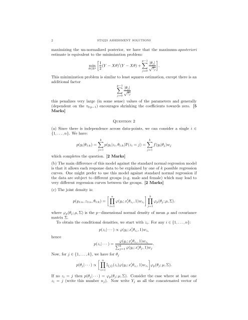
2 <strong>ST5223</strong> <strong>ASSESSMENT</strong> <strong>SOLUTIONS</strong><br />
maximizing the un-normalized posterior, we have that the maximum-aposteriori<br />
estimate is equivalent to the minimization problem:<br />
min<br />
θ∈Rp �<br />
1<br />
2 (Y − Xθ)′ �p−1<br />
�<br />
|θj|<br />
(Y − Xθ) + √ .<br />
τj<br />
j=0<br />
This minimization problem is similar to least squares estimation, except there is an<br />
additional factor<br />
�p−1<br />
j=0<br />
|θj|<br />
√ τj<br />
this penalizes very large (in some sense) values of the parameters and generally<br />
(dependent on the τ0:p−1) encourages shrinking the coefficients towards zero. [5<br />
Marks]<br />
<strong>Question</strong> 2<br />
(a) Since there is independence across data-points, we can consider a single i ∈<br />
{1, . . . , n}. <strong>We</strong> have:<br />
p(yi|θ1:k) =<br />
k�<br />
p(yi|zi, θ1:k)P(zi = j) =<br />
j=1<br />
which completes the question. [2 Marks]<br />
k�<br />
f(yi|θj)wj<br />
(b) The main difference of this model against the standard normal regression model<br />
is that it allows each response data to be explained by one of k possible regression<br />
curves. One might prefer to use this model against standard normal regression if<br />
the data are subject to different groups (e.g. male and female) which may lead to<br />
very different regression curves between the groups. [2 Marks]<br />
(c) The joint density is:<br />
p(y1:n, z1:n, θ1:k) =<br />
i=1<br />
j=1<br />
�<br />
�n<br />
ϕ(yi; x ′ �<br />
�k<br />
iθzi , 1)wzi ϕp(θj; µ, Σ).<br />
where ϕp(θj; µ, Σ) is the p−dimensional normal density of mean µ and covariance<br />
matrix Σ.<br />
To obtain the conditional densities, we start with zi. For any i ∈ {1, . . . , n}:<br />
hence<br />
p(zi| · · · ) ∝ ϕ(yi; x ′ iθzi , 1)wzi<br />
j=1<br />
p(zi| · · · ) = ϕ(yi; x ′ θzi i , 1)wzi<br />
�k j=1 ϕ(yi; x ′ iθj, .<br />
1)wj<br />
Now, for j ∈ {1, . . . , k}, we have for θj<br />
�<br />
�n<br />
p(θj| · · · ) ∝ I {j}(zi)ϕ(yi; x ′ �<br />
iθzi , 1)wzi ϕp(θj; µ, Σ).<br />
i=1<br />
If no zi = j then p(θj| · · · ) = ϕp(θj; µ, Σ). Consider the case where at least one<br />
zi = j (write this number nj). Now write Yj as all the concatenated vector of


