ST5223 ASSESSMENT SHEET 1 SOLUTIONS Question 1 (a) We ...
ST5223 ASSESSMENT SHEET 1 SOLUTIONS Question 1 (a) We ...
ST5223 ASSESSMENT SHEET 1 SOLUTIONS Question 1 (a) We ...
Create successful ePaper yourself
Turn your PDF publications into a flip-book with our unique Google optimized e-Paper software.
<strong>ST5223</strong> <strong>ASSESSMENT</strong> <strong>SHEET</strong> 1 <strong>SOLUTIONS</strong><br />
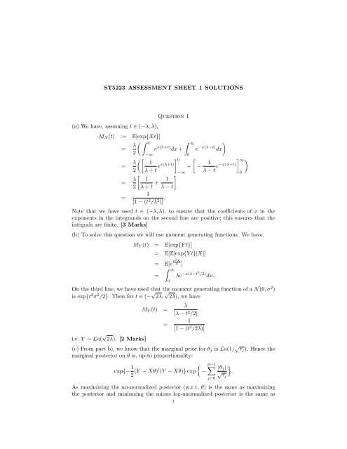
(a) <strong>We</strong> have, assuming t ∈ (−λ, λ),<br />
<strong>Question</strong> 1<br />
MX(t) := E[exp{Xt}]<br />
= λ<br />
� � 0<br />
2<br />
= λ<br />
��<br />
1<br />
2 λ + t ex(λ+t)<br />
�0 = λ<br />
� �<br />
1 1<br />
+<br />
2 λ + t λ − t<br />
=<br />
e<br />
−∞<br />
x(λ+t) dx +<br />
1<br />
[1 − (t 2 /λ 2 )] .<br />
−∞<br />
� ∞<br />
0<br />
e −x(λ−t) �<br />
dx<br />
�<br />
+ − 1<br />
λ − t e−x(λ−t)<br />
�∞� Note that we have used t ∈ (−λ, λ), to ensure that the coefficients of x in the<br />
exponents in the integrands on the second line are positive; this ensures that the<br />
integrals are finite. [3 Marks]<br />
(b) To solve this question we will use moment generating functions. <strong>We</strong> have<br />
MY (t) = E[exp{Y t}]<br />
= E[E[exp{Y t}|X]]<br />
= E[e t2 X<br />
2 ]<br />
=<br />
� ∞<br />
0<br />
λe −x(λ−t2 /2) dx.<br />
On the third line, we have used that the moment generating function of a N (0, σ 2 )<br />
is exp{t 2 σ 2 /2}. Then for t ∈ (− √ 2λ, √ 2λ), we have<br />
i.e. Y ∼ La( √ 2λ). [2 Marks]<br />
MY (t) =<br />
=<br />
λ<br />
[λ − t2 /2]<br />
1<br />
[1 − (t2 /2λ)]<br />
(c) From part b), we know that the marginal prior for θj is La(1/ √ τj). Hence the<br />
marginal posterior on θ is, up-to proportionality:<br />
exp{− 1<br />
2 (Y − Xθ)′ �<br />
(Y − Xθ)} exp<br />
�p−1<br />
−<br />
j=0<br />
|θj|<br />
�<br />
√ .<br />
τj<br />
As maximizing the un-normalized posterior (w.r.t. θ) is the same as maximizing<br />
the posterior and minimzing the minus log-unormalized posterior is the same as<br />
1<br />
0
2 <strong>ST5223</strong> <strong>ASSESSMENT</strong> <strong>SOLUTIONS</strong><br />
maximizing the un-normalized posterior, we have that the maximum-aposteriori<br />
estimate is equivalent to the minimization problem:<br />
min<br />
θ∈Rp �<br />
1<br />
2 (Y − Xθ)′ �p−1<br />
�<br />
|θj|<br />
(Y − Xθ) + √ .<br />
τj<br />
j=0<br />
This minimization problem is similar to least squares estimation, except there is an<br />
additional factor<br />
�p−1<br />
j=0<br />
|θj|<br />
√ τj<br />
this penalizes very large (in some sense) values of the parameters and generally<br />
(dependent on the τ0:p−1) encourages shrinking the coefficients towards zero. [5<br />
Marks]<br />
<strong>Question</strong> 2<br />
(a) Since there is independence across data-points, we can consider a single i ∈<br />
{1, . . . , n}. <strong>We</strong> have:<br />
p(yi|θ1:k) =<br />
k�<br />
p(yi|zi, θ1:k)P(zi = j) =<br />
j=1<br />
which completes the question. [2 Marks]<br />
k�<br />
f(yi|θj)wj<br />
(b) The main difference of this model against the standard normal regression model<br />
is that it allows each response data to be explained by one of k possible regression<br />
curves. One might prefer to use this model against standard normal regression if<br />
the data are subject to different groups (e.g. male and female) which may lead to<br />
very different regression curves between the groups. [2 Marks]<br />
(c) The joint density is:<br />
p(y1:n, z1:n, θ1:k) =<br />
i=1<br />
j=1<br />
�<br />
�n<br />
ϕ(yi; x ′ �<br />
�k<br />
iθzi , 1)wzi ϕp(θj; µ, Σ).<br />
where ϕp(θj; µ, Σ) is the p−dimensional normal density of mean µ and covariance<br />
matrix Σ.<br />
To obtain the conditional densities, we start with zi. For any i ∈ {1, . . . , n}:<br />
hence<br />
p(zi| · · · ) ∝ ϕ(yi; x ′ iθzi , 1)wzi<br />
j=1<br />
p(zi| · · · ) = ϕ(yi; x ′ θzi i , 1)wzi<br />
�k j=1 ϕ(yi; x ′ iθj, .<br />
1)wj<br />
Now, for j ∈ {1, . . . , k}, we have for θj<br />
�<br />
�n<br />
p(θj| · · · ) ∝ I {j}(zi)ϕ(yi; x ′ �<br />
iθzi , 1)wzi ϕp(θj; µ, Σ).<br />
i=1<br />
If no zi = j then p(θj| · · · ) = ϕp(θj; µ, Σ). Consider the case where at least one<br />
zi = j (write this number nj). Now write Yj as all the concatenated vector of
<strong>ST5223</strong> <strong>ASSESSMENT</strong> <strong>SOLUTIONS</strong> 3<br />
response variables with zi = j and write Xj as the associated design matrix. Then<br />
we have<br />
p(θj| · · · ) ∝ ϕnj (Yj; X ′ jθj, Inj×nj )ϕp(θj; µ, Σ).<br />
Recalling from problem sheet 1 that:<br />
(Yj − Xjθj) ′ (Yj − Xjθj) + (θj − µ) ′ Σ −1 (θj − µ) = (θj − µ ∗ j ) ′ Σ ∗−1<br />
j (θj − µ ∗ j ) + b ∗<br />
where<br />
µ ∗ j = Σ ∗ j (Σ ∗−1<br />
j µj + X ′ jYj)<br />
Σ ∗ j = (Σ −1<br />
j + X′ jXj)<br />
and b∗ is a constant that doesn’t depend upon θ. Hence we have that<br />
θj| · · · ∼ Np(µ ∗ j , Σ ∗ j ).<br />
Thus a Gibbs sampler, for a single iteration (to move from z1:n, θ1:k to z ′ 1:n, θ ′ 1:k ) is:<br />
• Sample p(z ′ 1|z2:n, θ1:k, y1:n), p(z ′ 2|z ′ 1, z3:n, θ1:k, y1:n), . . . , p(z ′ n|z ′ 1:n−1, θ1:k, y1:n).<br />
• Sample p(θ ′ 1|z ′ 1:n, θ2:k, y1:n), p(θ ′ 2|z ′ 1:n, θ ′ 1, θ2:k, y1:n), . . . , p(θ ′ k |z′ 1:n, θ ′ 1:k−1 , y1:n).<br />
[6 Marks]


