SAXS data reduction for the absolute intensity scale

SAXS data reduction for the absolute intensity scale
U-Ser Jeng, National Synchrotron Radiation Research Center, Taiwan
Sep. 6. 2004
The SAXS data normalized for scattering cross-section per unit sample volume
is termed as "absolute intensity I(Q)". The absolute intensity scale for the SAXS data
is easy in comparing the scattering powers between different samples, measured at
different instruments or different sample scattering volumes, and is also very useful in
model fitting. SAXS data in the absolute scattering scale requires many details during
the measurement. In practical measurements, the photons collected by the detector per
second, namely, the scattering intensity Is(Q) of a sample is proportional to the
incident beam intensity Io, the scattering differential cross-section per unit volume of
the sample I(Q) = (dΣ(Q)/dΩ)/V (defined as the absolute intensity, with the often used
unit cm -1 ), the sample exposure area A (usually the beam size), sample thickness t,
sample transmission T, the detector view angle for accepting photons ∆Ω (detector slit
opening), and the detector efficiency e, and can be expressed as
I o
S ( Q)
= I I(
Q)
A t T ∆Ω e.
With Is(Q) measured, we can use (1) to factor out sample geometrical factors (t,
T), and instrument parameters (Io, A, ∆Ω, and e), and extract the absolute intensity
I(Q). Such a process is called SAXS data reduction.
During the data reduction, we usually can measure easily the sample thickness,
sample transmission. As to other instrument-related factors, like incident flux, beam
size, view angle, and detector efficiency, we often use a standard sample of known
I(Q) to deduce the common instrument factor f (= IoA∆Ωe), using the Is(Q) measured
under a specific instrumental setting (for instance the sample-to-detector distance,
beam size, wavelength, and detector efficiency, the detecting view angle for each
pixel).
For data reduction, the information of sample transmission is needed in Eq. (1).
In optimizing the sample thickness in a SAXS measurement, we take the thickness
derivative to (1), d(Is)/dt=0, and obtain an optimize sample transmission T = e -1 for
the best scattering intensity. From the optimized T, we can deduce the optimum
sample thickness t = 1/µ, where µ is the absorption coefficient of the sample and can
(1)

e found conveniently from the website:
www-cxro.lbl.gov/optical_constants/atten2.html. Stable materials with high scattering
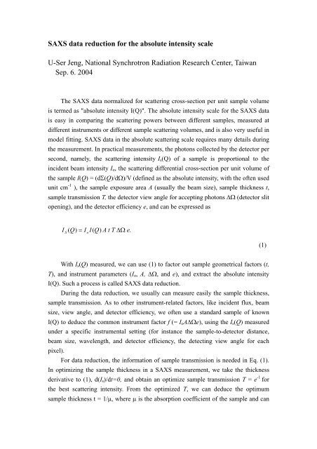
intensity, for instance polyethylene (PE) of a known peak value I(Q) = 36.6 cm -1 at Q
= 0.0223 Å -1 , can be used as secondary standard samples (see Figure 18). With a
standard sample of known absolute I(Q) measured at a SAXS instrument, we can
measure all other related quantities in (1), and determine the f factor for the SAXS
instrument configuration. Using this f factor in (1) for other samples, we can put the
scattering intensity of the samples in the absolute scattering intensity scale I(Q).
In practical data reduction, we still need to consider the subtraction of
background scattering, electronic dark current, and correction for the detector pixel
efficiency. For a normalization for the time-dependent incoming flux for each
measurement, we modify (1) to the following:
dΣ(
Q)
I(
Q)
=
dΩ
1
T
s d s emp
d emp
fTmt
Temp
⎥ ⎥ ⎛ ⎞⎡
⎤
= ⎜
⎟
⎟⎢
⎝ ⎠⎢⎣
⎦
(2)
m
( I ( Q)
−cI
( Q)
) / i − ( I ( Q)
−c"
I ( Q)
) / i / I ( Q)
In (2), is, and iemp are the monitor counts of the incoming beam intensities for the
sample and background SAXS measurements. Whereas c and c'' are the time ratios of
the sample and background scattering measurements to the dark current measurement,
respectively. Tm is the sample transmission measured and Tem is the transmission
measured without sample (air or pure solvent used), whereas Isen(Q) is the detector
efficiency for the corresponding detector pixel. The working procedure for the data
reduction is detailed in the appendix A5.
sen

PE Absolute Intensity dΣ(Q)/dΩ (cm -1 )
10
1
0.1
0.05 0.10
Q (Å -1 )
Figure 18. The commonly used high density polyethylene sample for the absolute
intensity calibration, with a well calibrated intensity at I (Q = 0.0223 Å -1 ) = 36.5 cm -1 .