3.4 The Point-Slope Form of a Line

3.4 The Point-Slope Form of a Line 

Section 3.4 The Point-Slope Form of a Line 293 

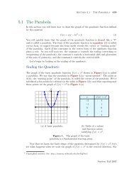
In the last section, we developed the slope-intercept form of a line (y = mx + b). The 

slope-intercept form of a line is applicable when you’re given the slope and y-intercept 

of the line. However, there will be times when the y-intercept is unknown. 

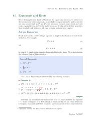
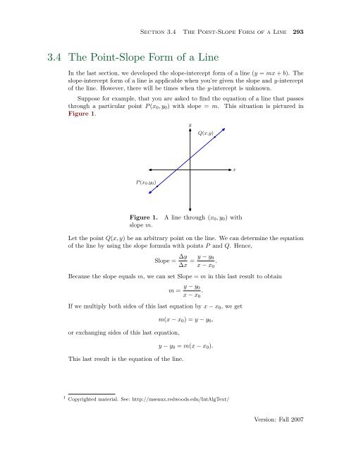
Suppose for example, that you are asked to find the equation of a line that passes 

through a particular point P (x0, y0) with slope = m. This situation is pictured in 

Figure 1. 

P (x0,y0) 

y 

Q(x,y) 

Figure 1. A line through (x0, y0) with 

slope m. 

Let the point Q(x, y) be an arbitrary point on the line. We can determine the equation 

of the line by using the slope formula with points P and Q. Hence, 

Slope = ∆y 

∆x 

y − y0 

= . 

x − x0 

Because the slope equals m, we can set Slope = m in this last result to obtain 

m = 

y − y0 

. 

x − x0 

If we multiply both sides of this last equation by x − x0, we get 

or exchanging sides of this last equation, 

This last result is the equation of the line. 

m(x − x0) = y − y0, 

y − y0 = m(x − x0). 

1 

Copyrighted material. See: http://msenux.redwoods.edu/IntAlgText/ 

x 

Version: Fall 2007

294 Chapter 3 Linear Functions 

The Point-Slope Form of a Line. If line L passes through the point (x0, y0) 

and has slope m, then the equation of the line is 

Version: Fall 2007 

y − y0 = m(x − x0). (1) 

This form of the equation of a line is called the point-slope form. 

To use the point-slope form of a line, follow these steps. 

Procedure for Using the Point-Slope Form of a Line. When given the slope 

of a line and a point on the line, use the point-slope form as follows: 

1. Substitute the given slope for m in the formula y − y0 = m(x − x0). 

2. Substitute the coordinates of the given point for x0 and y0 in the formula 

y − y0 = m(x − x0). 

For example, if the line has slope −2 and passes through the point (3, 4), then 

substitute m = −2, x0 = 3, and y0 = 4 in the formula y − y0 = m(x − x0) to 

obtain 

y − 4 = −2(x − 3). 

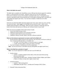
◮ Example 2. Draw the line that passes through the point P (−3, −2) and has slope 

m = 1/2. Use the point-slope form to determine the equation of the line. 

First, plot the point P (−3, −2), as shown in Figure 2(a). Starting from the point 

P (−3, −2), move 2 units to the right and 1 unit up to the point Q(−1, −1). The line 

through the points P and Q in Figure 2(a) now has slope m = 1/2. 

P (−3,−2) 

Q(−1,−1) 

∆x=2 

y 

∆y=1 

(a) The line through P (−3, −2) 

with slope m = 1/2. 

x 

Figure 2. 

y 

R(0,−0.5) 

(b) Checking the y-intercept. 

x


To determine the equation of the line in Figure 2(a), we will use the point-slope form 

of the line 

y − y0 = m(x − x0). (3) 

The slope of the line is m = 1/2 and the given point is P (−3, −2), so (x0, y0) = 

(−3, −2). In equation (3), set m = 1/2, x0 = −3, and y0 = −2, obtaining 

or equivalently, 

y − (−2) = 1 

(x − (−3)), 

2 

This is the equation of the line in Figure 2(a). 

y + 2 = 1 

(x + 3). (4) 

2 

As a check, we’ve estimated the y-intercept of the line in Figure 2(b) as R(0, −0.5). 

Let’s place equation (4) in slope-intercept form to determine the exact value of the 

y-intercept. First, distribute 1/2 to get 

y + 2 = 1 3 

x + 

2 2 . 

Subtract 2 from both sides of this last equation. 

y = 1 3 

x + − 2 

2 2 

Make equivalent fractions with a common denominator and simplify. 

y = 1 3 4 

x + − 

2 2 2 

y = 1 1 

x − 

2 2 

Comparing equation (5) with y = mx+b gives us b = −1/2. This is the exact y-value 

of the y-intercept. Note that this result compares exactly with the y-value of point R 

in Figure 2(b). This is a bit lucky. Don’t expect to get an exact comparison every 

time. However, if the comparison is not close, look for an error in your work, either in 

your computations or in your graph. 

Let’s look at another example. 

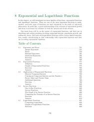
◮ Example 6. Find the equation of the line passing through the points P (−3, 2) 

and Q(2, −1). Place your final answer in standard form. 

Again, to help keep our focus, we draw the line passing through the points P (−3, 2) 

and Q(2, −1) in Figure 3. 

(5) 

Version: Fall 2007



P (−3,2) 

y 

Q(2,−1) 

Figure 3. The line through points 

P (−3, 2) and Q(2, −1). 

Use the slope formula to determine the slope of the line through the points P (−3, 2) 

and Q(2, −1). 

We’ll use the point-slope form of the line 

m = ∆y −1 − 2 

= = −3 

∆x 2 − (−3) 5 

x 

y − y0 = m(x − x0). (7) 

Let’s use point P (−3, 2) as the given point (x0, y0). That is, (x0, y0) = (−3, 2). Substitute 

m = −3/5, x0 = −3, and y0 = 2 in equation (7), obtaining 

y − 2 = − 3 

(x − (−3)). (8) 

5 

This is the equation of the line passing through the points P and Q. 

Alternatively, we could also use the point Q(2, −1) as the given point (x0, y0). That 

is, (x0, y0) = (2, −1). Substitute m = −3/5, x0 = 2, and y0 = −1 in the point-slope 

form (7), obtaining 

y − (−1) = − 3 

(x − 2). (9) 

5 

This too, is the equation of the line passing through the points P and Q. 

How can the equations (8) and (9) both be the equation of the line through P 

and Q, yet look so distinctly different? Let’s place each equation in standard form 

Ax + By = C and compare the results. 

If we start with equation (8) and distribute the slope, 

y − 2 = − 3 

(x − (−3)) 

5 

y − 2 = − 3 9 

x − 

5 5 . 

Multiply both sides by the common denominator 5 to clear the fractions.


� 

5(y − 2) = 5 − 3 

� 

9 

x − 

5 5 

5y − 10 = −3x − 9 

Add 3x to both sides of the equation, then add 10 to both sides of the equation to 

obtain 

3x + 5y = 1. (10) 

Place equation (9) in standard form in a similar manner. First, start with equation (9) 

and distribute the slope, 

y − (−1) = − 3 

(x − 2) 

5 

y + 1 = − 3 6 

x + 

5 5 . 

Next, multiply both sides of this last result by 5 to clear the fractions from the equation. 

� 

5 (y + 1) = 5 − 3 

� 

6 

x + 

5 5 

5y + 5 = −3x + 6 

Finally, add 3x to both sides of the equation, then subtract 5 from both sides of the 

equation to obtain 

3x + 5y = 1. (11) 

Note that equation (11) is identical to equation (10). Thus, it doesn’t matter which 

point you use in the point-slope form. Both lead to the same result. 

Parallel Lines 

Recall that slope controls the “steepness” of a line. Consequently, if two lines are 

parallel, they must have the same “steepness” or slope. Let’s look at an example of 

parallel lines. 

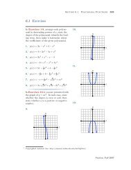
◮ Example 12. Find the equation of the line that passes through the point P (−2, 2) 

that is parallel to the line passing through the points Q(−3, −1) and R(2, 1). 

First, to help us stay focused, we draw the line through the points Q(−3, −1) and 

R(2, 1), then plot the point P (−2, 2), as shown in Figure 4(a). 

We can use the slope formula to calculate the slope of the line passing through the 

points Q(−3, −1) and R(2, 1). 

m = ∆y 1 − (−1) 2 

= = 

∆x 2 − (−3) 5 

Version: Fall 2007


P (−2,2) 


Q(−3,−1) 

y 

R(2,1) 

(a) The line through 

Q(−3, −1) and R(2, 1). 

x 

Figure 4. 

P (−2,2) 

Q(−3,−1) 

y 

∆x=5 

T (3,4) 

R(2,1) 

∆y=2 

(b) The line through P (−2, 2) 

that is parallel to the 

line through Q and R. 

We now draw a line through the point P (−2, 2) that is parallel to the line through 

the points Q and R. Parallel lines must have the same slope, so we start at the point 

P (−2, 2), “run” 5 units to the right, then “rise” 2 units up to the point T (3, 4), as 

shown in Figure 4(b). 

We seek the equation of the line through the points P and T . We’ll use the pointslope 

form of the line 

y − y0 = m(x − x0). (13) 

We’ll use the point P (−2, 2) as the given point (x0, y0). That is, (x0, y0) = (−2, 2). 

The line through P has slope 2/5. Substitute m = 2/5, x0 = −2, and y0 = 2 in 

equation (13) to obtain 

y − 2 = 2 

(x − (−2)). (14) 

5 

Let’s place the equation (14) in standard form. Distribute the slope, then clear 

fractions by multiplying both sides of the resulting equation by 5. 

y − 2 = 2 4 

x + 

5� 5 � 

2 4 

5(y − 2) = 5 x + 

5 5 

5y − 10 = 2x + 4 

Finally, subtract 5y from both sides of the last equation, then subtract 4 from both 

sides of the equation, obtaining 


−14 = 2x − 5y, 

x


2x − 5y = −14. 

This is the standard form of the equation of the line passing through the point P and 

parallel to the line passing through the points Q and R. 

Perpendicular Lines 

Suppose that two lines L1 and L2 have slopes m1 and m2, respectively. Recall (see the 

section on Slope) that if L1 and L2 are perpendicular, then the product of their slopes 

is m1m2 = −1. Alternatively, the slope of the first line is the negative reciprocal of 

the second line, and vice-versa; i.e., m1 = −1/m2 and m2 = −1/m1. Let’s look at an 

example of perpendicular lines. 

◮ Example 15. Find the equation of the line passing through the point P (−4, −4) 

that is perpendicular to the line 4x + 3y = 12. 

It will help our focus if we draw the given line 4x + 3y = 12. The easiest way to 

plot a line in standard form Ax + By = C is to find the x- and y-intercepts. 

4x + 3y = 12 4x + 3y = 12 

4x + 3(0) = 12 4(0) + 3y = 12 

4x = 12 3y = 12 

x = 3 y = 4 

Plot the x- and y-intercepts R(3, 0) and S(0, 4) as shown in Figure 5(a). The line 

through points R and S is the graph of the equation 4x + 3y = 12. 

y 

S(0,4) 

R(3,0) 

x 

(a) Plot the x and 

y-intercepts of 4x + 3y = 12. 

P (−4,−4) 

Figure 5. 

Q(0,−1) 

∆x=4 

y 

∆y=3 

(b) A line through P (−4, −4) that 

is perpendicular to 4x + 3y = 12. 

x 

m=−4/3 

Next, determine the slope of the line 4x + 3y = 12 by placing this equation in 

slope-intercept form (i.e., solve the equation 4x + 3y = 12 for y). 2 

Version: Fall 2007



4x + 3y = 12 

3y = −4x + 12 

y = − 4 

x + 4 

3 

If two lines are perpendicular, then their slopes are negative reciprocals of one 

another. Therefore, the slope of the line that is perpendicular to the line 4x + 3y = 12 

(which has slope −4/3) is m = 3/4. Our second line must pass through the point 

P (−4, −4). To draw this second line, first plot the point P (−4, −4), then move 4 units 

to the right and 3 units upward to the point Q(0, −1), as shown in Figure 5(b). The 

line through the points P and Q is perpendicular to the line 4x + 3y = 12. 3 

To determine the equation of the line through the points P and Q, we will use the 

point-slope form of the line, namely 

y − y0 = m(x − x0). (16) 

The slope of the line through points P and Q is m = 3/4. If we use the point P (−4, −4), 

then (x0, y0) = (−4, −4). Set m = 3/4, x0 = −4, and y0 = −4 in equation (16), 

obtaining 


y − (−4) = 3 

(x − (−4)), 

4 

y + 4 = 3 

(x + 4). (17) 

4 

Alternatively, we could use the slope-intercept form of the line. We know that the 

line through points P and Q in Figure 5(b) crosses the y-axis at Q(0, −1). So, with 

slope m = 3/4 and y-coordinate of the y-intercept b = −1, the slope-intercept form 

y = mx + b becomes 

y = 3 

x − 1. 

4 

On the other hand, if we solve equation (17) for y, 

y + 4 = 3 

(x + 4) 

4 

y + 4 = 3 

x + 3 

4 

y = 3 

x − 1. 

4 

Note that this is identical to the result found using the slope-intercept form above. 

2 If you also remember that the slope of Ax + By = C is m = −A/B, then the slope of 4x + 3y = 12 is 

m = −A/B = −4/3. 

3 It’s a good exercise to measure the angle between the two lines with a protractor. If the angle measures 

90 degrees, then you know the lines are truly perpendicular. 

(18)


It is comforting to note that the two forms (point-slope and slope-intercept) give 

the same result, but how do we determine the most efficient form to use for a particular 

problem? Here’s a good hint. 

Determining the Form of the Line to Use. Here is some sound advice when 

you are trying to determine whether to use the slope-intercept form or the pointslope 

form of a line. 

• If you are given the slope and the y-intercept, use the slope-intercept form 

y = mx + b. 

• If you are given a point (other than the y-intercept) and the slope, use the 

point-slope form y − y0 = m(x − x0). 

Applications of Linear Functions 

In this section we will look at some applications of linear functions. We begin by 

developing a function relating Fahrenheit and Celsius temperature. 

◮ Example 19. Water freezes at 32 ◦ F and 0 ◦ C. Water boils at 212 ◦ F and 100 ◦ C. 

F and C are abbreviations for Fahrenheit and Celsius temperature scales, respectively. 

Assuming a linear relationship, develop a model relating Fahrenheit and Celsius temperature. 

First, to help keep our focus, we set up a coordinate system on a sheet of graph 

paper. In Figure 6, we’ve decided to make the Celsius temperature the dependent 

variable and have assigned the Celsius temperature to the vertical axis. Similarly, 

we’ve declared the Fahrenheit temperature the independent variable and assigned it to 

the horizontal axis. 4 

Interpret the given data: 

• Water freezes at 32 ◦ F and 0 ◦ C. This gives us the point (F, C) = (32, 0), which we 

plot in Figure 6. 

• Water boils at 212 ◦ F and 100 ◦ C. This gives us the point (F, C) = (212, 100), which 

we plot in Figure 6. 

Now we are on familiar ground. We want to find the equation of the line through 

these two points, which is the same type of problem we tackled in Example 6. First, 

use the points (32, 0) and (212, 100) to determine the slope of the line. 

m = ∆C 

∆F 

100 − 0 100 5 

= = = 

212 − 32 180 9 . 

We will now use the point-slope form of the line, y − y0 = m(x − x0) with m = 5/9 and 

(x0, y0) = (32, 0). Substitute m = 5/9, x0 = 32, and y0 = 0 in y − y0 = m(x − x0) to 

obtain 

4 We could easily reverse these assignments, placing the Fahrenheit temperature on the vertical axis and 

the Celsius temperature on the horizontal axis. 

Version: Fall 2007



120 

C 

(32, 0) 

(212, 100) 

F 

250 

Figure 6. Plotting Celsius temperature versus Fahrenheit 

temperature. 

y − 0 = 5 

(x − 32). (20) 

9 

However, our dependent axis is labeled C, not y, and our independent axis is labeled 

F , not x. So, we must replace y and x in equation (20) with C and F , respectively, 

obtaining 

C = 5 

(F − 32). (21) 

9 

This result in equation (21) expresses the Celsius temperature as a function of the 

Fahrenheit temperature. Alternatively, we could also use function notation and write 

C(F ) = 5 

(F − 32). 

9 

Suppose that we know that the Fahrenheit temperature outside is 80 ◦ F and we 

wish to express this using the Celsius scale. To do so, we simply evaluate C(80), as in 

C(80) = 5 

(80 − 32) ≈ 26.6. 

9 

Hence, the Celsius temperature is approximately 26.6 ◦ C. 

On the other hand, suppose that we know the Celsius temperature on a metal roof 

is 80 ◦ C and we wish to find the Fahrenheit temperature. To do so, we need to solve 

for F , or equivalently, 

Multiply both sides by 9 to obtain 

C(F ) = 80 

5 

(F − 32) = 80. 

9 

5(F − 32) = 720,

then divide both sides of the result by 5 to obtain 


F − 32 = 144. 

Adding 32 to both sides of this last result produces the Fahrenheit temperature F = 

176 ◦ F. Wow, that’s hot! 

Version: Fall 2007

3.4 The Point-Slope Form of a Line

Create successful ePaper yourself

Delete template?

Save as template?