Temprature-variations-and-control-of-calciner.pdf
Temprature-variations-and-control-of-calciner.pdf
Temprature-variations-and-control-of-calciner.pdf

You also want an ePaper? Increase the reach of your titles
YUMPU automatically turns print PDFs into web optimized ePapers that Google loves.
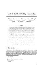
Temperature <strong>variations</strong> <strong>and</strong> <strong>control</strong> <strong>of</strong> a Calciner<br />
1 Background<br />
Elkem<br />
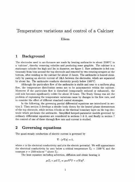
The electrodes used in arc-furnaces are made by heating anthracite to about 2500°C in<br />
a '<strong>calciner</strong>', thereby removing volatiles <strong>and</strong> producing some graphite. The <strong>calciner</strong> is a<br />
stationary cylinder 8m high <strong>and</strong> 2m in diameter, see figure 1. Raw anthracite is fed continuously<br />
from bins around the top electrode <strong>and</strong> removed by two rotating scrapers at the<br />
bottom, after residing in the <strong>calciner</strong> for about 15 hours. The anthracite is heated ohmically<br />
by passing an electric current <strong>of</strong> 14kA between the electrodes, which are separated<br />
by about 3m. The anthracite conducts electricity poorly below 1500°C.<br />
Although the particulate flow <strong>of</strong> the anthracite is stable <strong>and</strong> near to a uniform plug<br />
flow, the temperature distribution seems not to be axisymmetric within the <strong>calciner</strong>.<br />
Moreover if the particulate flow is disturbed (temporarily reduced or enhanced), the<br />
cold side becomes significantly colder for about 10 hours. The Study Group was set the<br />
problem <strong>of</strong> explaining the temperature <strong>variations</strong> cause by changes in the flow rate, <strong>and</strong><br />
to consider the effect <strong>of</strong> different st<strong>and</strong>ard <strong>control</strong> strategies.<br />
In the following, the governing partial differential equations are introduced in section<br />
2. Then section 3 develops a slender body theory for the heated plume downstream<br />
<strong>of</strong> the top electrode, while section 4 looks at the thermal boundary layer on the top electrode<br />
which pre-heats the anthracite. Simplified lumped-parameter models governed by<br />
ordinary differential equations are considered in sections 5 & 6, <strong>and</strong> finally in section 7<br />
the <strong>control</strong> <strong>of</strong> one <strong>of</strong> these through flow rate <strong>and</strong> current is studied.<br />
2 Governing equations<br />
The quasi-steady conduction <strong>of</strong> electric current is governed by<br />
where a is the electrical conductivity <strong>and</strong> fjJ is the electric potential. We will approximate<br />
the electrical conductivity by zero below a critical temperature Tc = 1500 OK <strong>and</strong> the<br />
constant a = 2500 mho m-I above Tc.<br />
The heat equation including advection, diffusion <strong>and</strong> ohmic heating is<br />
1
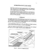
Figure 1 Elkem Ca1ciner<br />
~------- Gas stock<br />
Feedirq bins<br />
Electrode holder<br />
Secoodory bus bars<br />
FUrnace cover<br />
Top electrode<br />
Furnace shell with lining<br />
Bottom electrode<br />
To the bag filter<br />
Discharge mechanism<br />
Dischorqirq chutes with the<br />
weighing container<br />
Conveyor<br />
2<br />
Figure 2 Discharge mechanism
Typical values for the anthracite in the <strong>calciner</strong> are :- density p = 900 kg m -3, specific<br />
heat C = 1700 J kg- 1 oK-I, temperature T = 1500 "K, time t = 6x 10 4 s, advection velocity<br />
U = 1.4 X 10- 4 m s-1, (axial) length L = 5 m, heat conductivity K, = 10- 5 m2 s-1, electrical<br />
conductivity a = 2500 mho m-I, <strong>and</strong> electrical potential
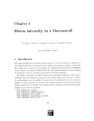
4 Thermal boundary layer on top electrode<br />
Now the electrodes are long <strong>and</strong> are themselves heated ohmically. Along the length <strong>of</strong> the<br />
electrode, heat will diffuse radially out forming a thermal boundary layer in the anthracite<br />
moving along the electrode. It is essential that the anthracite is pre-heated (in sufficient<br />
quantity) to the critical temperature Tc before the end <strong>of</strong> the electrode in order that<br />
thermal plume can conduct electricity.<br />
Let the electrode carry current I, be <strong>of</strong>radius a <strong>and</strong> have a length f. Let the thermal<br />
boundary layer have a thickness t5 at the end <strong>of</strong> the electrode: 6 = (K,fIU)I/2. The time<br />
for anthracite to move along the electrode is flU, so that the total ohmic heating in the<br />
electrode during that time is (I I a 2 )2I oe x a 2 f x flU (dropping factors like 7r), where aE is<br />
the electrical conductivity <strong>of</strong> the electrode. Increasing the temperature <strong>of</strong> the anthracite<br />
to Tc from effectively 0 within the boundary layer requires heat pcTc x Ma. Equating<br />
these two, we find that electrode must be at least as long as<br />
£ = eCT~~Ea3ra:<br />
We use the following values <strong>of</strong> the relevant parameters: density p = 850kgm- 3 ,<br />
specific heat c = 1700 J kg-l oK-I, critical temperature Tc = 1500 OK, conductivity <strong>of</strong><br />
the electrode aE = 10 5 mho m-I, radius <strong>of</strong> electrode a = 0.25 m, total current 1= 14 kA,<br />
advection velocity U = 1.4 x 10- 4 m s"! <strong>and</strong> heat conductivity K, = 1O- 5 m 2 s-1. These<br />
produce the estimate for the length <strong>of</strong> the electrode necessary in order to reach the critical<br />
temperature as f = 0.5 m, which agrees with the Elkem design. At this length, the thermal<br />
boundary layer has a thickness <strong>of</strong> 0.17 m, which is similar to the radius <strong>of</strong> the electrode<br />
in the Elkem design, <strong>and</strong> hence allows an easy transition to the thermal plume.<br />
We note that the required length <strong>of</strong> the electrode f is proportional to the velocity<br />
<strong>of</strong> the anthracite. Hence if the feed is increased too much, there will be insufficient<br />
pre-heating <strong>of</strong> the anthracite to the critical conduction temperature Tc in the thermal<br />
boundary layer.<br />
5 Lumped models<br />
In order to underst<strong>and</strong> the temporal development, <strong>and</strong> possible instability, <strong>of</strong> non-axisymmetric<br />
differences between one side <strong>of</strong> the <strong>calciner</strong> <strong>and</strong> the other, the Study Group<br />
investigated a simple lumped-parameter model. The full temperature field was replaced<br />
by four temperatures: Tl <strong>and</strong> T2 the temperatures in the thermal plume on the left <strong>and</strong><br />
right sides respectively, <strong>and</strong> T3 <strong>and</strong> T4 the temperatures in the thermal boundary layers<br />
again on the left <strong>and</strong> right sides respectively. These temperatures were taken as being<br />
typical <strong>of</strong> their respective region <strong>and</strong> to be only a function <strong>of</strong> time. The temperature <strong>of</strong><br />
the electrode was taken to be T.<br />
The heat balance for the left plume region <strong>of</strong> length L <strong>and</strong> cross-sectional area A is<br />
pcALT1 + pcUA(T1 - T3) = k1(T2 - Td + k2(T3 - Td + k3(T - Td + nI,<br />
with coefficients k; for the heat transfer between different regions, which could be estimated<br />
from the studies above, <strong>and</strong> with ohmic heating n1. The equation for the right<br />
4
plume regions is similar with T2 replacing T1 <strong>and</strong> T4 replacing T3. The heat balance for<br />
the left thermal boundary layer is<br />
<strong>and</strong> a similar equation for the right thermal boundary layer with T2 replacing T1 <strong>and</strong> T4<br />
replacing T 3 .<br />
There was much discussion about the form to be adopted for the ohmic heating.<br />
In the model eventually adopted, most <strong>of</strong> the voltage drop V was taken to occur in the<br />
thermal plume, <strong>and</strong> so<br />
A 2<br />
01 = L 0"(T1)V ,<br />
<strong>and</strong> a similar expression in the right thermal plume with T2 replacing T 1 . The alternative<br />
model which was eventually rejected had most <strong>of</strong> the heating occurring near to the<br />
electrode<br />
01 = 'Y(T1, T)V 2 ,<br />
with the function '1'still to be determined somehow.<br />
More sophisticated models with the cross-sectional area A varying were not pursued.<br />
6 Reduced model<br />
In order to underst<strong>and</strong> the possibility <strong>of</strong> non-axisymmetric states, the above lumpedparameter<br />
model was further simplified by deleting the thermal boundary layers, leaving<br />
the two-variable model<br />
1'1 = -UTI + >'(T2 - T1) + 'Y0"(T1)<br />
1'2 = -UT2 + >'(T1 - T2) + 'Y0"(T2)<br />
Recall that O"(T) = 0 for T < Te <strong>and</strong> O"(T) = 1 for T > Tr: It is important to realise now<br />
that 0" rises very sharply from 0 to 1 in a neighbourhood <strong>of</strong> Tc, <strong>and</strong> so we may consider<br />
it to take on arbitrary values between 0 <strong>and</strong> 1 for T = Te.<br />
If U > '1'ITe, the only solution is the symmetric solution T1 = T2 = 0, i.e. too cold<br />
for any ohmic heating.<br />
If U < '1'ITe, there are three symmetric solutions<br />
T1 = T2 = 0, Te <strong>and</strong> 'YIU,<br />
corresponding to no heating (0" = 0), partial heating (0" = UTel'Y) <strong>and</strong> full heating<br />
(0" = 1), respectively.<br />
If '1'(>.+ U)ITe(2)' + U) > U > 'Y>'ITc(2)' + U), there are also two asymmetric<br />
solutions with full heating in one side O"(Td = 1 <strong>and</strong> no heating in the other 0"(T2) = 0<br />
'1'(>.+ U)<br />
T, = U (2)' + U) ,<br />
<strong>and</strong> a similar solution with T, <strong>and</strong> T2 interchanged.<br />
5
If ,ITe > U > ,)..ITe(2)"+U), there are two asymmetric solutions with full heating<br />
on one side a(Td = 1 <strong>and</strong> partial heating on the other T2 = Te<br />
T _ ,+)"Te<br />
1- )..+U '<br />
T - T. . h _ U(2)" + U)Te - )..,<br />
2 - e WIt ae - ()..+ Uh '<br />
<strong>and</strong> a similar solution with T, <strong>and</strong> T2 interchanged.<br />
Finally if U < ,(),,+U)ITc(2)"+U), there are two asymmetric solutions with partial<br />
heating on one side T, = Te <strong>and</strong> no heating on the other a(T2) = °<br />
. U(2)" + U)Te<br />
'T, = Te with ae = ()..+ Uh '<br />
<strong>and</strong> a similar solution with Tl <strong>and</strong> T2 interchanged.<br />
A simple phase-plane analysis find that the solutions with some partial heating are<br />
all unstable (saddle points or unstable nodes). At high flow rates U > ,ITe the only<br />
stable solution is the cold symmetric state T, = T2 = 0, i.e. the anthracite fails to reach<br />
the critical temperature before it passes out <strong>of</strong> the <strong>calciner</strong> <strong>and</strong> so in this simplified model<br />
there is no heating anywhere. At lower flow rates U < ,ITe, in addition to this cold stable<br />
symmetric state there is the symmetric state Tl = T2 = ,IU, in which ohmic heating<br />
can exceed the critical temperature before the material exits the <strong>calciner</strong>. In the range<br />
,()..+ U)ITe(2)" + U) > U > ,)..ITe(2)" + U) there are also two stable asymmetric states,<br />
one side with ohmic heating <strong>and</strong> one without. In these asymmetric states, the ohmic<br />
heating on the one side is sufficient for the anthracite to reach the critical temperature<br />
on that side, but via heat transfer between the two sides is insufficient for the other side.<br />
Clearly one way to eliminate the asymmetric state would be to decrease the flow rate<br />
until U < ,)..ITe(2)" + U).<br />
Future work should incorporate the electrode into the two-variable theory, <strong>and</strong> to<br />
return to the four-variable theory <strong>of</strong> section 5 which could be solved numerically.<br />
7 Control<br />
The Study Group considered the <strong>control</strong> <strong>of</strong> the two-variable model <strong>of</strong> section 6 through<br />
monitoring the total current I = A( a(T1) + a(T2)) VI L <strong>and</strong> in response adjusting the flow<br />
U <strong>of</strong> the anthracite. It is to be expected that some <strong>control</strong> mechanisms U = f (1) might<br />
be unstable: the time-delay resulting from the non-zero residence time (not in the model<br />
<strong>of</strong> section 6) may require responding to the time-integral <strong>of</strong> the current rather than the<br />
instantaneous value in order to avoid <strong>control</strong> instabilities.<br />
The simplest <strong>control</strong> strategy is 'bang-bang', in which either the flow runs at its<br />
normal constant value, U = U say, if both sides <strong>of</strong> the thermal plume are being ohmically<br />
heated, I > 2Aa(Te+) VI L, or the flow is shut down totally, U = 0, if both sides are not<br />
above the critical temperature for ohmic heating.<br />
Under bang-bang <strong>control</strong>, if the initial state has ohmic heating on both sides, T, > Te<br />
<strong>and</strong> T2 > Te, then the system will evolve to the stable symmetric state with ohmic<br />
heating, T, = T2 = ,IU, so long as the flow is sufficiently slow for this state to exist,<br />
U < ,IT e. This follows immediate from the governing equations in this regime<br />
TI + T2 = -U(Tl + T2) + 2" <strong>and</strong> i,- T2 = -(U + 2)")(T1 - T2).<br />
6
If on the other h<strong>and</strong> the initial state has no ohmic heating on both sides, the system<br />
would evolve under bang-bang <strong>control</strong> to a symmetric state at the average <strong>of</strong> the initial<br />
temperatures, <strong>and</strong> no ohmic heating. Again this immediately follows from the governing<br />
equations in this regime<br />
The initial condition <strong>of</strong> one side ohmically heated <strong>and</strong> the other not, as would occur<br />
in the stable asymmetric states, is more complicated. If one side is significantly above<br />
the critical temperature <strong>and</strong> the other side is only just below, then the cold side will<br />
warm up to the critical temperature <strong>and</strong> the system will then evolve into the stable<br />
symmetric state with both sides heated ohmically. If one side is only just above the<br />
critical temperature <strong>and</strong> the other side is significantly below, then the hot side may cool<br />
down to the critical temperature, with the system then evolving into a symmetric state<br />
with no ohmic heating, or if the rate <strong>of</strong> heating is high enough the cold side may warm up<br />
to the critical temperature. To distinguish between these different cases, we consider the<br />
governing equations for the left side being heated T, > Te <strong>and</strong> the right side not T2 < Te<br />
with solution<br />
dD 2),<br />
-=--D+1<br />
dS ,<br />
D = .i. + (D _~) -2(8-80»';-y<br />
2), 0 2), e ,<br />
where Do <strong>and</strong> So are the initial values.<br />
We now need to write down the boundaries <strong>of</strong> this regime <strong>of</strong> one sided heated <strong>and</strong><br />
the other not in terms <strong>of</strong> the new variables D <strong>and</strong> S. The constraint that Tl > Te <strong>and</strong><br />
o < T2 < Te gives D > 0 <strong>and</strong> S > Te at least. The right side will warm up to the critical<br />
temperature while the left side is still hot if according to the above solution T2 = Te<br />
while T, > Te, i.e. D = S - 2Te in S > 2Te. The left side will cool down to the critical<br />
temperature while the right remains cold if T, = Te while T2 < Tn, i.e. D = 2Te - S in<br />
Te < S < 2Te.<br />
From the solution D(S) it is clear that if the rate <strong>of</strong> heating is sufficiently large<br />
, > 2)'Te all the trajectories will move away from the boundary D = 2Te - S in<br />
Te < S < 2Te <strong>and</strong> so the system must go to the symmetric heated state.<br />
If, < 2)'Te, we have to contemplate solution trajectories intersecting this boundary.<br />
The last trajectory to intersect will be tangent, <strong>and</strong> so has slope dDIdS equal to -1 at<br />
the point <strong>of</strong> intersection. We thus find the point <strong>of</strong> intersection as<br />
D = ,I)., <strong>and</strong> S = 2Te - ,I)..<br />
We note that this intersection does not occur in the domain S > Te (i.e. T, > Te) if the<br />
heating is too high, > )'Te. For the case <strong>of</strong> weak heating, < )'Te, we can follow the<br />
7
trajectory back to S = Te <strong>and</strong> so deliminate all the initial conditions which would cause<br />
the whole system to cool down to below the critical temperature<br />
We conclude that bang-bang <strong>control</strong> will drive the system to the stable symmetric<br />
solution with ohmic heating if initially at least one side is ohmically heated, <strong>and</strong> if under<br />
dangerous conditions the heating rate is sufficiently strong 'Y> ATe.<br />
8 Contributors<br />
Chris Budd, Jon Chapman, John King, Andrew Lacey, Dale Larson, Mark Peletier, Colin<br />
Please, David Riley, Adam Wheeler, Gerard Wood.<br />
8