Model-based fault-detection and diagnosis ... - web page for staff

80
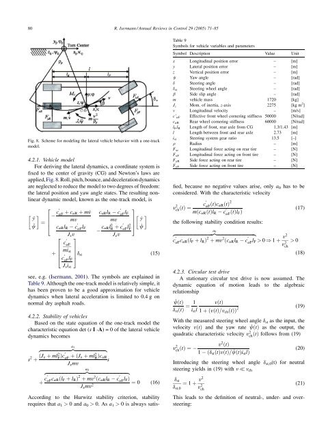
Fig. 8. Scheme for modeling the lateral vehicle behavior with a one-track
model.
4.2.1. Vehicle model
For deriving the lateral dynamics, a coordinate system is
fixed to the center of gravity (CG) and Newton’s lawsare
applied, Fig. 8. Roll, pitch, bounce, and deceleration dynamics
are neglected to reduce the model to two degrees of freedom:
the lateral position and yaw angle states. The resulting nonlinear
dynamic model, known as the one-track model, is
2
¨y
¨c ¼
6
4
c 0
aF þ caR þ m˙v
mv
6
þ 6
4
caRlR c 0
aF lF
2
Jzv
3
7
c 0
aF
mist
c 0
aFlF 5 dst
Jsist
caRlR c 0
aF lF
caRl 2 R
mv
þ c0
Jzv
aF l2 F
3
7
5
˙y
˙c
(15)
see, e.g. (Isermann, 2001). The symbols are explained in
Table 9. Although the one-track model is relatively simple, it
has been proven to be a good approximation for vehicle
dynamics when lateral acceleration is limited to 0.4 g on
normal dry asphalt roads.
4.2.2. Stability of vehicles
Based on the state equation of the one-track model the
characteristic equation det (s I -A) = 0 of the lateral vehicle
dynamics becomes
a1
zfflfflfflfflfflfflfflfflfflfflfflfflfflfflfflfflfflfflfflfflfflfflfflfflfflffl}|fflfflfflfflfflfflfflfflfflfflfflfflfflfflfflfflfflfflfflfflfflfflfflfflfflffl{
s 2 þ ðJz þ ml2 FÞc0aF þðJz þ ml2 RÞcaR s
Jzmv
þ c0aF
caRðlF þ lRÞ 2 þ mv2ðcaRlR c 0
aFlFÞ Jzmv2 a0
zfflfflfflfflfflfflfflfflfflfflfflfflfflfflfflfflfflfflfflfflfflfflfflfflfflfflfflfflfflfflfflfflffl}|fflfflfflfflfflfflfflfflfflfflfflfflfflfflfflfflfflfflfflfflfflfflfflfflfflfflfflfflfflfflfflfflffl{
¼ 0 (16)
According to the Hurwitz stability criterion, stability
requires that a1 > 0 and a0 > 0. As a1 > 0 is always satis-
R. Isermann / Annual Reviews in Control 29 (2005) 71–85
Table 9
Symbols for vehicle variables and parameters
Symbol Description Value Unit
x Longitudinal position error – [m]
y Lateral position error – [m]
z Vertical position error – [m]
c Yaw angle – [rad]
d Steering angle – [rad]
dst Steering wheel angle – [rad]
b Side slip angle – [rad]
m vehicle mass 1720 [kg]
Jz Mom. of inertia, z-axis 2275 [kg m 2 ]
v Longitudinal velocity – [m/s]
c’aF Effective front wheel cornering stiffness 50000 [N/rad]
caR Rear wheel cornering stiffness 60000 [N/rad]
lF,lR Length of front, rear axle from CG 1.3/1.43 [m]
l Length between front and rear axle 2.73 [m]
ist Steering system gear ratio 13.5 [–]
r Radius – [m]
Fxr Longitudinal force acting on rear tire – [N]
FxF Longitudinal force acting on front tire – [N]
FyR Side force acting on rear tire – [N]
FyF Side force acting on front tire – [N]
fied, because no negative values arise, only a0 has to be
considered. With the characteristic velocity
v 2 c
chðtÞ ¼
0
2
aFðtÞcaRðtÞ mðcaRðtÞlR c 0
aFðtÞlFÞ (17)
the following stability condition results:
a0
zfflfflfflfflfflfflfflfflfflfflfflfflfflfflfflfflfflfflfflfflfflfflfflfflfflfflfflfflfflfflfflffl}|fflfflfflfflfflfflfflfflfflfflfflfflfflfflfflfflfflfflfflfflfflfflfflfflfflfflfflfflfflfflfflffl{
c 0
aF caRðlF þ lRÞ 2 þ mv 2 ðcaRlR c 0
aF lF
> 0 ) 1 þ v2
v2 > 0
ch
(18)
4.2.3. Circular test drive
A stationary circular test drive is now assumed. The
dynamic equation of motion leads to the algebraic
relationship
˙cðtÞ 1 vðtÞ
¼
dstðtÞ istl 1 þðvðtÞ=vchðtÞÞ 2
(19)
With the measured steering wheel angle dst as the input, the
velocity vðtÞ and the yaw rate ˙cðtÞ as the output, the
quadratic characteristic velocity v2 chðtÞ follows from (19)
v 2 chðtÞ ¼
v 2 ðtÞ
1 ðdstðtÞvðtÞ= ˙cðtÞistlÞ
(20)
Introducing the steering wheel angle dst,0(t) for neutral
steering yields in (19) with n nch
dst
dst;0
¼ 1 þ v2
v 2 ch
(21)
This leads to the definition of neutral-, under- and oversteering: