Model-based fault-detection and diagnosis ... - web page for staff
Model-based fault-detection and diagnosis ... - web page for staff
Model-based fault-detection and diagnosis ... - web page for staff

You also want an ePaper? Increase the reach of your titles
YUMPU automatically turns print PDFs into web optimized ePapers that Google loves.
72<br />
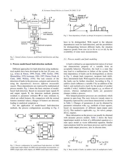
Fig. 1. General scheme of process model-<strong>based</strong> <strong>fault</strong>-<strong>detection</strong> <strong>and</strong> <strong>diagnosis</strong>.<br />
2. Process model-<strong>based</strong> <strong>fault</strong>-<strong>detection</strong> methods<br />
Different approaches <strong>for</strong> <strong>fault</strong>-<strong>detection</strong> using mathematical<br />
models have been developed in the last 20 years, see,<br />
e.g., (Chen & Patton, 1999; Frank, 1990; Gertler, 1998;<br />
Himmelblau, 1978; Isermann, 1984, 1997; Patton, Frank, &<br />
Clark, 2000; Willsky, 1976). The task consists of the<br />
<strong>detection</strong> of <strong>fault</strong>s in the processes, actuators <strong>and</strong> sensors by<br />
using the dependencies between different measurable<br />
signals. These dependencies are expressed by mathematical<br />
process models. Fig. 1 shows the basic structure of model<strong>based</strong><br />
<strong>fault</strong>-<strong>detection</strong>. Based on measured input signals U<br />
<strong>and</strong> output signals Y, the <strong>detection</strong> methods generate<br />
residuals r, parameter estimates ˆ Q or state estimates ˆx,<br />
which are called features. By comparison with the normal<br />
features (nominal values), changes of features are detected,<br />
leading to analytical symptoms s.<br />
For the application of model-<strong>based</strong> <strong>fault</strong>-<strong>detection</strong><br />
methods, the process configurations according to Fig. 2<br />
Fig. 2. Process configuration <strong>for</strong> model-<strong>based</strong> <strong>fault</strong>-<strong>detection</strong>: (a) SISO<br />
(single-input single-output); (b) SISO with intermediate measurements; (c)<br />
SIMO (single-input multi-output); (d) MIMO (multi-input multi-output).<br />
R. Isermann / Annual Reviews in Control 29 (2005) 71–85<br />
Fig. 3. Time-dependency of <strong>fault</strong>s: (a) abrupt; (b) incipient; (c) intermittent.<br />
have to be distinguished. With regard to the inherent<br />
dependencies used <strong>for</strong> <strong>fault</strong>-<strong>detection</strong>, <strong>and</strong> the possibilities<br />
<strong>for</strong> distinguishing between different <strong>fault</strong>s, the situation<br />
improves greatly from case (a) to (b) or (c) or (d), by the<br />
availability of some more measurements.<br />
2.1. Process models <strong>and</strong> <strong>fault</strong> modeling<br />
A <strong>fault</strong> is defined as an unpermitted deviation of at least<br />
one characteristic property of a variable from an<br />
acceptable behavior. There<strong>for</strong>e, the <strong>fault</strong> is a state that<br />
may lead to a malfunction or failure of the system. The<br />
time dependency of <strong>fault</strong>s can be distinguished, as shown<br />
in Fig. 3, abrupt <strong>fault</strong> (stepwise), incipient <strong>fault</strong> (driftlike),<br />
intermittent <strong>fault</strong>. With regard to the process models,<br />
the <strong>fault</strong>s can be further classified. According to Fig. 4<br />
additive <strong>fault</strong>s influence a variable Y by an addition of the<br />
<strong>fault</strong> f, <strong>and</strong>multiplicative <strong>fault</strong>s by the product of another<br />
variable U with f. Additive <strong>fault</strong>s appear, e.g., as offsets of<br />
sensors, whereas multiplicative <strong>fault</strong>s are parameter<br />
changes within a process.<br />
Now lumped-parameter processes are considered, which<br />
operate in open loop. The static behavior (steady states) is<br />
frequently expressed by a non-linear characteristic as shown<br />
in Table 1. Changes of parameters bi can be obtained by<br />
parameter estimation with, e.g., methods of least squares,<br />
<strong>based</strong> on measurements of different input–output pairs<br />
[Y j,U j]. This method is applicable, e.g., <strong>for</strong> valves, pumps,<br />
drives, engines.<br />
More in<strong>for</strong>mation on the process can usually be obtained<br />
with dynamic process models. Table 2 shows the basic<br />
input/output models in <strong>for</strong>m of a differential equation or a<br />
state space model as vector differential equation. Similar<br />
representations hold <strong>for</strong> non-linear processes <strong>and</strong> <strong>for</strong> multiinput<br />
multi-output processes, also in discrete-time.<br />
Fig. 4. Basic models of <strong>fault</strong>s: (a) additive <strong>fault</strong>; (b) multiplicative <strong>fault</strong>s.